Rock Physics Based Interpretation of Seismically Derived Elastic Volumes

Introduction

Most rock physics models are designed to arrive at the elastic properties of porous rocks from their petrophysical properties, such as the total porosity, mineralogy, organic matter content in unconventional reservoirs, and pore fluid saturation and individual fluid phase properties. Such current models are based on various effective medium theories taking into account the pore-space geometry, degree of cementation, as well as such conditions as the differential pressure and water saturation. These models (or transforms) usually predict the elastic P- and S-wave impedances (I_p and I_s, respectively), as well as the bulk density (ρ_b), from the aforementioned petrophysical and environmental inputs. These transforms are often used in the forward-modeling mode to generate the elastic properties and the resulting synthetic seismograms for geologically plausible what-if scenarios for varying inputs, among them porosity, lithology, and saturation. Can these models be used in an inverse mode to generate the seismic-scale petrophysical variables from seismically derived impedances and density?

The seemingly unresolvable issue of such interpretation is the so-called “rock physics bottleneck,” meaning that the few elastic properties depend on a larger number of volumetric and environmental inputs, such as porosity, mineralogy, water saturation, differential stress, and rock-frame texture (e.g., cemented vs. friable sediments). Hence, the interpretation is impossible in a strictly mathematical sense. Yet, by carefully analyzing controlled-experiment data, especially those from wireline measurements, and putting this analysis into the geological context, one can resolve even a single elastic input for more than one volumetric variable. For example, Dvorkin and Alkhater (2004) found, by plotting I_p vs. porosity (ϕ) from wireline data in an unconsolidated-sand offshore reservoir, that two very distinct I_p–ϕ trends emerge, one for the gas and the other for the liquid (oil and water) leg. This finding helped obtain volumes of the pore fluid and porosity from only one variable, the seismically derived acoustic impedance.

This concept of adding a site-specific equation to the rock physics model was further developed by Arevalo-Lopez and Dvorkin (2016) and Arevalo-Lopez and Dvorkin (2017) where simultaneous impedance inversion was performed to quantify porosity, mineralogy, and pore fluid in a siliciclastic turbidite oil reservoir offshore northwest Australia. Specifically, the I_p/I_s ratio was utilized as a hydrocarbon identifier for oil-saturated rock where this ratio was small. Once the pore fluid was thus identified, a theoretical rock physics model was used to estimate the porosity and clay content from the two inputs, I_p and I_s, in a binary-mineral environment, a quartz/clay system.

Of course, the high-quality simultaneous impedance inversion results can be interpreted in a strictly mathematical fashion. Wollner et al. (2017) used all three seismic-scale variables, I_p, I_s, and ρ_b, to arrive at the total porosity, clay content, and water saturation. The main contribution of that work was to translate the well-scale rock physics model into the seismic scale. Specifically, it was found that unlike at the wellbore scale, the relation between the effective bulk modulus of the gas/brine system and S_w at the seismic scale was according to the “patchy” rather than “uniform” saturation scheme.

Here we revisit this interpretation concept and give two examples thereof where a mathematical rock physics model was supplemented with a geology-based pore-fluid discrimination thus allowing for quantifying the porosity, mineralogy, and the pore fluid from only one (I_p) or two (I_p and I_s) inputs.

As mentioned above, there are at least two issues to be addressed during such interpretation. One is the issue of the spatial scale. Indeed, a rock physics model is usually derived from the laboratory or wireline data where the spatial resolution is on the order of a ft. The question is whether these transforms are usable at the seismic scale of tens or hundreds of ft. The other issue is related to the fact that the number of petrophysical inputs is often larger than just the two (I_p and I_s) and at the most three (I_p, I_s, and ρ_b) variables provided by the simultaneous impedance inversion. How can two (or three) equations be resolved for more than two (or three) unknowns?

To test the concept, we first employed the arguably simplest rock physics model, the Raymer et al. (1980) transform that relates V_p to porosity, pore fluid properties, and mineralogy. We assumed a binary quartz/clay mineralogy and fixed fluid properties. By creating an objective function that minimizes the difference between the measured and assumed I_p and I_s as a function of porosity and clay content, we successfully interpreted these two elastic variables for the petrophysical variables in question.

Next, we used wireline data from an offshore oil chalk reservoir to, once again, interpret the measured impedances for the desired petrophysical properties, porosity and water saturation. In this formation, there is a fairly robust relation between the porosity and water saturation. Specifically, due to diagenetic processes, the high-porosity rock contains oil, while the low-porosity rock is essentially 100% water saturated. Prior to interpretation, we established that the velocity-porosity model for this formation is the stiff-rock model (the modified upper Hashin-Shtrikman bound). By using this model in reverse within the objective function, as well as the abovementioned relation between porosity and the pore fluid, we accurately predicted the porosity and saturation from I_p and I_s both at the well and also using the spatially upscaled impedances to address this interpretation method at the seismic scale.

In the second case study, we used wireline data from an onshore clastic reservoir with oil. We had to interpret I_p and I_s for three variables, the total porosity, clay content, and water saturation. As in the first case study, the rock physics diagnostics indicated that the velocity-porosity model was the stiff-rock model, now applied to the quartz/clay mineralogy. The additional equation required to resolve the two elastic inputs for the three unknowns was very similar to that used in the first case study. It appeared that although the two oil fields under examination are located thousands of miles apart and in very different depositional environments, the diagenetically-driven relations between the porosity and pore fluid are qualitatively the same. The low-porosity intervals were predominantly water-saturated, while the higher-porosity intervals contained oil. By using the respective porosity-saturation threshold, we accurately interpreted the measured impedances for the desired three variables at the well and also at the seismic scale using mathematically upscaled elastic and volumetric properties.

The new methods and examples introduced here show how to combine mathematical rock physics models with geology-driven quantitative relations to interpret seismically-derived impedance volumes for volumetric reservoir attributes.

Proof of Concept

Arguably, the simplest rock physics model is the Raymer et al. (1980) transform relating the mineralogy and pore-fluid properties to V_p and V_s as:

$\begin{array}{l}{V}_p=V_{ps}{\left(1-\varphi \right)}^2+V_{pf}\varphi ;\\ V_s=V_{ss}{\left(1-\varphi \right)}^2\sqrt{\left(1-\varphi \right){\rho }_s/{\rho }_b}\end{array}(1)$

where V_ps and V_ss are the P- and S-wave velocities in the mineral matrix, respectively; V_pf is the P-wave velocity in the pore fluid; ϕ is the total porosity; and ρ_s and ρ_b are the density of the mineral matrix and the bulk density, respectively. The second line in Eq. 1 is due to Dvorkin (2008). The P- and S-wave impedances (I_p and I_s) are simply

$I_p={\rho }_b{V}_p;I_s={\rho }_b{V}_s,(2)$

Assume for simplicity that the mineralogy is binary (quartz/clay). The densities of quartz and clay are both assumed 2.65 g/cc. The bulk moduli of quartz and clay are 36.6 and 21 GPa, respectively, while their shear moduli are 45 and 7 GPa, respectively. Let us next generate three forward modeling scenarios for varying porosity, clay content (C), and water saturation (S_w). The inputs to these three scenarios are listed in Table 1. Also, assume that the immiscible pore-fluid phases are gas and brine whose densities are 1.05 and 0.24 g/cc, respectively, while their bulk moduli are 3.09 and 0.11 GPa, respectively.

TABLE 1

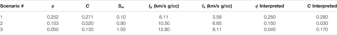
TABLE 1. Inputs (porosity ϕ, clay content C, and water saturation S_w) for forward modeling scenarios using the Raymer et al. (1980) model and the computed P- and S-wave impedances (I_p and I_s, respectively).

Because the P- and S-wave impedance volumes are usually the product of simultaneous impedance inversion, our goal is to arrive at the volumetric inputs listed in Table 1 using these impedances. Specifically, first we forward-model these impedances I_p and I_s using Eqs. 1, 2 and the inputs from the aforementioned three scenarios. These forward modeling results are also listed in Table 1.

Our next goal is to arrive at these volumetric inputs now using these I_p and I_s as inputs and, once again, Eqs. 1, 2. Needless to say that we cannot derive more than two unknowns from two inputs. Hence, we select these two unknowns as ϕ and C and assume that S_w and the resulting bulk modulus and density of the pore fluid are known. Next we cycle through a matrix of as yet unknown ϕ and C and generate an objective function

$F_o={\left(I_p-I_{p0}\right)}^2+{\left(I_s-I_{s0}\right)}^2,(3)$

where I_p0 and I_s0 are now the known input impedances from forward modeling (Table 1).

We find the minimum of this function and select ϕ and C associated with this minimum as our interpretation results. We have found that in this example, the objective function has only one global minimum (Figure 1) thus rendering interpretation unique. Earlier studies (Arevalo-Lopez and Dvorkin, 2016, 2017; and; Wollner et al., 2017) also point at uniqueness of such interpretation. This is also the case in the following two case studies.

FIGURE 1

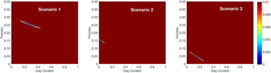
FIGURE 1. The objective function as given by Eq. 3 plotted inside the porosity (vertical axis) and clay content (horizontal axis) mesh with the minima shown in color (blue) on the solid-color background.

These interpretation results for the aforementioned three scenarios are also listed in Table 1. As we can see, they are very close to the volumetric inputs. The small mismatch is caused by the coarseness of the lookup table for the variable I_p and I_s. A much more accurate match can be attained if the search grid in this table is fine enough.

The location of the minimum of the objective function for these three scenarios is shown in Figure 1, which illustrates that using the two impedances as an input for interpretation produces distinctive extrema.

Case Study A: Carbonate Oil Field

Porosity and hydrocarbon saturation are two important parameters for resource assessment. In this case study, we investigate the applicability of our rock physics based seismic interpretation workflow to quantifying porosity and pore fluid from measured elastic properties. Wireline data of two wells within oil-bearing off-shore chalk deposits with high-to-medium porosity were used in this exercise. The mineralogy is practically 100% calcite. The goal is to interpret the elastic impedances for the desired petrophysical properties, namely porosity and water saturation. The rock physics analysis of the wireline data used here is given by Dvorkin and Alabbad (2019). Here we use these data to illustrate our interpretation strategy.

Sensitivity to Pore Fluid. Traditional approach to discriminating the pore fluid from seismic data is based on the difference in the AVO response at the reservoir depending on whether the reservoir contains water or hydrocarbon. This difference is, in turn, governed by the V_p/V_s ratio (or Poisson’s ratio) that is low in gas-saturated rock and relatively high in 100% wet rock. This difference affects the slope of the AVO curve, also known as the gradient.

However, in some cases, the effect of the pore fluid on the elastic properties is weak. This may happen where the difference between the compressibility and density of the hydrocarbon and brine is small (as in oil vs. water case) and/or where the rock frame is stiff, even at high porosity (as in some carbonates). An example of such a situation is shown in Figure 2 based on the laboratory measurements of V_p and V_s in dry rock vs. hydrostatic confining stress. These measurements were carried out on several samples extracted from the wells under examination. As stated earlier, the mineralogy is essentially 100% calcite.

FIGURE 2

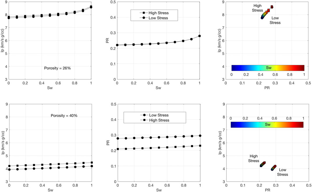
FIGURE 2. I_p (left) and ν (center) vs. S_w as computed from the dry-rock data using fluid substitution. Circles are for the low-stress data, while squares are for the high-stress data. Top: Sample with porosity 26%. Bottom: Sample with porosity 40%. The third frame in each row shows I_p vs. ν cross-plots color-coded by S_w.

We selected two samples, one with porosity (ϕ) 26% and the other with porosity 40%. Fluid substitution was conducted using Gassmann’s (1951) equation assuming the bulk modulus of the mineral phase 62.44 GPa, the average between the two values for pure calcite as described in Dvorkin and Alabbad (2019) and listed in Table 2. The properties of the brine and oil are also listed in Table 2. The bulk modulus of the pore fluid for S_w varying between zero and 100% was computed as the harmonic average of those of brine and oil, while the density was computed as the arithmetic average of the respective densities. The velocity measurements were conducted in the hydrostatic confining stress range between 7 and 40 MPa. For this example, we selected the data obtained at the lowest and highest stresses.

TABLE 2

TABLE 2. The elastic moduli and densities of the rock components.

The results for the sensitivity of I_p and Poisson’s ratio (v) to S_w are shown in Figure 2. As we can see, this sensitivity is very weak, no matter whether the sample has high or low porosity.

Fluid substitution performed on wireline data from the same field (Figure 3) also shows very weak sensitivity of the elastic properties to water saturation (Dvorkin and Alabbad, 2019) even in the intervals with relatively high porosity. This conclusion is reconfirmed by the cross-plots also shown in Figure 3. Indeed, even at the highest porosity, the difference between the in-situ I_p and that computed for 100% water saturation is significantly smaller than the vertical variations of this variable, which will make it difficult to elucidate the pore-fluid effect in seismic data. The respective variations in Poisson’s ratio are also relatively small.

FIGURE 3

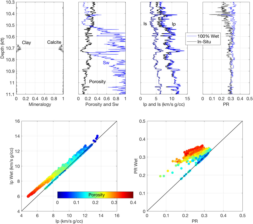
FIGURE 3. Top: Depth plots for one of the wells from the field under examination. From left to right: Mineralogy; the total porosity and water saturation; P- and S-wave impedances; and Poisson’s ratio. In the last two frames, black curves are for measured properties, while blue curves are for these properties at 100% water saturation computed using Gassmann’s (1951) fluid substitution. Bottom: Cross-plots of the in-situ vs. 100% wet P-wave impedance (left) and Poisson’s ratio (right) color-coded by the total porosity and using the data shown in top row.

Pore Fluid Discrimination. The above plots indicate low sensitivity of both the impedance and Poisson’s ratio to the pore fluid. Does this mean that in this situation we cannot interpret seismically derived impedances for pore fluid? Yes, if we solely rely on mathematical fluid substitution as the primary means of pore fluid identification. No, if we look deeper into interrelations among various rock attributes.

By plotting the impedance vs. porosity (Figure 4), we observe that in this case, the low-porosity intervals contain practically 100% water, while high-porosity intervals contain sizable volumes of oil. Respectively, rock with oil has relatively low impedance, while rock with water has higher impedance. It appears that the porosity determines the pore fluid. In fact, the effect is the opposite: the pore fluid has influenced the porosity evolution. Where oil entered the porous chalk, the diagenesis was halted. At the same time, where brine remained dominant, diagenesis and porosity reduction continued (Dvorkin and Alabbad, 2019).

FIGURE 4

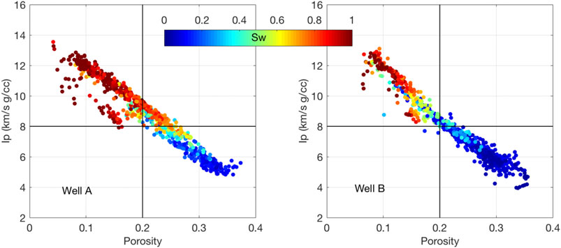
FIGURE 4. Cross-plots of I_p as measured vs. porosity color-coded by water saturation for Wells A and B.

Based on Figure 4, we can propose now that the rock contains oil where the total porosity exceeds approximately 20% and it is 100% wet in the lower-porosity intervals. The respective I_p cutoff is about 8 km/s g/cc.

Rock Physics Modeling.Dvorkin and Alabbad (2019) show that the stiff-sand model (e.g., Dvorkin et al., 2014) accurately describes the wireline data in the carbonate oil field under examination. This model has the mathematical form of the modified upper Hashin-Shtrikman bound. The inputs specific to this case study are: 30 MPa differential pressure; 0.40 critical porosity; and 6 coordination number. The fairly tight impedance-porosity cross-plots (Figure 4) were accurately bounded by this model curves using two different pure-calcite end-member properties as listed in Table 2.

Figure 5 compares the model-based computed elastic properties to those measured in situ. The former were computed using the following inputs: mineralogy (calcite and clay); the total porosity; and water saturation. The effective elastic moduli of the mineral matrix were obtained as Hill’s (1952) average of those of calcite and clay, while its density was the arithmetic average of the respective densities. The densities and bulk moduli of the two fluid phases, oil and brine, were computed from pore pressure, temperature, salinity, oil API gravity, and gas-to-oil ratio using Batzle and Wang (1992) equations. The effective bulk modulus of the immiscible oil/brine system was the harmonic average of the components, while the density was the arithmetic average. All these inputs are listed in Table 2.

FIGURE 5

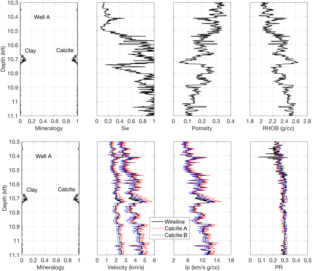
FIGURE 5. Wireline curves at in-situ conditions for Well A (top) with the stiff-sand model curves (bottom) shown in the velocity, impedance, and Poisson’s ratio frames using the Calcite A (red) and Calcite B (blue) inputs.

The modeled elastic property curves using the Calcite A and B inputs tightly bound the wireline data at in-situ conditions for both wells under examination. An example for Well A is shown in Figure 5.

Interpretation at Well A.Figure 3 indicates that the sensitivity of the elastic properties to the pore fluid (or water saturation) is weak. At the same time, both the P- and S-wave impedances show a strong dependence on porosity. Hence, our interpretation strategy in this case study is to interpret the impedances for the total porosity and then use the porosity-saturation cutoff shown in Figure 4 to predict the pore fluid.

With this goal in mind, let us explore the sensitivity of porosity interpretation to the assumed pore fluid and the elastic properties of the calcite (Calcite A vs. B). Specifically, we use the same interpretation method as described in the previous section and conduct it along the well at each depth station. We examine four variants: 1) S_w = 0.20 and Calcite A; 2) S_w = 1.00 and Calcite A; 3) S_w = 0.20 and Calcite B; and 4) S_w = 1.00 and Calcite B. Also, we implement this interpretation workflow based only on the measured I_p, as well as based on both I_p and I_s. The interpretation results shown in Figure 6 indicate that the interpreted porosity only weakly depends on these variants.

FIGURE 6

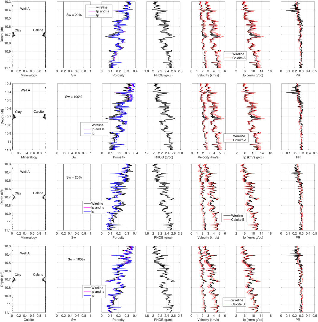
FIGURE 6. Interpretation for porosity using the four variants as described in the text and also using only I_p and I_p and I_s together. From top to bottom: Variants 1, 2, 3, and 4. The interpreted porosity curves are shown in color and described in the legends. Red curves in the elastic property frames are from the stiff-sand model using the respective inputs.

Based on the observed weak sensitivity of porosity interpretation to the model inputs, we will simply use single values for the bulk and shear moduli of pure calcite as the means of the respective moduli of Calcite A and B. Namely, these bulk and shear moduli are 66.44 and 25.38 GPa, respectively.

Seismic-Scale Interpretation. In order to show how our interpretation method works at the seismic scale, we first use the Backus (1962) averaging to upscale the elastic curves in both wells. The example using Well A is shown in Figure 7, where we also show the arithmetically upscaled porosity, bulk density, and water saturation curves.

FIGURE 7

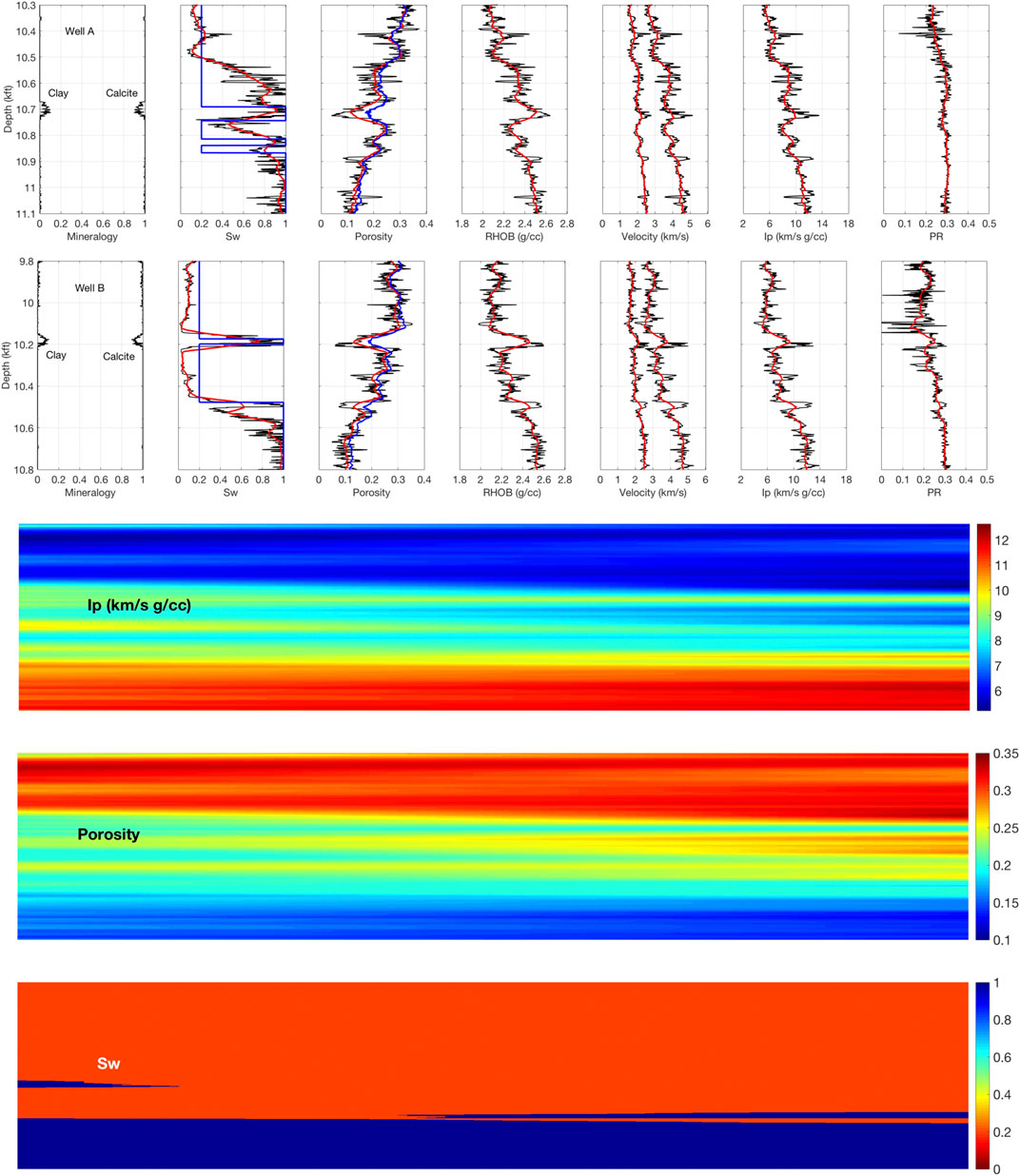
FIGURE 7. Top two rows: Upscaled curves in Well A and B (red) and interpretation for porosity and water saturation (blue). Bottom three rows: I_p pseudo-section (top) and the interpreted porosity (middle) and water saturation (bottom) sections between Well A (left) and B (right).

This upscaling is conducted using a running window of approximately 1/8 of the wavelength (about 50 ft or 15 m) assuming 40 Hz frequency. During interpretation, we had to assign the effective bulk modulus and density of the brine/oil system. To do this, we used the cutoffs shown in Figure 4 by assuming S_w = 1.00 for porosity smaller 0.20 and S_w = 0.20 for porosity greater than or equal 0.20.

The interpreted porosity and water saturation curves for both wells are shown in Figure 7. The interpreted porosity closely follows the upscaled porosity curves in both wells. The interpreted S_w appears blocky simply because of the porosity-saturation cutoff we have chosen. This interpretation clearly identifies oil-saturated zones in Well B. At the same time, it appears overly optimistic in Well A, where it shows high oil saturation in the lower part of the reservoir. Of course, we could have had a more precise reservoir delineation in this well if we have chosen a different porosity cutoff. This may be a strategy for providing upper and lower reserve estimates during field interpretation. Here, for the purpose of simplicity, we will use the originally selected cutoff.

In order to illustrate the application of our methodology to an impedance inversion section, we generate a pseudo-section for the upscaled I_p between Well A and the upper portion of Well B (Figure 7, bottom) using linear interpolation along the offset. These pseudo-seismic sections were produced using the Backus-upscaled P- and S-wave impedances from the two wells. First, we matched the lengths of the data vectors from both wells by simple linear interpolation. Then, a 2D linear interpolation was performed on a monotonic and plaid matrix with the length of the well along the Y-axis (depth or time) and the distance between the two wells along the X-axis (offset). In this example, the distance between the wells was assigned to be 100 pixels.

The resulting 2D P- and S-wave impedances are then used as an input to the seismic interpretation workflow. Let us emphasize that these are not real seismic sections but rather pseudo-sections generated for purely visual purpose to show how the proposed interpretation might look in a real seismic world.

Next, we apply the same interpretation routine as used to generate the porosity and S_w profiles. As before, we only use I_p as the input, as well as the average calcite elastic moduli and density. The results shown in Figure 7 (last two rows) indicate that indeed our interpretation method provides reasonable porosity and water saturation estimates.

Case Study B: Clastic Oil Field

The oil-bearing clastic reservoir under examination is composed of predominantly quartz low-to-medium porosity rock. The mineralogy is binary, quartz/clay. The oil has low gas-to-oil ratio and fairly low (about 20) API gravity. The rock physics diagnostics of wireline data from this field was conducted by Dvorkin (2019). The elastic moduli and densities of the minerals and fluid phases used are listed in Table 3.

TABLE 3

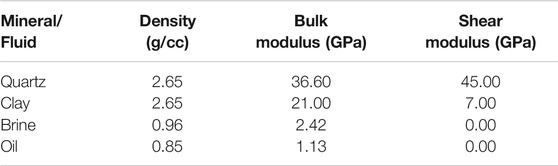
TABLE 3. Densities and elastic moduli of the minerals and pore-fluid phases used in rock physics modeling.

In the present case study, we will use two wells out of four described in Dvorkin (2019). The respective wireline data are shown in Figure 8.

FIGURE 8

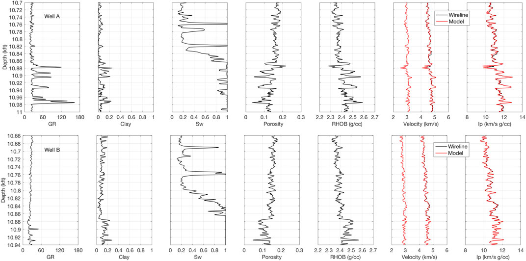
FIGURE 8. Wireline data for Well A (top) and Well B (bottom). From left to right: GR; clay content; water saturation; the total porosity; bulk density; V_p and V_s; and the P-wave impedance. Black curves are for measured properties, while red curves are for model-predicted.

Only the P-wave velocity data were available in this study. The rock physics model determined based on these data (Dvorkin, 2019) is the stiff-rock model (the modified upper Hashin-Shtrikman bound), similar to the model used in the first case study. The model parameters are as follows: the differential pressure 50 MPa; coordination number 12; and critical porosity 0.40.

The total porosity was computed from the measured bulk density, water saturation, and mineralogy using the mass-balance equation. The clay content was model-predicted from the measured V_p and the total porosity using the stiff-rock model in reverse as described in Dvorkin et al. (2014). Finally, V_s was predicted from the mineralogy, porosity, and pore fluid, once again, using the same rock physics model.

Next, we assume that the measured V_p, bulk density, and predicted V_s are the inputs to the interpretation workflow, compute the respective I_p and I_s, and interpret these elastic properties for the total porosity, clay content, and water saturation. As in the previous case study, we only have two inputs (I_p and I_s) and require three outputs.

The missing equation is very similar to that used in the first case study. Dvorkin (2019) shows that in this clastic reservoir we face diagenesis-driven pore fluid discrimination. Namely, the intervals with oil have porosity higher that approximately 15%, while the 100%-wet intervals have porosity below 15%. We utilize this finding by assuming that S_w = 0.20 for ϕ > 0.15 and S_w = 1.00 for smaller porosity. The ensuing interpretation results at both wells are shown in Figure 9. We observe accurate match between the measured and interpreted variables.

FIGURE 9

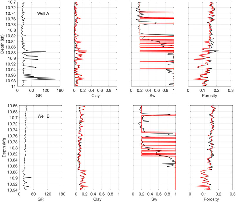
FIGURE 9. Interpretation results (red) for Well A (top) and Well B (bottom). The measured variables are shown in black.

Next, after validating the interpretation workflow at the wireline scale, we test it at the seismic scale by applying it to the Backus-upscaled elastic properties, same as described in the previous case study. Once again, the interpretation results accurately match the arithmetically-upscaled porosity, clay content, and water saturation, except for minor S_w misinterpretation intervals (Figure 10). Finally, to illustrate the application of our interpretation method to a seismic section, we generate a pseudo-section of I_p and I_s between the two wells with the interpretation results also shown in Figure 10.

FIGURE 10

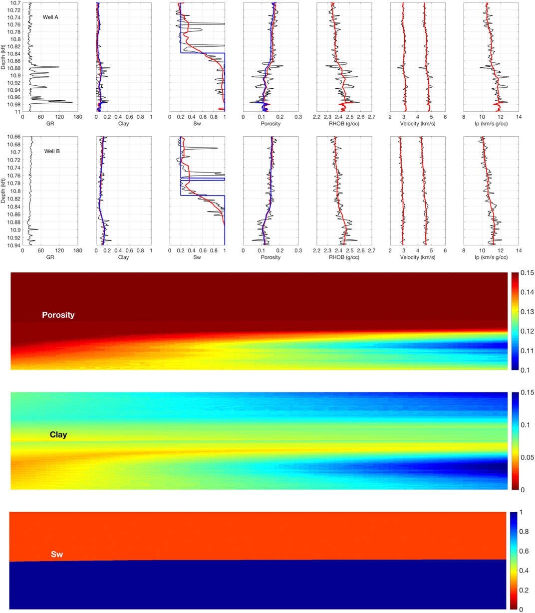
FIGURE 10. Top: Interpretation results at the seismic scale (blue) for Well A and B. The upscaled variables are shown in red, while the wireline-scale variables are shown in black. Bottom: Interpreted porosity (top), clay content (middle), and water saturation (bottom) sections between Well B (left) and A (right). The inputs used were the interpolated upscaled I_p and I_s.

Discussion

The field of impedance inversion is very extensive and extremely mathematically involved (e.g., Russell, 1999; Mallick, 2001; Mallick, 2007; and; Lau et al., 2002). The challenge here is to derive absolute elastic properties from seismic waveforms that depend on the relative elastic property contrast in the subsurface. Still, even where accurate impedance volumes are produced, they hardly provide the information needed for exploration and development. Arguably, the ultimate product of such inversion should be an interpretation for porosity, saturation, and lithology.

This is why such interpretation is now considered one of the new frontiers in exploration. Previous attempts include the already quoted work by Arevalo-Lopez and Dvorkin (2016) and Arevalo-Lopez and Dvorkin (2017) and Wollner et al. (2017). Souvannavong et al. (2013) present a petro-elastic concept of such inversion for an offshore carbonate field.

Here we revisit the concept of deterministic rock-physics based interpretation of seismically-derived elastic properties and show how geology-based information can be incorporated into this workflow. The two new case studies presented here illustrate this concept. The novelty is the combination of the rock physics diagnostics methodology, spatial upscaling of the ensuing rock physics transforms, and geology-based fluid-porosity-impedance discrimination. Finding such relationships between different rock petrophysical properties is key to extracting rock properties from its impedance response. Essential also is the optimization method using an objective function. This workflow chart is shown in Figure A1.

In both cases, the theoretical stiff-rock model (the modified upper Hashin-Shtrikman bound) appears to accurately quantify the data. This model, as any other rock physics model, requires a number of assumptions, including the elastic properties of the mineral components. In the case studies under examination, these inputs were assigned commonly-used and well documented values.

Another important assumption is the absence of velocity-frequency dependence in the wireline and seismic frequency ranges. Such dependence (dispersion) is well documented when comparing laboratory data acquired at about 1 MHz frequency with low-frequency measurements (see, e.g., Mavko et al., 2020). It also becomes apparent when comparing ultrasonic velocity measurements of liquid-saturated porous materials with the results of Gassmann’s (1951) fluid substitution on the same dry samples. Such dispersion can occur even at wireline and seismic frequencies where the pore fluid has very high viscosity, such as heavy oil. In the cases we examine here, the pore fluid components are water and conventional oil. This is why we feel it is reasonable to neglect velocity-frequency dependence and use the low-frequency fluid substitution methods.

Such fluid substitution as employed here assumes that the effective bulk modulus of the brine/hydrocarbon system is the harmonic average of the elemental bulk moduli. In other words, we use the concept of “uniform” fluid distribution in the pore space as opposed to “patchy” distribution. The latter may occur during oil recovery due to uneven displacement of the fluid phases in real time (e.g., Dvorkin and Nur, 1998; Monachesi et al., 2020). However, it is reasonable to assume that in exploration studies, under the condition of geologically long-term fluid equilibrium, fluid distribution is uniform (e.g., Arevalo-Lopez and Dvorkin, 2017).

An important development introduced here is the application of the rock physics models at the seismic scale required in order to ensure that the interpretation workflow proposed can be used with real seismic data. To facilitate this application, we generated synthetic seismic-scale impedance inversion data for the P- and S-wave impedances by using the standard Backus (1962) elastic upscaling. The upscaling running window was selected as appropriate for the seismic frequency range. Such upscaling was conducted at each well and then synthetic impedance sections were generated by simple deterministic interpolation between the wells. Because here to prove the concept we deal with synthetic seismic data, no uncertainty needs to be taken into consideration.

At the same time, impedance inversion of real seismic data often carries a significant element of uncertainty as it requires adjusting many inversion parameters and, as a result, is often subjective (e.g., Russell, 1999; Mallick, 2007). The best way of reducing this uncertainty is to ensure an accurate match of the seismically-derived impedances and density at the wells. The interpretation method offered here carries additional controls on inversion uncertainty as it translates the elastic properties into porosity, mineralogy, and water saturation, the quantities whose reasonableness can be ascertained from the geological and sedimentological viewpoint.

There are several factors that contribute to the efficiency and accuracy of this workflow. First, it is building a robust rock physics model that captures the relationship between rock’s elastic and volumetric properties. Second, it is the sensitivity of the model to small changes in the volumetric variables. It is desirable to have a finer mesh, however, it comes with a computational cost which also needs to be accounted for.

Finally, the physics-based deterministic approach discussed here opens ways for a data-driven stochastic analysis and probabilistic interpretation.

Conclusion

The deterministic seismic interpretation method presented here depends on combining mathematical rock physics models with a site-specific geology-based pore-fluid discrimination to quantifying the total porosity, mineralogy, and the pore fluid from one (I_p) or two (I_p and I_s) inputs. The pore fluid in these two case studies played a role in the evolution of porosity, which helped supplement the mathematical rock physics models with an additional geology-driven equation and, by so doing, enhance the interpretation ability. This method is applicable at the seismic-scale where the impedance is less sensitive to fine-scale changes in the reservoir.

Data Availability Statement

The datasets presented in this article are not readily available due to data confidentiality. Requests to access the datasets should be directed to jackdvorkin007@gmail.com.

Author Contributions

AA–computing and writing JD–supervision and writing YA–comments ZD–comments

Funding

This work was supported by Saudi Aramco and the College of Petroleum Engineering and Geosciences of King Fahd University of Petroleum and Minerals.

Conflict of Interest

Authors AA, YA, and ZD were employed by the company Saudi Aramco.

The remaining author declares that the research was conducted in the absence of any commercial or financial relationships that could be construed as a potential conflict of interest.

Acknowledgments

We thank Tapan Mukerji for helping create the impedance pseudo-sections. We also thank Marjory Matic for editorial comments.

Appendix: workflow chart

Figure A1 shows a flowchart of the interpretation method discussed in this work.

FIGURE A1

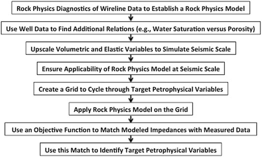
FIGURE A1. Interpretation flowchart.

References

Arévalo-López, H. S., and Dvorkin, J. P. (2016). Porosity, mineralogy, and pore fluid from simultaneous impedance inversion. Lead. Edge 35, 423–429. doi:10.1190/tle35050423.1

CrossRef Full Text | Google Scholar

Arévalo-López, H. S., and Dvorkin, J. P. (2017). Simultaneous impedance inversion and interpretation for an offshore turbiditic reservoir. Interpretation 5, SL9–SL23. doi:10.1190/int-2016-0192.1

CrossRef Full Text | Google Scholar

Backus, G. E. (1962). Long-wave elastic anisotropy produced by horizontal layering. J. Geophys. Res. 67, 4427–4440. doi:10.1029/jz067i011p04427

CrossRef Full Text | Google Scholar

Batzle, M., and Wang, Z. (1992). Seismic properties of pore fluids. Geophysics 57, 1396–1408. doi:10.1190/1.1443207

CrossRef Full Text | Google Scholar

Dvorkin, J., and Alabbad, A. (2019). Velocity-porosity-mineralogy trends in chalk and consolidated carbonate rocks. Geophys. J. Int. 219, 662–671. doi:10.1093/gji/ggz304

CrossRef Full Text | Google Scholar

Dvorkin, J. (2019). Diagenesis-driven pore fluid discrimination. Lead. Edge 38, 40–43. doi:10.1190/tle38050366.1

CrossRef Full Text | Google Scholar

Dvorkin, J., Gutierrez, M., and Grana, D. (2014). Seismic reflections of rock propertiesCambridge University Press.

CrossRef Full Text | Google Scholar

Dvorkin, J., and Alkhater, A. (2004). Pore fluid and porosity mapping from seismic. First Break. 22, 53–57.

CrossRef Full Text | Google Scholar

Dvorkin, J., and Nur, A. (1998). Acoustic signatures of patchy saturation. Int. J. Solid Struct. 35, 4803–4810. doi:10.1016/s0020-7683(98)00095-x

CrossRef Full Text | Google Scholar

Dvorkin, J. P. (2008). Yet another vs equation. Geophysics 73, E35–E39. ‏doi:10.1190/1.2820604

CrossRef Full Text | Google Scholar

Gassmann, F. (1951). Uber die elastizitat poroser medien. Viertel. Naturforsch. Ges. Zürich 96, 1–23.‏

Google Scholar

Hill, R. (1952). The elastic behavior of crystalline aggregate. Proc. Physic. Soc. A65, 349–354.

Google Scholar

Lau, A., Gonzalez, A., Mallick, S., and Gillespie, D. (2002). Waveform gather inversion and attribute-guided interpolation: a two-step approach to log prediction. Lead. Edge 21, 1024–1027. doi:10.1190/1.1518440

CrossRef Full Text | Google Scholar

Mallick, S. (2007). Amplitude-variation-with-offset, elastic-impedence, and wave-equation synthetics - a modeling study. Geophysics 72, C1–C7. doi:10.1190/1.2387108

CrossRef Full Text | Google Scholar

Mallick, S. (2001). AVO and elastic impedance. Lead. Edge 20, 1094–1104. doi:10.1190/1.1487239

CrossRef Full Text | Google Scholar

Mavko, G., Mukerji, T., and Dvorkin, J. (2020). Rock physics handbook. 3rd Edn. Cambridge, UK: Cambridge University Press, 396.

Monachesi, L. B., Wollner, U., and Dvorkin, J. P. (2020). Effective pore fluid bulk modulus at patchy saturation: an analytic study. JGR Solid Earth 125, 1–12. doi:10.1029/2019jb018267

CrossRef Full Text | Google Scholar

Raymer, L. L., Hunt, E. R., and Gardner, J. S. (1980). “An improved sonic transit time-to-porosity transform,” in SPWLA 21st annual logging symposium, society of petrophysicists and well-log analysts, Lafayette, Louisiana, July 08, 1980 (Lafayette, LA: ‏Society of Petrophysicists and Well Log Analysts), 1–13.

Google Scholar

Russell, B. (1999). Comparison of poststack inversion methods. SEG Tech. Program Expand. Abst. 10, 1–4. doi:10.1190/1.1888870

CrossRef Full Text | Google Scholar

Souvannavong, V., Allo, F., Coleou, T., Colnard, O., Machecler, I., Dillon, L., et al. (2013). “Petrophysical seismic inversion over an offshore carbonate field,” in International petroleum technology conference, Rio de Janeiro, Brazil, August 15–18 2013 Beijing, China: European Association of Geoscientists and Engineers, 1–5.

Google Scholar

Wollner, U., Arevalo-Lopez, H., and Dvorkin, J. (2017). Seismic-scale petrophysical interpretation and gas-volume estimation from simultaneous impedance inversion. Lead. Edge 36, 910–915. doi:10.1190/tle36110910.1

CrossRef Full Text | Google Scholar