 Rashmi Singh
 Prosanta Kumar Khan
- Department of Applied Geophysics, Indian Institute of Technology (Indian School of Mines) Dhanbad, Dhanbad, India
The Eastern Indian Shield (EIS) is comprised of the intracratonic (coal-bearing) Damodar Gondwana basin, rift-controlled extensional Lower Gangetic basin (LGB), and the downward flexed Indo-Gangetic basin (IGB). The present study involves the computations and mapping of the basement configuration, sediment thickness, Moho depth, and the residual isostatic gravity anomaly, based on 2-D gravity modeling. The sediment thickness in the area ranges between 0.0 and 6.5 km, and the Conrad discontinuity occurs at ∼17.0–20 km depth. The depth of the Moho varies between 36.0 and 41.5 km, with the maximum value beneath the Upper Gangetic basin (UGB), and the minimum of ∼36 km (uplifted Moho) in the southeastern part beneath the LGB. The maximum residual isostatic anomaly of +44 mGal in the southern part indicates the Singhbhum shear zone, LGB, and Rajmahal trap to be under-compensated, whereas the northern part recording the minimum residual isostatic anomaly of –87.0 mGal is over-compensated. Although the region experienced a few moderate-magnitude earthquakes in the past, small-magnitude earthquakes are sparsely distributed. The basement reactivation was possibly associated with a few events of magnitudes more than 4.0. Toward the south, in the Bay of Bengal (BOB), seismic activities of moderate size and shallow origin are confined between the aseismic 85 and 90°E ridges. The regions on the extreme north and south [along the Himalaya and the equatorial Indian Ocean (EIO)] are experienced moderate-to-great earthquakes over different times in the historical past, but the intervening EIS and the BOB have seismic stability. We propose that the two aseismic ridges are guiding the lithospheric stress fields, which are being further focused by the basement of the EIS, the BOB, and the N-S extended regional fault systems into the bending zone of the penetrating Indian lithosphere beneath the Himalaya. The minimum obliquity of the Indian plate and the transecting fault systems in the Foothills of the Himalaya channelize and enhance the stress field into the bending zone. The enhanced stress generates great earthquakes in the Nepal-Bihar-Sikkim Himalaya, and on being reflected back through the apparently stable EIS and BOB, the stress field creates deformation and great earthquakes in the EIO.
Introduction
Occasional incidents of major damaging earthquakes, such as 2015 (Mw 7.8) Nepal-Bihar, 2011 (Mw 6.9) Sikkim, 1988 (Mw 6.8) north Bihar, 1934 (Mw 8.0) north Bihar-Nepal, and 1833 (ML 7.6) Nepal-Bihar, account continued accumulation and occasionally release of strain energy in the Nepal-Bihar-Sikkim part of the Himalayas (Ansari et al., 2014; Khan et al., 2017a; Singh et al., 2020). The adjacent area of the Eastern Indian Shield (EIS) also experienced a number of moderate-magnitude earthquakes, such as 1868 (M5.7) Manbhum, 1868 (M 5.0) Hazaribagh, 1963 (M 5.0) Ranchi, and 1969 (M5.7) Bankura (Chandra, 1977; Kayal et al., 2009; Gupta et al., 2014; Rastogi, 2016). The earthquakes occurring in the EIS and adjacent areas (Figures 1, 2) are linked with the continued convergence of the Indian plate beneath the Himalaya (Khan et al., 2020; Singh et al., 2020). Toward the north, the Gangetic fore-deep, the Himalayan Frontal Thrust (HFT), West Patna Fault (WPF), East Patna Fault (EPF), and Munger-Saharsa Ridge Fault (MSRF) are the main structural discontinuities; these run either parallel or orthogonal to the southern border of the Nepal Himalaya (Figure 2). A few of these features, along with other transecting faults, have shown strike-slip dominated movements during the Holocene period (Sastri et al., 1971; Valdiya, 1976; Ansari et al., 2014; Khan et al., 2014; Singh et al., 2020). Such operative dynamics and kinematics toward the south of the Himalayan Foothills, compatible with the back propagation of the compressive stress field, facilitated deformation in the EIS, and the effects were likely extended up to the Central Indian basin (McKenzie and Sclater, 1971; Minster and Jordan, 1978; Stein and Okal, 1978; Gordon et al., 1990; DeMets et al., 1994).
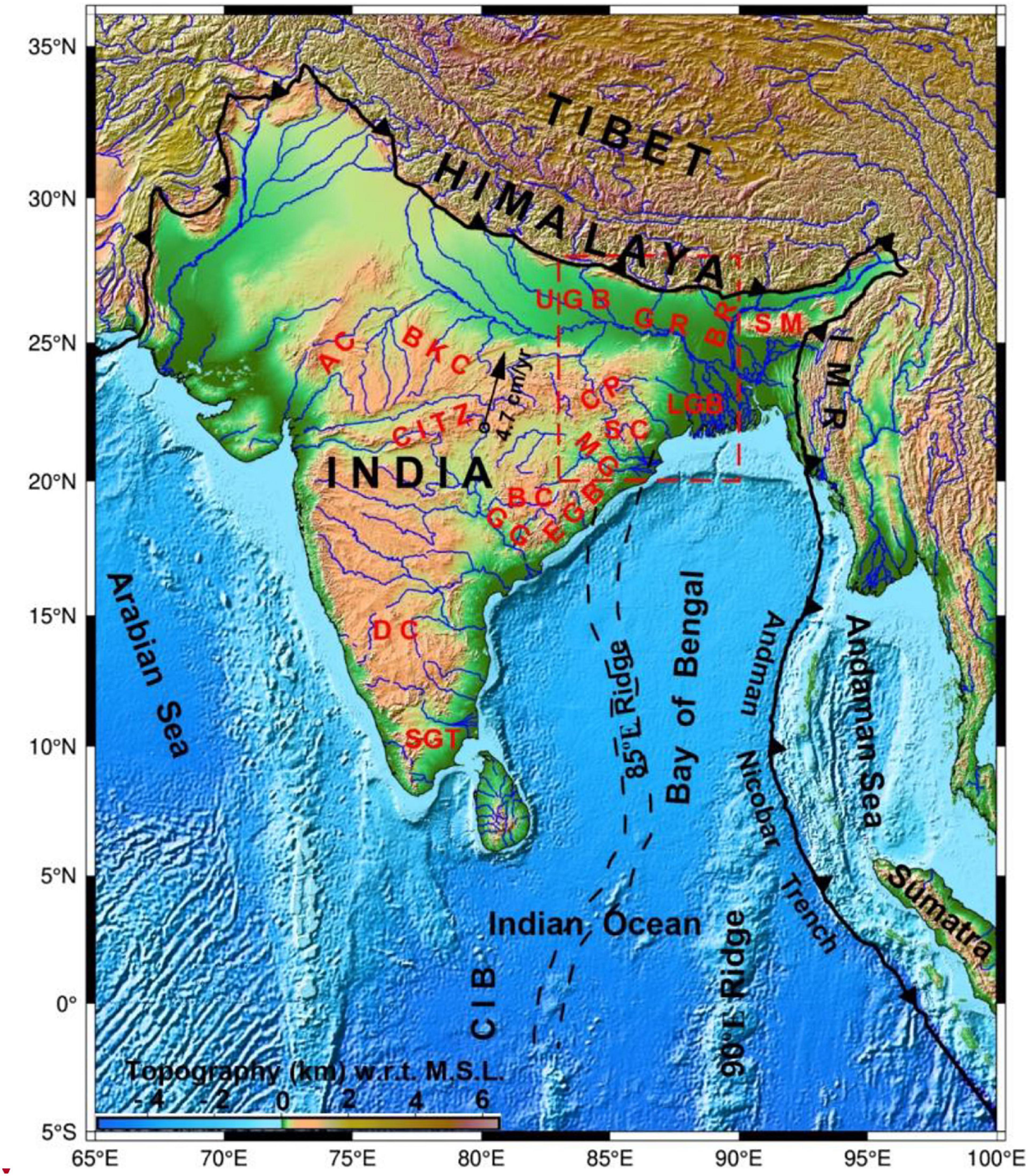
Figure 1. Regional map (reconstructed after Khan et al., 2017b; Valdiya and Sanwal, 2017; Altenbernd et al., 2020) showing the location of the study area (rectangular block demarcated by red dashed line). Abbreviations: AC, Aravalli Craton; BKC, Bundelkhand Craton; CITZ, Central India Tectonic Zone; EGB, Eastern Ghats Belt; CP, Chhotanagpur Plateau; SC, Singhbhum Craton, BC, Bastar Craton; DC, Dharwar Craton; SGT, Southern Granulite Terrain; MG, Mahanadi Graben; GG, Godavari Graben; SM, Shillong Massif; IMR, Indo-Myanmar Range; GR, Ganga River; UGB, Upper Gangetic Basin; LGB, Lower Gangetic Basin; BR, Brahmaputra River.
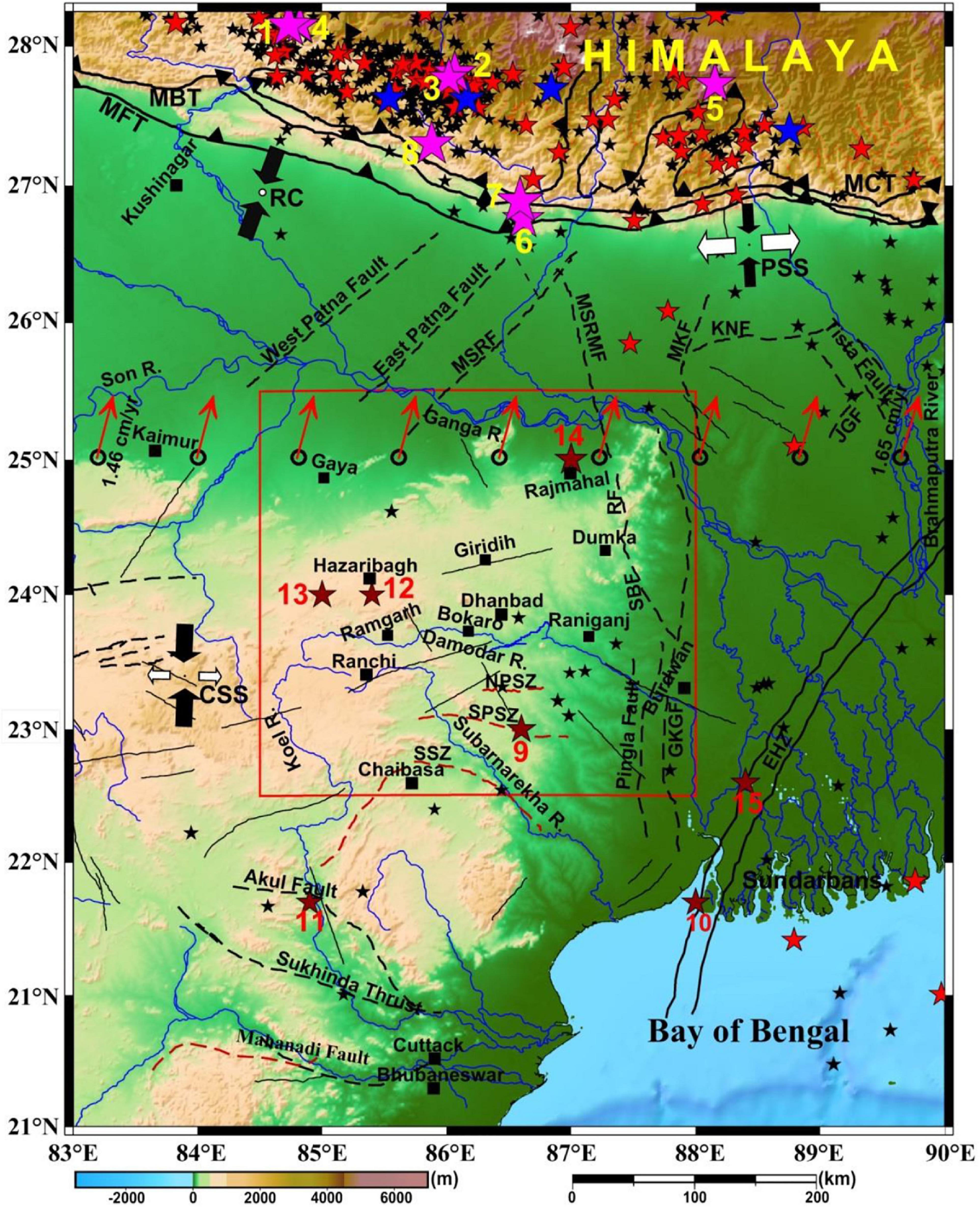
Figure 2. Seismoteconics and topographic relief Map of EIS (EIS) and adjoining regions (after Dasgupta et al., 2000; Singh et al., 2020). The study area is marked by a red rectangular box. Black dashed lines represent faults, and black solid lines denote lineaments. Blue solid lines show the various permanent rivers. Black solid squares represent the locations of a few important areas. A combination of black and white solid arrows shows the stress regimes of that part within shallow depth (0–20 km). RC, radial compression; PSS, pure strike-slip; CSS, compressive strike-slip. Red arrows represent the Indian plate velocity motion direction with respect to the Eurasian plate. All stars show the seismicity since 1973 to May 2020 (from USGS Catalog). Magenta stars show the location of damaging earthquakes with magnitudes of 6.5 < M ≤ 8.0 (1: 2015 M 7.8 Nepal, 2: 2015 M 7.3 Nepal, 3: 2015 M 6.7 Nepal, 4 2015 M 6.6 Nepal 5: 2011 M 6.9 Sikkim, 6: 1988 M 6.9 Nepal-India Border, 7: 1934 M 8.0 Nepal-India Border, and 8: 1833 M 7.6 Nepal-India Region). Maroon stars represent the location of historical earthquakes that occurred in EIS and nearby regions within 5 < M ≤ 6.3 (9: 1969 M 5.7 Bankura, 10: 1964 M 5.5 Midnapur, 11: 1963 M 5.2 Thethanagar, SE Bihar, 12: 1868 M 5.5 Manbhum, 13: 1868 M 5.0 Hazaribagh, 14: 1866 M 6.3 Bengal, and 15: 1861 M 5.7 Calcutta). Blue stars show the epicenter location of earthquakes between 6 and 6.5 magnitude, red stars represent earthquake location within 5 ≤ M < 6, while the black stars denote epicenter locations of earthquakes within 4 ≤ M < 5. Abbreviations: MFT, Main Frontal Thrust; MBT, Main Boundary Thrust; MCT, Main Central Thrust; MSRF, Munger-Saharsa Ridge Fault; MSRMF, Munger-Saharsa Ridge Marginal Fault; GKGF, Garhmayna-Khandaghosh Fault; SBF, Sainthia Bahmani Fault; MKF, Malda-Kishanganj Fault; JGF, Jangipur-Gaibanda Fault; KNF, Katihar-Nailphamari Fault; CGG, Chhotanagpur gneissic complex terrain; SSZ, Singhbhum shear zone; NPSZ, North Purulia shear zone; SPSZ, South Purulia shear zone; R., River.
The present study was undertaken at the core of the EIS, which occupies portions of four Indian states—Bihar, Jharkhand, Orissa, and West Bengal—to investigate the link between the regional geodynamic processes and earthquake occurrences. Besides the tectonic features mentioned above, the eastern part of the EIS is associated with the Rajmahal Trap and several faults striking N-S (e.g., Pingla fault, Sainthia Bahamani fault, and GKGF faults). The core (central part) of the EIS has ∼ E-W striking regional shear zones such as the North Purulia, South Purulia, and Singhbhum (Figure 2). Thus, the area is tectonically very important for its location, and is essentially a geological corridor to the Eastern Himalaya and the Indo-Myanmar Ranges. The present study therefore was carried out to delineate the basement configuration and the Conrad and Mohorovičić (Moho) discontinuities based on analysis of the gravity anomalies. The detailed gravity modeling and mapping and the historical earthquake data available for the region were used for exploring the level of seismic stability at different locations of the study region.
The Moho depth for several small blocks of the EIS was determined by several studies (Choudhury, 1974; Verma et al., 1976, 1980; Bhattacharya and Shalivahan, 2002; Singh et al., 2004, 2015; Kayal et al., 2011; Sharma et al., 2015). All these investigations were constrained by an insufficient coverage of dataset and smaller sizes of the areas. The outcomes of these investigations provide valuable information regarding the crustal structure (discussed below).
The residual gravity analysis over the Raniganj Coalfield area (∼6 × 10³ km2) shows a gravity low of around –32 mGa1 associated with the Gondwana sediments, with a maximum estimated sediment thickness of ∼2 km (Verma et al., 1976). Gravity field analysis of North Singhbhum (∼36 × 103 km2 area) could delineate the Bouguer anomalies of +4 to −62 mGal, with the estimated thickness of the basin, based on a 2D gravity model, of about 6–7 km (Verma et al., 1980). An analysis of free air, Bouguer, and isostatic anomalies over a part of the shield near the Gaya region shows a 6.6 km thick sediment layer underneath the Lower Gangetic basin (LGB). Compiling datasets from a few stations, a crustal thickness of 42.5 km underneath the northern part of the shield, 31.5 km underneath the Indo-Gangetic basin (IGB), and 81 km underneath the Higher Himalaya of Nepal-Bihar region were also estimated by Qureshy (1969). While the Bouguer gravity analysis, carried out by Choudhury (1974), for the Indo-Gangetic Plain and the northern Himalayan region, shows a crustal thickness of ∼35–37 and ∼70–72 km, respectively. A magnetotelluric study reports 40 km deeper Moho beneath the Singhbhum granite and adjoining regions (Bhattacharya and Shalivahan, 2002). Receiver function analysis of P-wave gives a depth of ∼41–42 km for the Moho and ∼20 km for the Conrad discontinuity below the IIT (ISM), Dhanbad seismic station (Kayal et al., 2011; Sharma et al., 2015). A 2D gravity modeling study shows that the Moho depth varies from ∼38 km below the Rajmahal Traps to ∼40 km near the Raniganj region (Singh et al., 2004). Lithospheric 3D mapping of the EIS shows that the Moho ranges from ∼35 to 40 km near Mahanadi, Damodar, and LGB (Singh et al., 2015). For a regional scale, Bouguer gravity anomalies can reflect the changes in mass disseminations between the lower crust and the upper mantle, and the isostatic stability (Tealeb and Riad, 1986). Bouguer anomalies and surface relief are also closely connected with the crustal thickness (Coron, 1969; Woollard, 1969; Pick et al., 1973; Riad et al., 1983; Riad and El-Etr, 1985). In the present study, the Bouguer gravity anomaly data and the geophysical parameters of various studies (Choudhury, 1974; Verma and Ghosh, 1977; Verma, 1985; Singh et al., 2004) were used to deduce the regional structural framework of the shallow basement, overlying sedimentary cover, and the Conrad and Moho discontinuities. The present study also attempts to visualize the crustal balance in terms of isostasy. Isostatic study of continents accounts for the mechanical balance of lithosphere at the time of loading (Watts et al., 1980; Djomani et al., 1992) and links to the deep-density structure, providing constraints on the geological model (Simpson et al., 1986).
Tectonic Set-Up
The study area comprises the northern portion of the Singhbhum craton, the Chhotanagpur gneissic complex, and the southern portion of the Himalayas (Figure 1). The area is bounded by the Eastern Ghats mobile belt on the south and the Himalayan foothills on the north. The Gangetic alluvium and the Quaternary sediments of LGB border its eastern part, whereas the western part is bordered by the Gondwana sediments of the Sone-Mahanadi basin. The Upper Jurassic to lower Cretaceous basalts form the Rajmahal Traps, at the contact zone of the Chhotanagpur Gneiss Complex and the LGB. The Ganges River flows all along the north of the study area and was evolved during the bending of the Indian plate beneath the Himalaya (Figures 1, 2). The rivers Subarnarekha and Koel pass through the southern part of the area, whereas the coal-bearing, faulted Damodar Valley transects the central part of the region from west to east.
The study area has variable relief, with the highest elevation in the Ranchi Plateau, situated at ∼610–1097 m from mean sea level (MSL) (Pandey et al., 2013). Several dissected hills with a number of hill stations constitute the adjacent Hazaribagh Plateau drained by the Damodar valley. The Chhotanagpur Plateau and the Hazaribagh Plateau have outcrops of gneisses, schists, and granite of Precambrian rocks (Ghose, 1983). Some other plateaus, like Kaimur Plateau and Rajmahal Hills, can be differentiated from each other by steep and narrow slopes known as scarps.
Mutual cyclic interactions of two converging microplates, i.e., Singhbhum and Chhotanagpur (Sarkar, 1982), during the Proterozoic times facilitated subduction, rifting, mantle plume activities, and mafic magmatism in the region (Pandey and Agarwal, 1999; Bose, 2008). The cyclic interactions happened in three consecutive stages with intervening quiescence (Sarkar, 1982), which further simplified the isostatic adjustments with coeval upliftment with intrusions of basic dyke swarms, erosion, and paralic sedimentation (Bose, 1999, 2009). During the Precambrian, the northward movement of the Singhbhum block toward the continental margin of the Chhotanagpur block produced a consuming plate boundary (Figure 1). The compressional stress produced by the plate merging caused N-S crustal shortening, resulting in the upliftment on the Chhotanagpur granite-gneissic terrain and beginning the basement reactivation and fresh rupture development (Sarkar and Saha, 1977).
The Chhotanagpur peneplain has been uplifted three times during the Cenozoic due to the flexural responses caused by the subduction of the Indian lithosphere toward the southern edge of the Himalayas, and gave rise to some familiar waterfalls, like Jonha and Hundru, on the scarps. During the Eocene to Oligocene period the first upliftment took place, forming the Pat region; the second one happened during the Miocene period which developed the Ranchi and Hazaribagh Plateau; and the third one took place during the Pliocene and Pleistocene period, which caused upliftment of the outer Chhotanagpur Plateau (Naqvi and Rogers, 1987; Weaver, 1990).
The Chhotanagpur plateau is comprised of high-grade gneisses and migmatites containing enclaves of meta-sediments, and mafic and ultramafic rocks. The basement of the Chhotanagpur plateau is represented by an uncategorized gneissic complex. Systems of Proterozoic fold belt occur as secluded patches within the Chhotanagpur Granite Gneissic terrain. Later, during late Palaeozoic and Mesozoic, Gondwana sediments were deposited in linear grabens in the Damodar valley. Irregular sedimentation above crystalline metamorphic rocks, harmonized subsidence, and sprinkled periodic accumulation of coal measures were greatly conditioned by climatic variation in the period of sedimentation in the Gondwana basin in the eastern part of the EIS (Sarkar, 1982). The maximum thickness of sediment filling in the basin is estimated to be 2.9 km in the central part (Verma et al., 1980). Intermittent periods of faulting and epeirogenic uplift of the margins of the master basin dismembered the master basin into several smaller sub-basins (Mahadevan, 2002). Various hot springs with numerous features are broadly dispersed over this area, and the area is apparently associated with several fault zones (Mahadevan, 2002). The Chhotanagpur Granite–Gneiss Complex (CGGC) mainly consists of granitic gneisses, migmatized porphyritic granite, and many meta-sedimentary enclaves. The Central CGGC gneisses and the western CGGC granites show almost similar ages of 1.7 Ga, whereas the migmatites and granulites, and granitic gneisses of northeastern CGGC (Dumka area), show ages of 1.5–1.6 Ga (Chatterjee et al., 2008).
Data and Methodology
Gravity Modeling and Validation
Gravity modeling is an important tool for delineation of crustal structures. Gravity data show an ordered link between crustal structure, density, and the surface altitude. In this line, a Bouguer anomaly map was reconstructed for the area covering a part of the Gangetic basin and EIS (i.e., between 22.5–25.5°N latitude and 84.5–88°E longitude) compiling the data from the second generation gravity map series of India (GMSI, 2006). An inaccuracy of about ± 0.5 mGal for the errors in elevation of 2–3 m was achieved in these data. The area of the new Bouguer anomaly map (Figure 3) has been divided into 99 square-grids, with a dimension of 1° × 1°. A shifting window with 75% overlapping area is used for inherent continuity of the data points and better resolution for delineating the basement and the Conrad discontinuity of the study area.
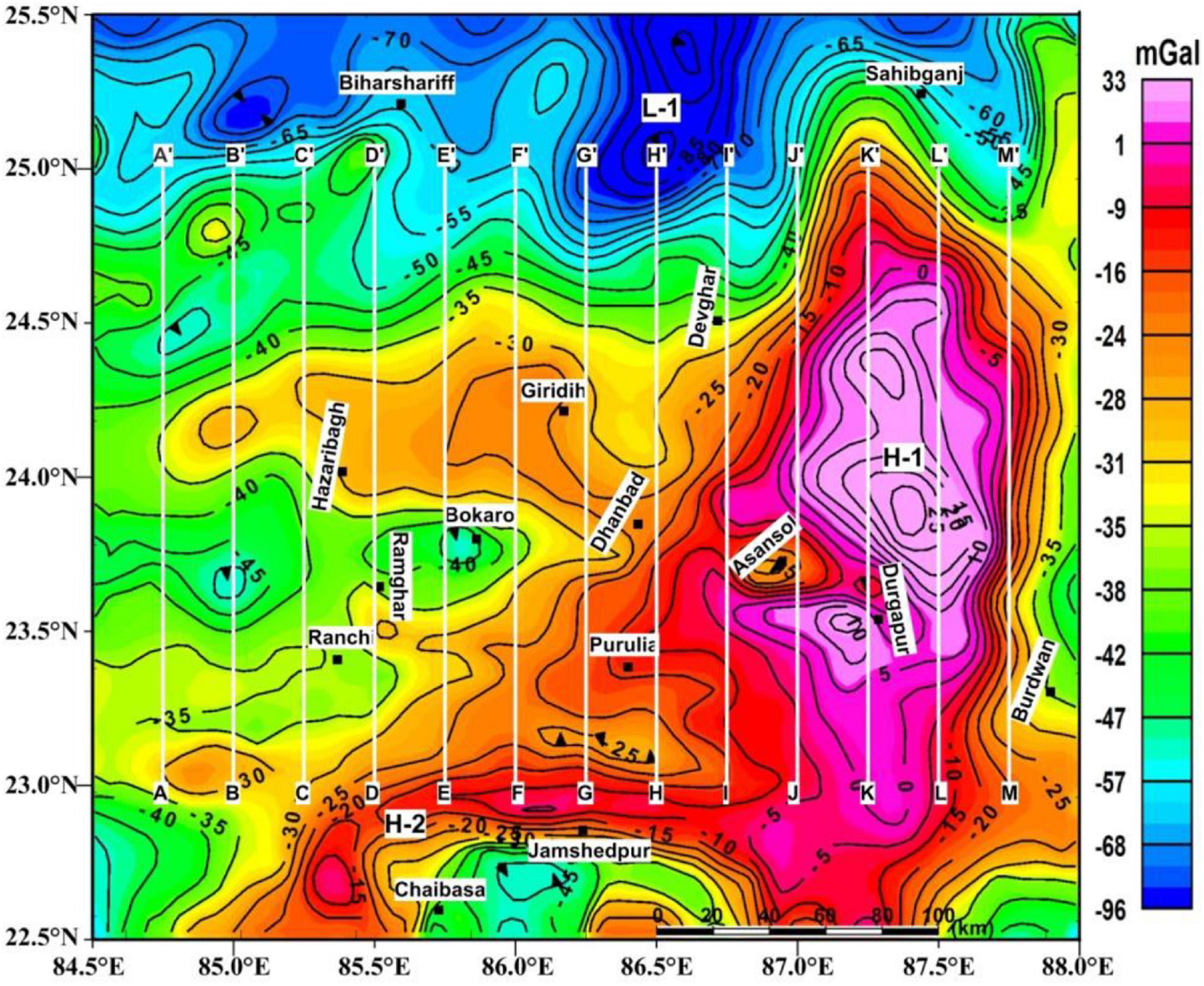
Figure 3. Bouguer gravity anomaly map of the study area reconstructed from GMSI (2006). White vertical solid lines are the profiles, taken for the 2D gravity modeling. H-1 and H-2 represent the area associated with high Bouguer gravity anomalies, and L-1 represents the area with low Bouguer gravity anomaly.
The Moho depth was computed by the spectral analysis (Figure 4) (Odegard and Berg, 1965; Bhattacharyya and Leu, 1975) over 12 blocks, by dividing the Bouguer anomaly map into smaller areas of dimension of 2° × 2° in an overlapping adjacent grid. We have also computed the Moho depth based on the Airy-Heiskanen model at the same grid for better resolution and insufficient data points, as the GMSI (2006) gravity map is created from a grid of dimension 5.5 × 5.5 km2. The 2D inverse gravity modeling was performed by adding layers incorporating its prior information as explained in Figure 5 and Table 1. Error minimization between the observed and calculated gravity anomalies was followed at various steps of the iteration processes, to optimize the gravity model.
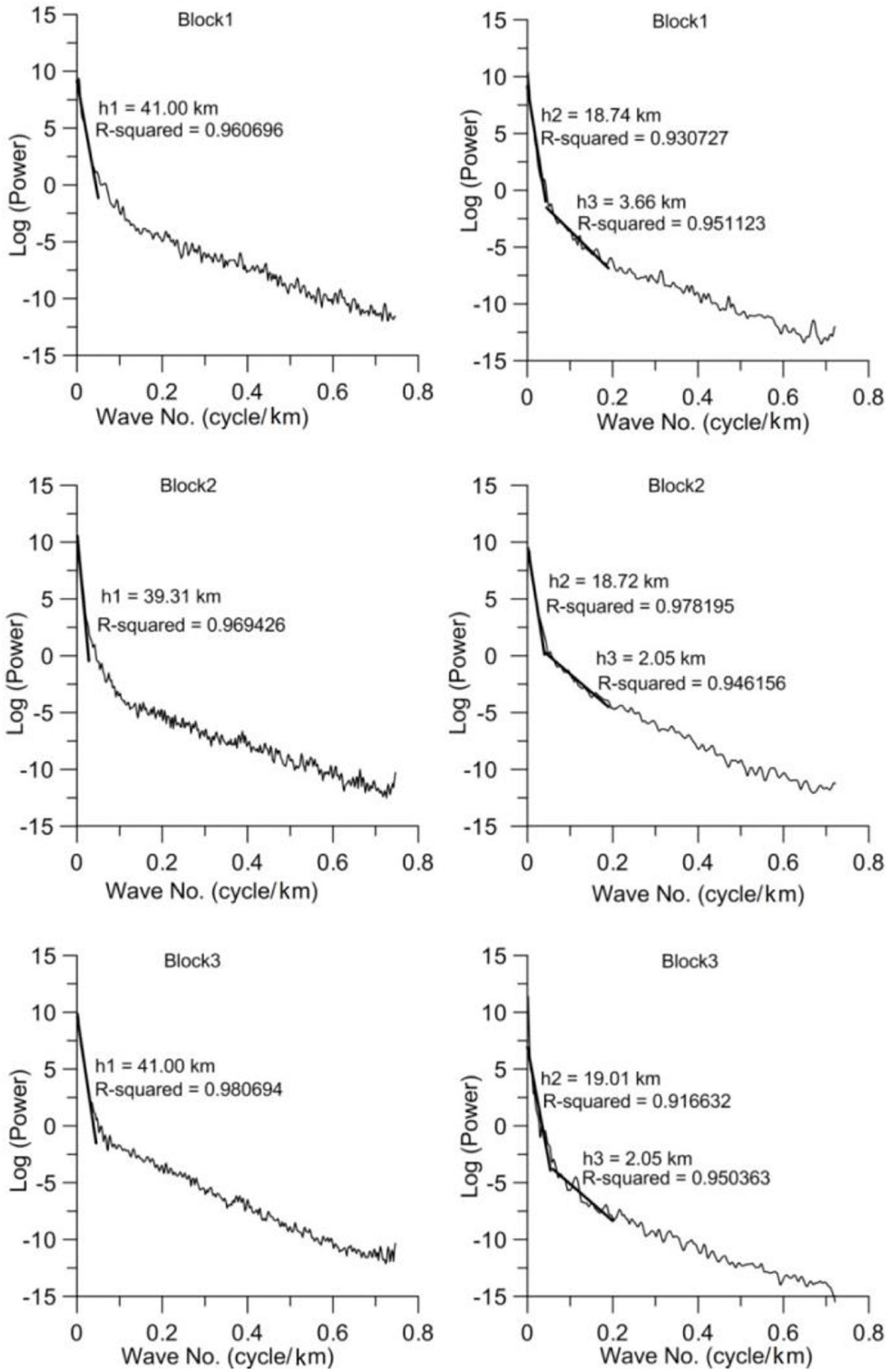
Figure 4. Spectral analysis plots illustrating the estimation of interface depths at different grids. Wave number is plotted on the X-axis, and the corresponding power spectra of gravity are plotted on the Y-axis. Values of deepest density interface show Moho depth, and the shallowest interface shows sediment thickness.
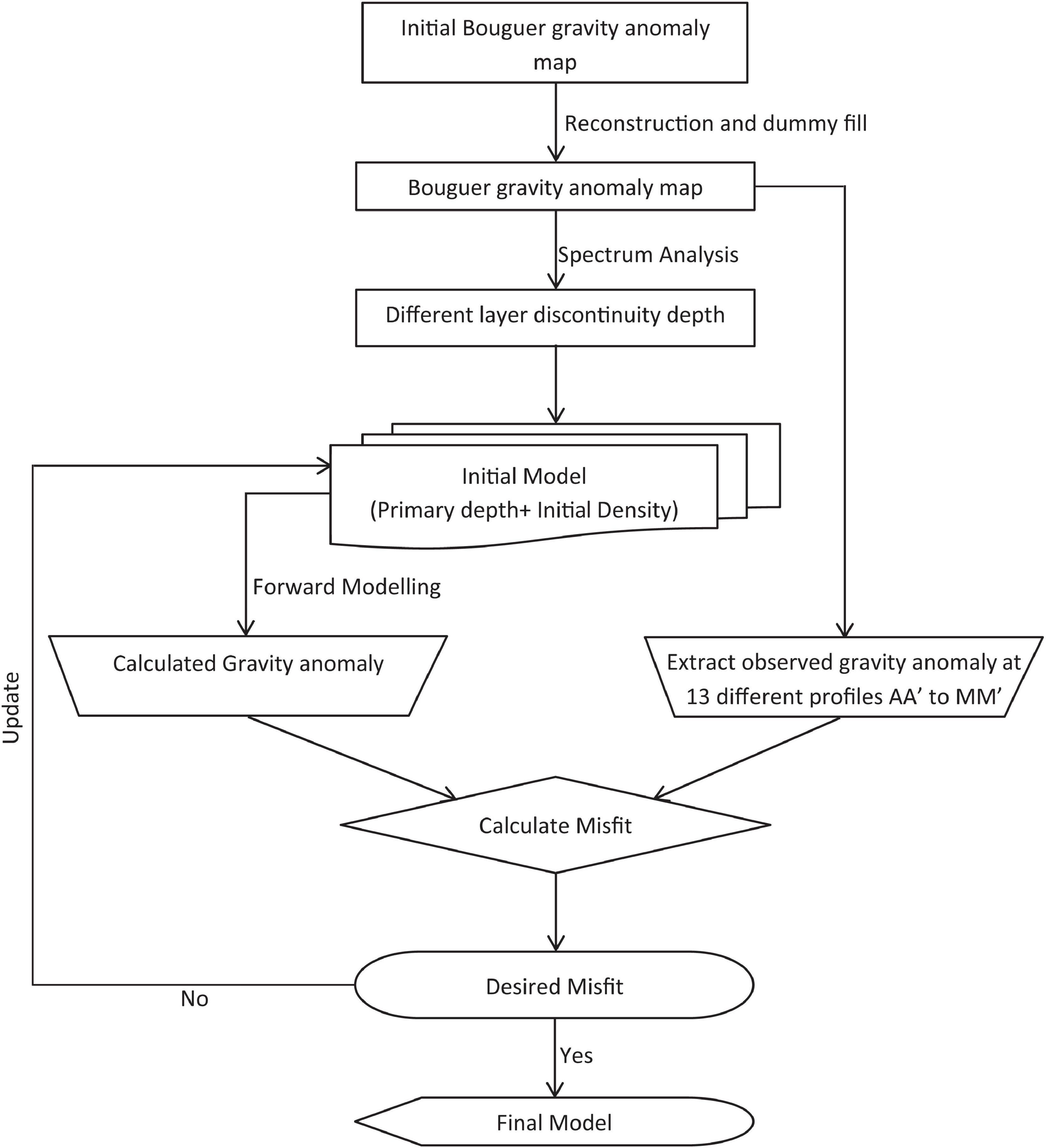
Figure 5. Flowchart showing the various steps followed for the gravity modeling.
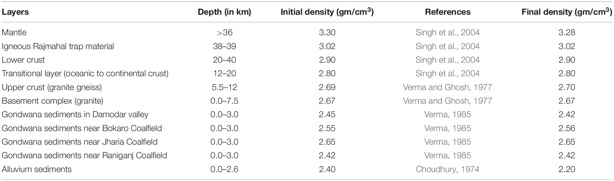
Table 1. Density used in the 2D gravity modeling.
The inverse gravity modeling using Geosoft was done along 13 profiles, considering various Earth models (Choudhury, 1974; Verma et al., 1976; Verma and Ghosh, 1977; Verma, 1985; Singh et al., 2004). Power spectrum analysis was carried out to compute depths of the sharp density discontinuities appearing at the basement, Conrad, and Moho. The efficacy of this method has been demonstrated in the literatures (Spector and Grant, 1970; Green, 1972; Curtis and Jain, 1975; Tselentis et al., 1988; Djomani et al., 1992; Chavez et al., 1999; Ates and Kearey, 2000; Lefort and Agarwal, 2002; Rivero et al., 2002; Carbó et al., 2003; Gomez-Ortiz et al., 2005; Bansal et al., 2006). We have computed the crustal discontinuities based on the spectral analysis (Figure 4) of the Bouguer gravity field. The Moho depth (Table 2) has been computed from the slope of the energy spectrum at the lower end of the wave-number band, while the basement depth (Table 3) has been computed at a slightly higher wave-number band. Interface depths with different density contrasts are computed using the following equation:
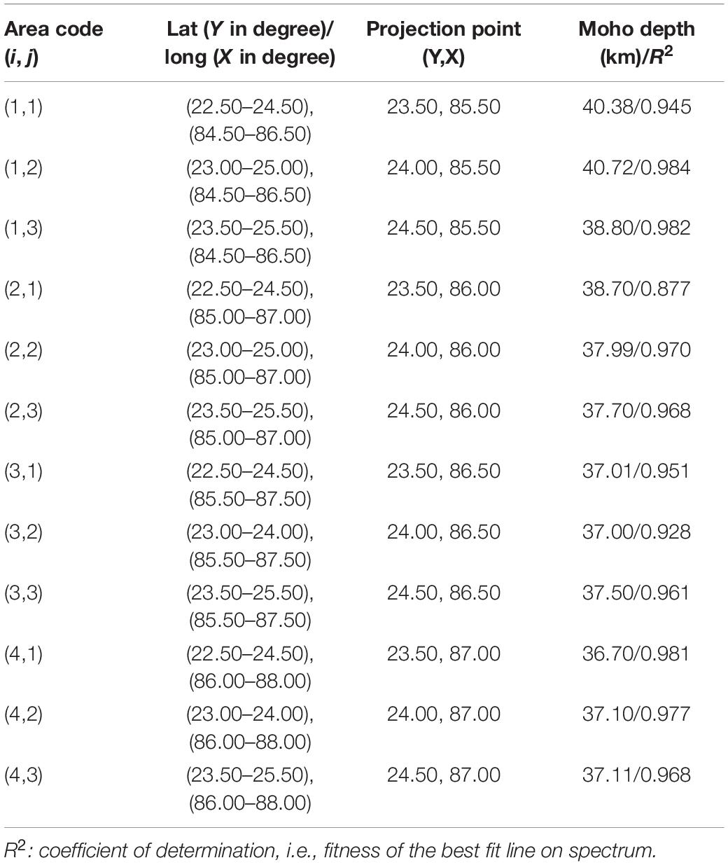
Table 2. 12 blocks of 2°×2° grid with a 75% overlap with the adjacent grid for Moho depth calculation.
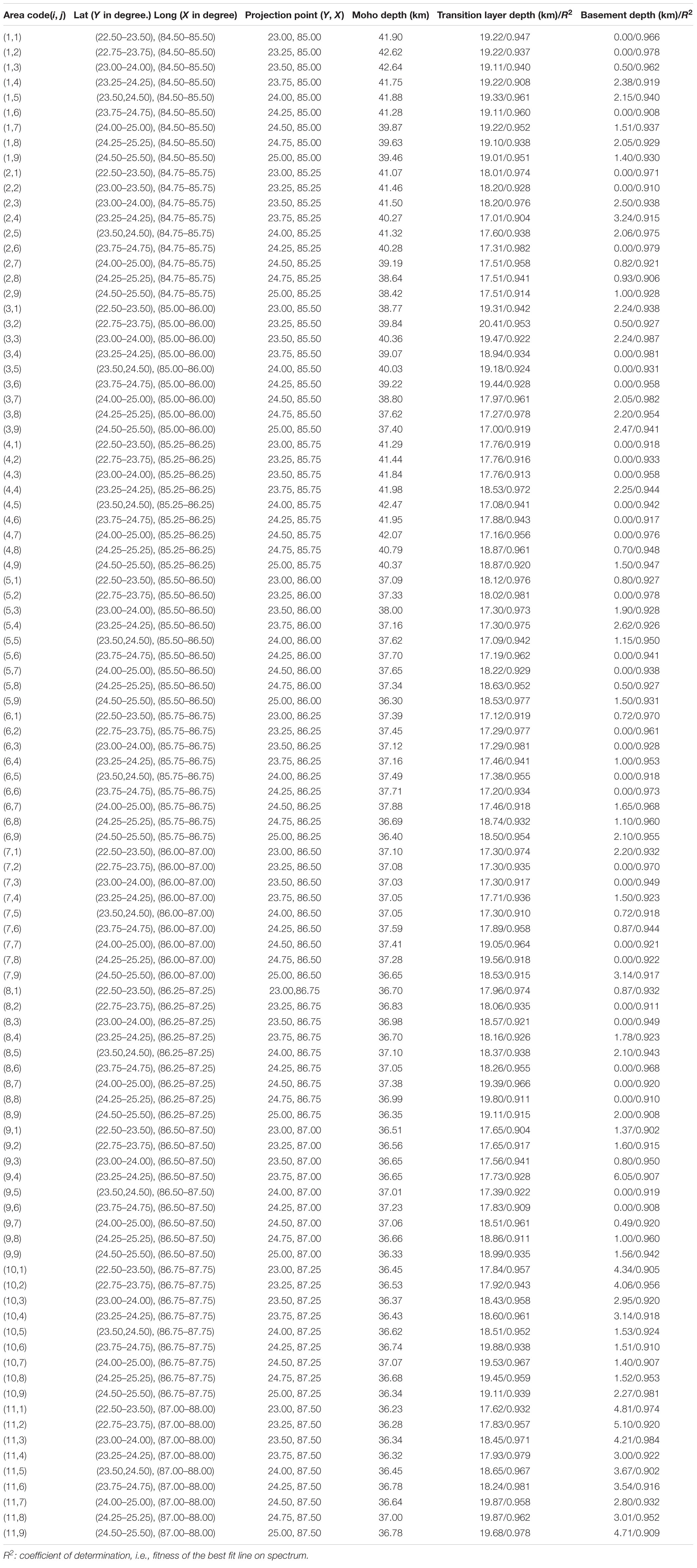
Table 3. Ninety-nine blocks of 1° × 1° grid, with a 75% overlap with the adjacent grid for basement and Conrad depth calculation.
where h is the average interface depth and E1 and E2 are the power in the spectrum at wave-number (cycles/km) k1 and k2 (cf. Spector and Grant, 1970; Karner and Watts, 1983; Maus and Dimri, 1995; Indriana, 2008; Bansal and Dimri, 2010; Chamoli et al., 2010).
Most of the geophysical methods, particularly the spectral analysis of potential field data, isostasy analysis, inversion of potential field data, receiver function, and seismic tomography, used for modeling and interpretation purposes, have some limitations as well as advantages. 2-D spectral analysis usually delivers spatially averaged depth for an undulated plane, i.e., an interface where density changes sharply, and depends on the gridding size of the data (Tselentis et al., 1988). In frequency domain, gravity anomalies generated from a multilayered source can be separated from each other by their own segments with the help of gravity anomaly spectrum and interpreted for the mean depth of the interface (Chamoli and Dimri, 2010). However, the spectral peak for each buried mass at different depths is not always sharp, and the overlapping of such peaks occasionally introduces ambiguity in the result. Refinement of higher wave-number components from noise is sometimes difficult due to its smaller amplitude, and the information loss can be minimized to < 10% by taking care of the window size of four to five times of the source depth (Regan and Hinze, 1976).
The Airy-Heiskanen isostatic technique results in reliable image gravity data on a continent-wide scale for the purpose of regional geologic interpretations. Isostatic residual gravity further enhances the short-wavelength anomalies produced by bodies at or near the surface and emphasizes the regional fabrics and trends in the gravity field. Isostatic anomaly gives information about the lateral mass distribution within the crust and mantle, having some geological interest (Simpson et al., 1986). However, crustal density variations are not considered for one fixed density for the entire crust. Gravity data alone cannot reveal the density inhomogeneity in the locally compensated crust. A solely isostatic model cannot provide the root geometry for a large continental region. There may be errors of less than 2 mGal in the calculation of isostatic residual anomaly because of the uncertainty present in gravity measurement, terrain correction, and station elevation (Chapin, 1996). The anomalies near the flanks are affected by the anomalies present at its neighborhood and become difficult to distinguish.
Gravity inversion method is well known for the derivation of appropriate anomalies due to Moho deflection (Prasanna et al., 2013), and its useful technique to detect Moho depth especially in a region where the availability of seismic data is insufficient. Moho interface can be delineated with the help of an iterative process (Shin et al., 2007). However, the filtering of wavelength effects of gravity from crustal inhomogeneities and deep-seated sources is difficult and complex. Inhomogeneities in the intra-crustal density or noise can create a stability problem in inversion and provide a wrong estimation of depth.
Seismic receiver function is a simple and unambiguous method for the detection of 1D crustal structure beneath the seismic station. Receiver function consists of direct, reflected, and converted phases of seismic wave trains (Burdick and Langston, 1977; Ammon et al., 1990; Das et al., 2019). Converted phases and shallow surface multiples carry average crustal information about the surrounding of the receiver station. However, this method can only be applied to a nearly horizontal layer and works best for low incidence angles of seismic rays. Regionalization of Moho depth (2D crustal structure) estimation needs highly dense seismic networks. The seismic tomography can give the information of velocity structures, seismotectonics, and characterization of the source area for tectonically complex regions (Zhao et al., 1992). It gives a high-resolution image of the earth’s interior. It can image the structures with different physical properties. Seismic tomography can also be done using surface waves and full waveforms (Geller, 1991; Iyer and Hirahara, 1993). However, the resolution of seismic tomography depends on the wavelengths of seismic waves. Since a longer wavelength is used, deeper sources can be imaged, but small features cannot be resolved. Tomography results are also non-unique and need a good coverage of seismic stations with a huge amount of earthquake data, and hence are suitable for seismically active regions.
The EIS region is not very seismically active, and is located to the south of the seismically active Himalayan orogen. Thus, a good coverage of seismic network will be essential for delineation of the regional crustal structure of the study area. Ambient noise tomography is also another option for the detection of crustal structures in a seismically stable region like EIS region; however, it needs a dense network of seismic stations. Thus, the present results of gravity modeling were partially validated by the receiver function studies (Mandal and Biswas, 2016), and complied by the gravity study of Singh et al. (2015). Only two broadband seismic stations, located in the Chhotanagpur plateau, have been operative since 2007: Dhanbad [run by IIT (ISM)] and Bokaro [run by National Centre of Seismology (NCS), New Delhi]. The 1D crustal structure beneath Dhanbad and Bokaro stations has been estimated by several researchers using different initial velocity structures through receiver function analysis. Das et al. (2019) found 43 and 44 km crustal thickness beneath Dhanbad and Bokaro stations. Kosarev et al. (2013) found Moho at a 45 km depth beneath the Bokaro station. Kumar et al. (2013) found 42 km depth for the Moho below this station. Kayal et al. (2011) found a depth of 41 km for the Moho beneath the Dhanbad station, whereas Kumar et al. (2001) found highly complicated crust below the Bokaro station with a Moho depth of 54 km. This wide variability of Moho depth was possibly due to considering the same Vp/Vs or Poison’s ratio for the entire crust. The Moho depth computed under the present study varies from 37 to 41.5 km for the Chhotanagpur plateau and is ∼4–5 km shallower in comparison with the seismic methods. However, the Moho depth of ∼39 km near the Hazaribagh region (24.07°N and 85.38°E), ∼39.5–40 km in Ranchi (23.43°N and 85.43°E), and ∼40 km near Dumka (24.6°N and 87.08°E) are well correlated with the analysis of Mandal and Biswas (2016) (Table 4).
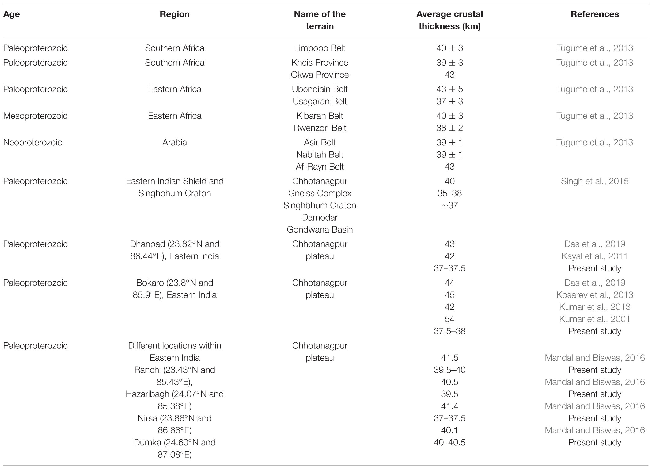
Table 4. Thickness of the crust of different shield areas around the globe and the present study area.
We use the Airy-Heiskanen model for the calculation of initial Moho depth assuming that the crust is isostatically being compensated. The isostatic imbalance and the delineation of many layers in the crust might be showing differences in Moho depth between the present study and results of receiver function studies. It is also found that the crustal structures obtained from seismic and gravimetric method are quite different depending on the geological and geophysical hypotheses, as well as different datasets (Reguzzoni et al., 2013). For example, well-known receiver function analysis starts their initial model by assuming a constant velocity and Vp/Vs, taking either a single or double layer of the crust for the calculation of 1D crustal structure (Dueker and Sheehan, 1997; Zhu, 2000; Zhu and Kanamori, 2000; Thompson et al., 2010; Kayal et al., 2011; Sharma et al., 2015; Mandal and Biswas, 2016; Song et al., 2017; Das et al., 2019). An incorrect or different initial seismic model may produce different or inaccurate crustal images, especially in the presence of heterogeneous medium with lateral velocity variations (Das et al., 2019). The calculation of crustal structure using the gravimetric method based on local and regional effect of Earth’s crust provides important outputs (Woollard, 1969; Tsuboi, 1979; Chapin, 1996).
Isostasy Analysis
According to the theory of isostasy given by the Airy model, the excess mass or root zone around the base of the crust normally supports the topography. Regional-scale low-amplitude and long-wavelength anomalies are often observed in hilly terrain and near the continental shelves (i.e., edges of continents), and are often masked by anomalies due to upper crustal structures (Simpson et al., 1986). Enhancement of gravity anomalies by removing topography-induced regional effects caused by shallow geologic features is done by routine use of polynomial fitting or wavelength-filtering method. The main objectives of most kinds of geologic and tectonic studies are the density distribution in the upper crust and are more precisely revealed by isostatic residual gravity anomaly maps than any other gravity maps. Qureshy and Warsi (1980) and Kumar et al. (2020) reconstructed the Airy-Heiskanen isostatic anomaly map over the Indian shield and adjoining regions using the world gravity map (Bonvalot et al., 2012). Several other workers reconstructed the isostatic anomaly maps for the Himalayas and IGB (Qureshy, 1969), Ninety-East Ridge (Tiwari, 2003), Deccan Trap (Qureshy, 1981), and for the Indian continent (Mishra et al., 2004). However, this is the first attempt to reconstruct the isostatic anomaly map for the EIS and adjacent regions using land gravity data (GMSI, 2006). Airy isostatic anomalies were computed from the difference between the gravity effect of topography and a crustal root from the Bouguer corrected anomaly, with the Parker (1972) series up to degree 4 to take care of the nonlinear effects (e.g., Lyons et al., 2000). We fixed the Moho depth to 38 km and formed an average of the spectrum analysis result. The density contrasts between surface and MSL and between mantle and crust are presumed to be 1470 and 400 kg/m3, respectively.
Gravity Profiling and Crustal Layer Mapping
The depths to the gravity sources in the sub-surface can be estimated from the shapes of the anomalies or the shapes of the power spectra (Figure 4) computed from the potential field data (Spector and Grant, 1970; Curtis and Jain, 1975; Djomani et al., 1992; Chavez et al., 1999; Lefort and Agarwal, 2002; Rivero et al., 2002; Gomez-Ortiz et al., 2005; Bansal et al., 2006). 2D spectral analysis for 1° × 1° and 2° × 2° to ensemble basement, Conrad depth, and Moho depth was carried out for archiving reliable information of the subsurface (Tables 2–4).
In the present study, 13 gravity profiles (AA′ to MM′, Figure 3) were selected to investigate the configurations of the crustal layers. Most of the profiles are orthogonal to the regional trend of the gravity anomaly. These profiles run from south to north, extending over ∼225 km, and were selected following the general structural trends of the various shear zones, except profiles 3–4 on the east, which are parallel to the trend of the Bouguer gravity anomaly. Profiles 1–4 (AA′ to DD′, Figure 6), located over the low Bouguer gravity anomaly (−35 to −60 mGal), are associated with the Ranchi-Hazaribagh plateau and UGB, while the profiles 9–13 (II′ to MM′) lie over the highest Bouguer gravity anomaly (i.e., −20 to +33 mGal), associated with the Rajmahal Trap and surrounding areas. The initial model along profiles AA′ to II′ was considered on the basis of spectrum analysis, studies of Verma et al. (1976); Verma (1985), Ismaiel et al. (2019), and Krishna et al. (2019), and other geological background data (Mahadevan, 2002). The final model was selected through minimization of error during optimization of the layer parameters and corresponding densities.
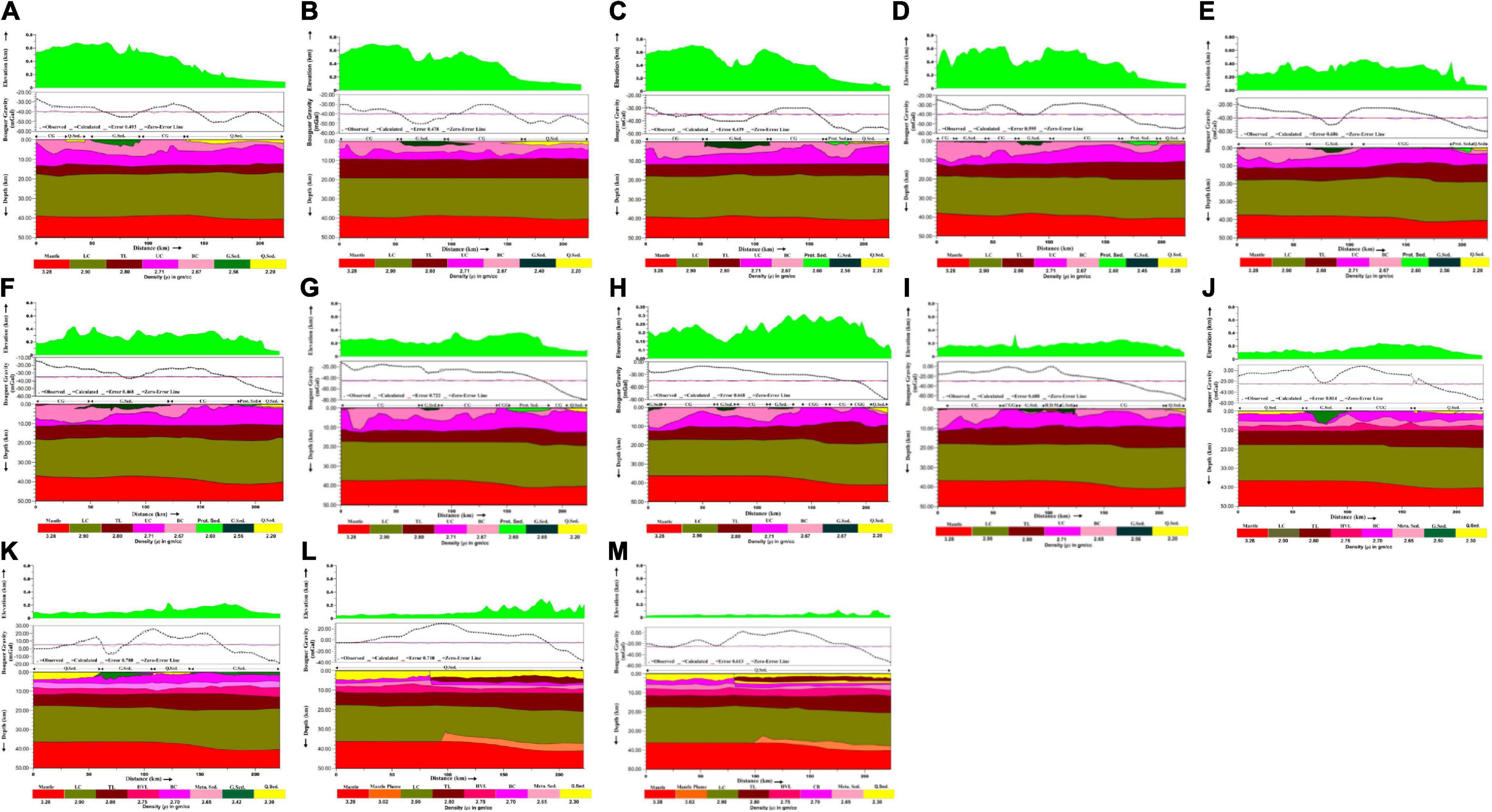
Figure 6. (A) 2D gravity model along profile AA′ (at longitude 84.75°E), location of the profile is shown in Figure 3. Abbreviations: CG, Chhotanagpur granite; CGG, Chhotanagpur granite gneiss; Q. Sed., quaternary sediment; G. Sed., Gondwana sediment; Prot. Sed., proterozoic sediment; LC, lower crust; TL, transition layer; UC, upper crust; BC, basement complex. (B) 2D gravity model along profile BB′ (at longitude 85.00°E), location of the profile is shown in Figure 3. (C) 2D gravity model along profile CC′ (at longitude 85.25°E), location of the profile is shown in Figure 3. (D) 2D gravity model along profile DD′ (at longitude 85.50°E), location of the profile is shown in Figure 3. (E) 2D gravity model along profile EE′ (at longitude 85.75°E), location of the profile is shown in Figure 3. (F) 2D gravity model along profile FF′ (at longitude 86.00°E), location of the profile is shown in Figure 3. (G) 2D gravity model along profile GG′ (at longitude 86.25°E), location of the profile is shown in Figure 3. (H) 2D gravity model along profile HH′ (at longitude 86.50°E), location of the profile is shown in Figure 3. (I) 2D gravity model along profile II′ (at longitude 86.75°E), location of the profile is shown in Figure 3. (J) 2D gravity model along profile JJ′ (at longitude 87.00°E), location of the profile is shown in Figure 3. (K) 2D gravity model along profile KK′ (at longitude 87.25°E), location of the profile is shown in Figure 3. (L) 2D gravity model along profile LL′ (at longitude 87.50°E), location of the profile is shown in Figure 3. (M) 2D gravity model along profile MM′ (at longitude 87.75°E), location of the profile is shown in Figure 3.
The 2D gravity modeled parameters for the study area (84.75–87.75°E and 23.0–25°N) covered by all the 13 profiles (AA′ to MM′) were used for the computation of parameters of different crustal layers. The results of the 2D gravity modeling were integrated into two maps for the Moho discontinuities and sediment thickness mapping (Figures 7, 8). The mapping of the Conrad discontinuity was not carried out because of its apparent uniformity over the area. The isostatic anomaly (Figure 9) was computed based on the differences between the Bouguer gravity anomalies and the gravity values of the computed root zones estimated from the topography (Heiskanen and Vening Meinesz, 1958).
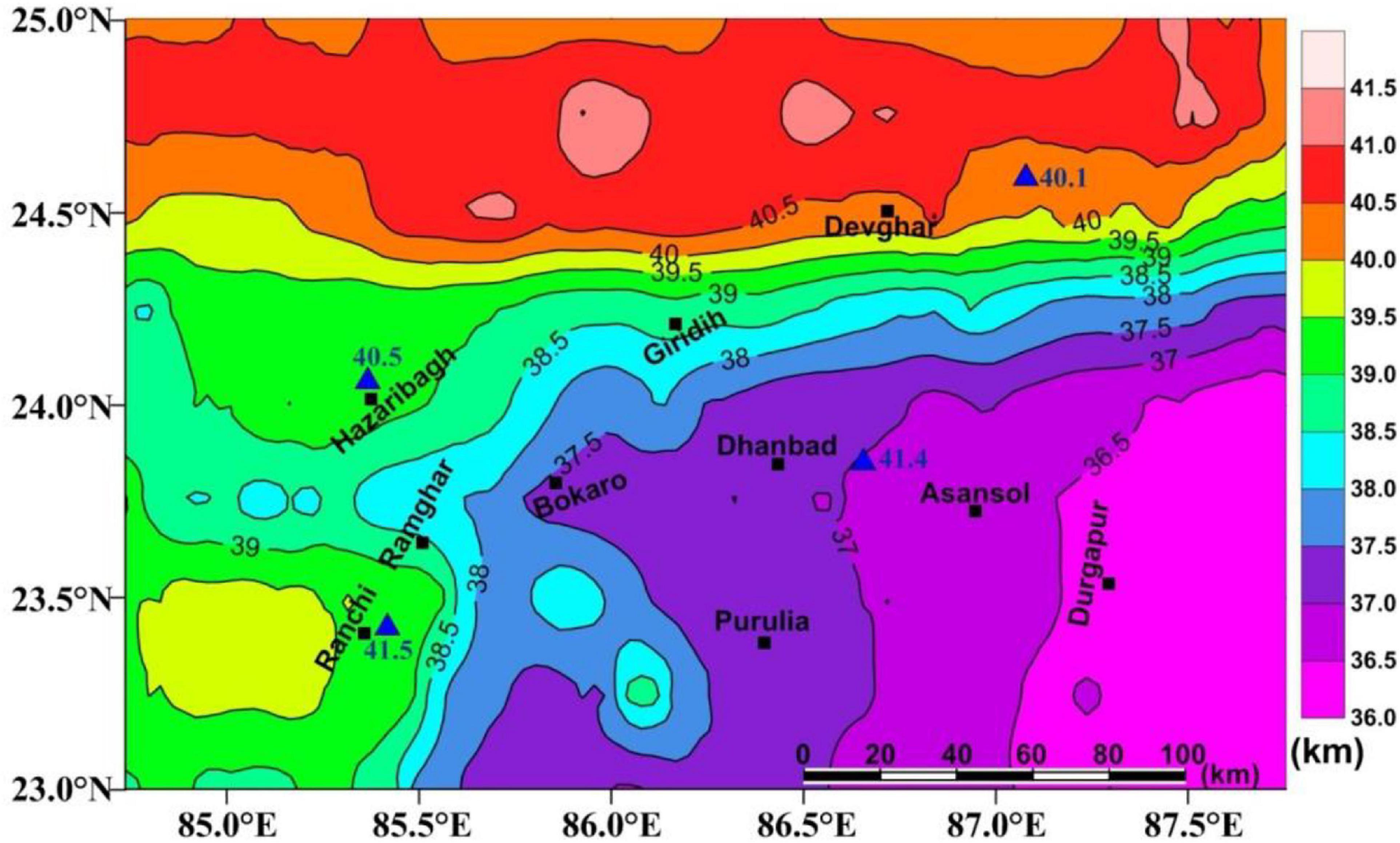
Figure 7. Moho depth map deduced from spectral analysis technique and AIRYROOT program using a contour interval of 0.5 km (with color-coded index on the east). Blue triangle represents the location of broadband seismic stations in the EIS region and below their blue color texts represent the value of Moho depth calculated by receiver function analysis (Mandal and Biswas, 2016).
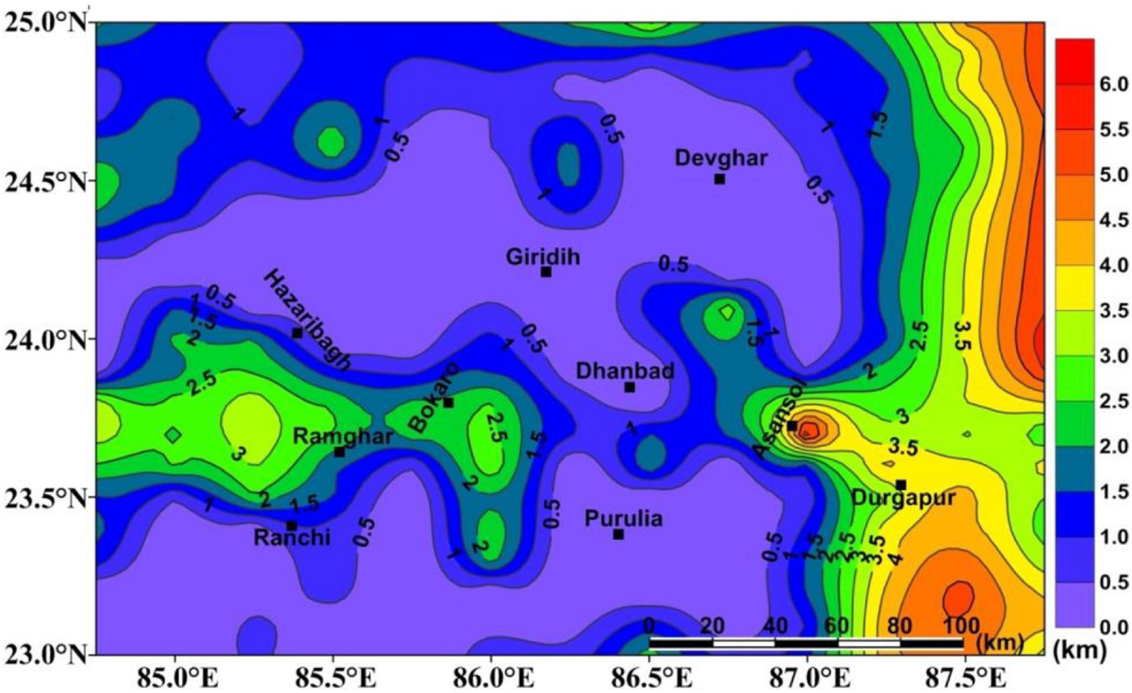
Figure 8. Sediment depth map deduced from spectral analysis, with a contour interval of 0.5 km.
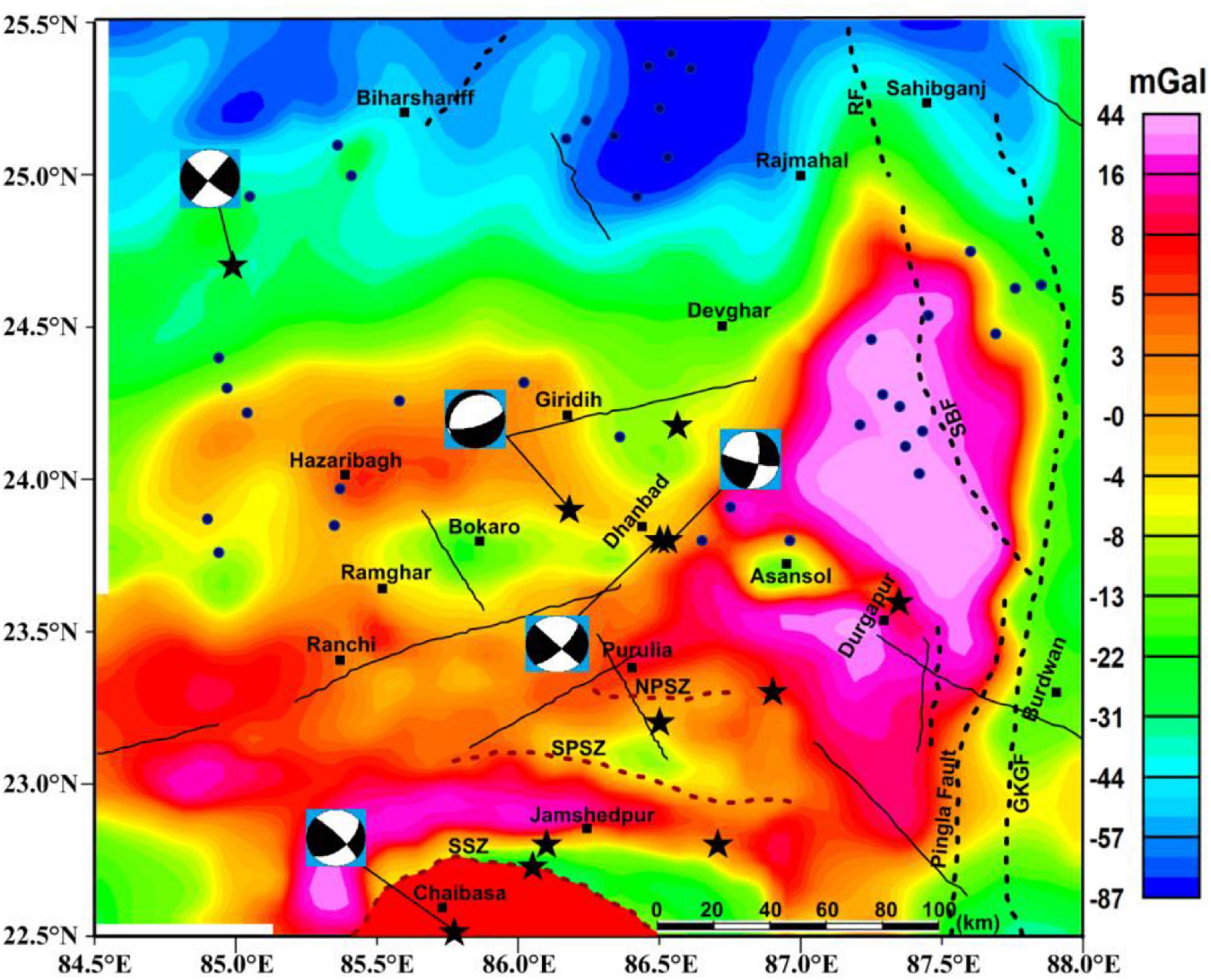
Figure 9. Airy Isostatic anomaly map of the study area, generated by removing the gravity effect of topography and its root (Airy) from the Bouguer gravity anomaly. Dark blue solid circles represent the location of the hot springs (after Sankar et al., 1991). Black stars represent the location of local earthquakes with magnitude M > 2.0, and beach balls show the focal mechanisms of some events.
The Moho depth map (Figure 7) was generated by the U.S. Geological Survey program called AIRYROOT (Simpson et al., 1983). Moho depth was also computed by 2D spectral analysis, sub-dividing the Bouguer anomaly map into 12 zones of dimension 2° × 2° (Regan and Hinze, 1976) with a uniform 75% overlap with the adjacent grid (Table 2). The sediments depth map (Figure 8) was generated by 2D spectral analysis, sub-dividing the Bouguer anomaly map into 99 zones of 1° × 1° dimension (Table 3) with a uniform 75% overlap with adjacent grid (Regan and Hinze, 1976) for better resolution and continuity of data points.
Results
Sub-surface Structures Along the Gravity Profiles
The profiles on the west (AA′ to DD′) selected over a relatively lower Bouguer gravity anomaly (Figures 6A–D), brought out six layers with some pockets of sediments. The first layer from 0 to 3.5 km comprises the Gondwana sediment with a density of 2.40–2.65 gm/cm3 and quaternary sediment of density 2.20 gm/cm3 (Choudhury, 1974). The maximum thickness found in the Damodar valley area corroborates the observation proposed by Verma (1985). The thickness of the second layer consisting of a granitic basement complex with a density of 2.67 gm/cm3 varies from 0 to ∼10 km, showing thinning toward the north. In some places, the sediments are almost absent, exposing the basement on the surface. The third layer of granite gneiss with a density of 2.71 gm/cm3 occurs from 2 to 10 km depths, thickening toward the north. The fourth layer of density 2.80 gm/cm3 is apparently a transition layer between the continental and oceanic crust. Ismaiel et al. (2019) and Krishna et al. (2019) also observed a similar layer at ∼8–13 km depth. The boundary between the lower crust (average density: 2.90 gm/cm3) and the transition layer is found at ∼17–20 km depths. The Moho depth along these profiles is found to vary between ∼38 and 40 km, corroborating the observations of Singh et al. (2015) and Mandal and Biswas (2016). Beneath the Moho, the density of the upper mantle is found to be 3.28 gm/cm3.
Profiles 5–8 (EE′ to HH′) lie over the intermediate Bouguer gravity anomaly (i.e., −80 to −15 mGal), and pass through the Bokaro-Dhanbad coal field and the Purulia shear zone. The only difference is the upper crust exposed on the surface at each profile. Here, sediment thickness is 0–2.5 km and the Moho varies from ∼37 to 41 km. The observations corroborate the observations of Verma (1985), Sharma et al. (2015), and Das et al. (2019). Profile 9 (II′) runs through the Raniganj coalfield. The deposition of the Gondwana sediments (i.e., 2.42 gm/cm3) is laterally continued from 75 to 125 km of the profile. Occasionally, the sediment is punctuated by patches of high density (2.80 gm/cm3) material. Here, Moho is found at a depth of 37–40 km, dipping toward the north. This observation is corroborated by the studies of Verma et al. (1976), Singh et al. (2015), and Mandal and Biswas (2016).
Profiles toward the east (JJ′ to MM′) pass over the relatively higher Bouguer gravity anomaly (Figures 6J–M). A total of six layers with an additional high velocity crystalline basement of density 2.75 gm/cm3 are identified along these profiles. Alluvium/sediment forming 0–4 km thick layer, with patches of Gondwana sediments, are found overlain on a 2–6 km thick layer of basement complex. A depression in the Bouguer gravity anomaly, noted at 75 km along the profile JJ′, is interpreted to be associated with ∼4–5 km basin of Gondwana sediments (density: 2.42 gm/cm3) in the Raniganj coalfield area. The profile KK′ shows a merger of ∼0.5–2 km thick Gondwana sediments with the alluvium/sediment of LGB (Verma et al., 1976). We find a high velocity layer at ∼6–8 km depth. A metasediment layer with a density of 2.65 gm/cm3 is sandwiched between the basement complex and the high velocity layer. A transition layer is identified at ∼10–12 km depth. Along profiles LL′ and MM′, a ∼3–6 km thick layer of alluvium/sediment is identified, which corroborates the observations of Qureshy (1969, 1970) and Singh et al. (2004). We have identified a fault extending from the surface to 8 km depth, at ∼80 km distance toward the south. In profile LL′, a high density (2.80 gm/cm3) material is found intruding the basement complex, but the same intruded materials are sandwiched between two sedimentary layers in the profile MM′; the high-density materials are apparently associated with the Rajmahal traps. In these areas (profiles JJ′ to MM′), Moho varies from ∼36 to 41 km.
Variation of Crustal Structure
The Moho depth (Table 4 and Figure 7) is found to vary from 40 to 41.5 km in the northern part near the IGB, apparently corroborating the observation of Singh et al. (2015), but differs from Qureshy (1969), who reported the crustal thicknesses beneath the IGB to be 37.5 km. The Damodar Gondwana basin shows moderate to low Moho depth of 37–39 km, whereas the Ranchi plateau shows a maximum depth of ∼39–40 km for the Moho; this result is well corroborated by the study of Mandal and Biswas (2016) (Table 4). The Moho depth varies from ∼37 to 37.5 km beneath the Dhanbad and Bokaro region. This observation differs from Singh et al. (2015), who found the Moho at depths between 36 and 40 km in this region. The LGB in the region of Bengal shows a minimum depth of Moho to be 36.5 km, which agrees with the Moho depth of 35–36 km computed by Singh et al. (2015). Mitra et al. (2008) found the Moho boundary at ∼37.5 km depth near the LGB. Kaila et al. (1992) also found the Moho at ∼35 km depth. We further compared the depth of Moho beneath other continents of a similar age around the world (Table 4) and found compatible results.
The map (Figure 8) illustrates that the thicknesses of sediments vary between 0.0 and 6.5 km. A strip-like region of ∼160 km lateral extent (∼23.5 to ∼24 °N) and a sediment thickness of 0.5–3.0 km is found to be associated with the Damodar Gondwana basin (Verma and Ghosh, 1977). Sediment thickness varies from 0 to 2 km toward the north near the UGB. Qureshy (1969) and Choudhury (1974) also reported similar thicknesses of the Quaternary sediments in these areas. The eastern part of the region exhibits a maximum thickness of sedimentary cover, reaching more than 6.0 km, particularly in the LGB, and corroborates the observations of Kaila et al. (1992, 1996), Mall et al. (1999), and Singh et al. (2004). At several places, on both sides of the Damodar Gondwana basin, the basement is exposed on the surface, usually found in the Achaean terrain (Verma, 1985; Veevers and Tewari, 1995; Bhattacharya and Bhattacharya, 2015; Acharyya, 2018a).
Isostatic anomaly is found to be varied from −87 to 44 mGal (Figure 9), and the minimum value is found on the northern and eastern part, where the elevation from the MSL is minimum, indicating over-compensation along the UGB. The maximum value of 44 mGal, representing the under-compensation, is identified toward the east and south near the LGB, Rajmahal trap, and Singhbhum shear zone. The coal-rich Damodar Gondwana basin (i.e., Bokaro, Dhanbad, and Asansol areas) shows −1 to −30 mGal isostatic anomalies, indicating over-compensation because of subsiding basement of the areas. The Ranchi and Hazaribagh Plateaus show almost compensated parts with values of isostatic anomalies of 0–5 mGal.
Discussion
The reconstructed map of the study area is characterized by extensively low regional gravity in the range of −40 to −10 mGal (Figure 3), with some highs in the central part in the form of oxbow-shape and the well-defined shear zones characterized by high Bouguer gravity of values around −20 mGal at the southern part. A region in the UGB, elongated from west to east between 24° and 25°N in the northern part of the study area, is characterized by relatively low Bouguer value of −50 mGal. A very low anomaly of about −80 mGal has been noted toward the northern part of this region, and might be associated with the downward flexing of the Indian basement beneath the Himalayan Foothills. The Rajmahal trap and LGB show some high Bouguer gravity, ranging between −10 and +33 mGal.
Three individual discontinuities (i.e., basement, Conrad, and Moho) show a varying sediment thickness of zero to 6.2 km with significant lateral density variation from 2.2 gm/cm3 (approximated to be alluvial sediments) to 2.40 gm/cm3 (for Gondwana sediments). The upper crustal layer with an average density of about 2.67 gm/cm3 is followed by the crystalline basement of density 2.75 gm/cm3 and transitional layer of 2.80 gm/cm3. The Conrad layer at ∼17 and 20 km is marked by a sharp increase in density of the lower crustal layer (average density is 2.90 gm/cm3). The model indicates that the crust-mantle boundary (i.e., Moho) ranges from ∼36 km in the southeastern part of the LGB to ∼42 km toward north, possibly due to the stretching and thinning of the crust toward the south. The mean density is taken as 3.28 gm/cm3 for the upper mantle layer (Table 1).
Elevation of the study area varies from zero to ∼700 m with the highest value observed at its southwest part, and the northern and eastern parts associated with the LGB show minimum elevation (Figure 1). Moho depth varies from ∼36 to 41.5 km with minimum value found in the southeast corner of the study area, near the LGB, but the northern part has a maximum depth of Moho at ∼40.5–41.5 km (Figure 7). Moho dips toward the southeast near LGB, whereas toward the north the Moho is dipping more sharply than other parts of the study area. Sediment thickness varies from 0 to 6 km beneath the study area. Maximum area shows zero sediment thickness, i.e., the basement is exposed on the surface. A few pockets of sediments are found to be associated with coal-bearing Gondwana basin. The eastern part of the study area shows a high accumulation of sediment (Figure 8).
Bouguer and Isostatic Anomalies and the Vertical Stability of the Study Area
Isostatic anomaly is the difference between the Bouguer gravity anomaly and the computed anomaly of root zone computed from the topography. Isostasy anomaly in the study area varies from −87.0 mGal to a maximum of +44.0 mGal (Figure 9). The northern part of the study area (i.e., UGB) is associated with a strong negative Bouguer anomaly (∼−55 to −96 mGal) and moderate to high negative isostatic anomaly (∼−44 to −87 mGal) with minimum elevation of topography. This apparently accounts for the over-compensation, and is presumably caused by a deficit of rock-mass in the basin (Abbas and Subramanian, 1984; Lyon-Caen and Molnar, 1985). The UGB was explained to be a down warping foredeep of the Himalayan orogen, and the sediments in this basin, subducted along with the converging Indian plate against the Eurasian plate, evolved into the Siwalik Hills, which further resulted in the flexing zone into the over-compensated area (Lyon-Caen and Molnar, 1985). Maximum positive isostatic anomaly (H-1 and H-2; +5 to +44 mGal) is observed toward the southeast near the LGB and southern part of the study area near the Singhbhum shear zone and South Purulia shear zone. Here, the low to moderate elevation of topography records little negative (∼−16 mGal) to moderate positive values (∼+33 mGal) Bouguer gravity anomalies. The positive Bouguer gravity anomaly may be due to the presence of high-density material in the shear zones, Raniganj Coal-field, and Rajmahal trap, and the positive isostatic anomaly indicates under-compensation in the region. It is clear from the sediment map that the eastern part is loaded with enormous amounts of sediments (Sengupta, 1966; Abbas and Subramanian, 1984; Alam et al., 2003; Roy and Chatterjee, 2015; Ghosh, 2018). The coal-bearing Damodar Gondwana basin accommodated the E-W extending Damodar River (Verma, 1985; Acharyya, 2018b) where the isostatic anomaly varies from ∼−22 to +5 mGal and Bouguer gravity anomaly varies from ∼−47 mGal to −24 mGal. Moderately negative Bouguer anomaly and moderately negative to slightly positive isostatic gravity anomalies account for either over-isostatic compensation or near to zero-compensation for the region. Within the drainage area, it collects huge amounts of sediments denudated from the adjacent Ranchi and Hazaribagh plateaus (i.e., under-compensated), which makes some areas over-compensated. Ranchi and Hazaribagh plateaus have a maximum elevated topography (∼700 m) and show moderate Bouguer gravity anomaly (∼−38 to −31 mGal) with little positive isostatic anomaly (+4 to +8 mGal). This apparently accounts for the little under-compensation of the area. To inquire into the overall stability, both positive and negative values of isostatic anomalies are apparent over the study area (Figure 9). Negative value within UGB corresponds to the over-compensation, reflecting higher value in Moho depth up to ∼41 to 41.5 km, whereas positive value of isostatic anomaly reflects under-compensation and less Moho depth up to 36 km in the LGB. The western part, near the Ranchi and Hazaribagh plateau, apparently falls under positive isostatic anomaly with a normal Moho depth of 39–39.5 km (Table 4). Overall, the Moho is uplifted in the southeast part, whereas it is subsided toward the north of the study area because of the down-going basement beneath the foreland Gangetic basin.
Earthquake Activities and Seismic Stability of the EIS and Adjoining Regions
The study area is tectonically very significant, comprising mainly the EIS and the Singhbhum craton, starting from the northern end of the Eastern Ghats Belt (EGB) and Bengal estuary to the bending zone beneath the IGB. A geophysical study carried out by Sengupta (1966) indicates the disappearance of the Achaean basement of the shield area below the alluvial plain of the LGB. The exposed Achaean basement in the Shillong plateau in the northeast is apparently a continuation of the Peninsular shield through the Garo-Rajmahal gap (Evans, 1964). A series of faults and fractures pass all through the western margin of the LGB (Figure 2) and are likely continued in the Himalayas toward north (Valdiya, 1976). The buried ridges of this area are likely to be isolated in the LGB in the east. A recent study (Khan et al., 2020) shows that the lithospheric deformation in the deeper part of the area is apparently active. Further, numerous hot springs in the Damodar Gondwana basin and adjacent areas near the crest of the flexural bulging of the Indian plate are facilitating reactivation of the crust through the triggering of small magnitude earthquakes because of the strain weakening processes (Mahadevan, 2002; Bilham et al., 2003).
The study area experienced a number of moderate magnitude earthquakes in the past (discussed in section “Introduction”) (Figure 2). A recent study (Singh et al., 2020) has shown that the faulting processes in the EIS are apparently dominated by strike-slip movements. It was further transformed into extension in the northeast part of the area between the junction of the Ganga and the Brahmaputra River basins. The compression tectonics dominated by thrust faulting presumably triggered many great damaging earthquakes in the Nepal-Bihar segment of the Himalayas (Figure 2). Stretching of the basement toward the northeast of the present study area is also quite active, and likely continued with the subduction of the Indian plate toward the east beneath the Myanmar microplate (Khan, 2005; Singh et al., 2020). The present earthquakes are mostly of shallow origin and low magnitude, occasionally reaching to more than 4.0 magnitude, and few occur in the lower crust (Singh et al., 2020). It is found that the depths of 20 events are very shallow (<20 km), associated with the upper crust and likely caused by reactivation processes in the basement. The role of high heterogeneities of the crust (Khan et al., 2016, 2020; Singh et al., 2019) can also be the reason for the occurrences of low to moderate magnitude earthquakes in this part of Eastern India. The recent 2011 M 6.9 Sikkim and 2015 M 7.8, 7.3 Nepal-Bihar earthquakes, and the great aftershocks of magnitudes more than 6.0, encouraged earthscientists to review the seismotectonics of the Nepal-Bihar-Sikkim segment and its southern shield areas.
Toward the southeastern side of the study area, the Indian oceanic plate is subducting below the Eurasian plate along the Andaman-Nicobar margin (Khan et al., 2020) and beneath the Myanmar microplate toward east (Khan, 2005). This has made the Bay of Bengal (BOB) seismically active with incidents of earthquakes of magnitudes (mb) 5.5, 5.7, and 5.2 in 1964, 1989, and 1992, respectively. The 1964 Midnapore earthquake was dominated by thrust-faulting (Chandra, 1977), and the other two earthquakes were dominated by strike-slip faultings (Rao et al., 2015). An analysis of earthquakes during 1900–2011 reveals that the older structural features and weak zones near the BOB and adjacent regions were reactivated by regional stress field (Murthy et al., 2010; Rao et al., 2015). The NW-SE trending fracture zones in the BOB are found to be correlated with strike-slip faultings. The seismicity in the southern and eastern parts of the BOB is dominated by thrust faulting due to a predominant N-S compression, which had back-propagated stress from the Himalayan orogen (Biswas and Majumdar, 1997).
Himalayan tectonics are likely linked with the zone of intense deformation of the oceanic lithosphere near the equatorial Indian Ocean (EIO) Basin (Geller et al., 1983; Cloetingh and Wortel, 1986). An east-west extended structural break in this area of the northern Indian Ocean is particularly associated with the diffuse segment (DeMets et al., 1990), and has isolated the Australian plate and the Indian plate in the south to southwest. The intense seismic activities, along with the occurrences of great earthquakes, operative stress fields, and the high heat flow of the area, also support this observation (Weissel et al., 1980; Geller et al., 1983; Bergman and Solomon, 1984; Weins, 1985). The ∼N-S striking aseismic 85 and 90°E ridges divide the BOB into three main sub-basins (Gopala Rao et al., 1997), apparently guiding the active stress of the lithosphere, linking the Himalayan operative tectonics through the EIS, Singhbhum craton, and the IGB. Several faults and lineaments on both sides of the Munger-Saharsa ridge are intersecting the Foothills of the Himalaya, and these geo-fractures are likely extended all through the Gangetic basin, concentrating and raising the stress in the flexing zone of the subducting Indian crust (Sibson, 1980; Marshak and Paulsen, 1997; Godin and Harris, 2014; Khan et al., 2017a; Khan et al., 2021). The plate obliquity of 0° to less than 10° of the Nepal-Bihar-Sikkim area (Khan et al., 2014) further enhances and confines the stress field around the flexing zone through interacting fractures and triggering great earthquakes by the stress build-up processes.
Conclusion
The Bouguer gravity anomaly map indicates that the study area is characterized by low (−96 mGal) to moderate (+33 mGal) regional anomalies with the maximum value over the Rajmahal trap, the LGB in the east, and over the well-defined shear zone in the south (Figure 3). The minimum Bouguer gravity anomaly values of −50 to −96 mGal are associated with the UGB, elongated along east-west between 24.5° and 25.5°N in the northern part of the study area. Such a low anomaly in the area is possibly associated with the downward flexing of the Indian basement beneath the Himalayan Foothills. Ranchi, Hazaribagh, Giridih, Bokaro, Ramgarh, and the western part of the study area are found to be associated with ∼−30 to −40 mGal anomalies. Further, a few pockets recorded low anomalies of ∼−40 to −50 mGal, as seen in Chaibasa in the extreme south. The 2D gravity modeling (Figure 5) shows a sediment layer of thicknesses of ∼0–6.5 km, with a significant density variation of 2.2–2.65 gm/cm3, underlain by a basement of a density of 2.67 gm/cm3. The Conrad is marked by an increase in density from ∼2.67 to 2.90 kg/m3 at depths between 17 and 20 km. The average density of the upper mantle layer is computed to be ∼3.28 gm/cm3. A ∼2–3 km thick high density (3.02 gm/cm3) material overlies the Moho toward the east and is apparently connected with the Rajmahal trap (Singh et al., 2004). The maximum depth of the Moho is found to be ∼40.5–41.5 km toward the north (UGB), while Moho near the LGB has the lowest depth of ∼36 km. Ranchi and Hazaribagh plateau are underlain by Moho at ∼39–39.5 km depths. The uplifted Moho and the maximum deposition of alluvium sediments are found beneath the LGB in the southeastern part (Table 4).
A residual isostatic map provides the status of stability of any study area. Based on isostatic anomaly (Figure 9), it is found that the northern part (Gangetic basin), a down-warping fore-deep of the Himalayan orogen, is over-compensated. Eastern and southern parts, comprising the LGB and shear zones (e.g., Singhbhum and North and South Purulia, Figure 1), have predominant records of under-compensation. While the coal-bearing Damodar Gondwana basin is partially over-compensated, the Ranchi and Hazaribagh plateau have achieved partial under-compensation. The present study also shows that the exposed Achaean basement of the shield area at various locations disappears below the Gangetic basin and is affected by active stretching toward the northeast of India (Singh et al., 2020). Seismic activities of this region are mostly of shallow origin, particularly associated with the basement within the upper crust. Although the region experienced a few moderate magnitude earthquakes in the historical past (Figure 2), occasional incidents of recent earthquakes have magnitudes less than 5.0. Occasional events are also found in the deeper part and might be related to the reactivation processes in the lower crust. The eastern part of the study area is also activated seismically due to the subduction processes of the Indian plate beneath the Myanmar microplate.
The long-term observations of occurrences of moderate to low magnitude earthquakes in the EIS, Singhbhum craton, and the BOB apparently account for seismic stability of the region, extending from the diffused EIO to the Nepal-Bihar-Sikkim Himalayan region. Lithospheric stress in the BOB is guided by the aseismic 85 and 90°E ridges, partially accumulated along the different fault-guided zones or other tectonic elements and triggering low-magnitude events. Sometimes, the ∼N-S striking regional fault systems (e.g., EPF, WPF, PF, MSRF, MSRMF, etc., Figure 2) also guide the stress field, concentrating and raising it in the bending zones of the downward migrating Indian lithosphere, are triggering occasional great earthquakes in the Himalaya. The back-propagation stress from the Himalayan Mountain possibly facilitates deformation in the EIO basin (Weissel et al., 1980; Geller et al., 1983; Cloetingh and Wortel, 1986; DeMets et al., 1990). The pure compression in the foothills of the Nepal Himalaya and the minimum obliquity of the converging Indian plate corroborate the observation of stress enhancement in the flexing zone of the down-going plate. We propose that the prevailing stress fields in the converging Indian lithosphere, guided by the aseismic 85 and 90°E ridges, are migrating through the low-to-moderately stable BOB and EIS. The migrating enhanced stress (because of minimum Indian plate obliquity, Figure 9 of Khan et al., 2014) is further guided by the foothill transecting fault systems to be concentrated in the bending zone of the penetrating lithosphere beneath the Himalaya. This increasing accumulated stress occasionally triggers great earthquakes in the Nepal-Bihar-Sikkim sector of the Himalaya.
Data Availability Statement
The raw data supporting the conclusions of this article will be made available by the authors, without undue reservation.
Author Contributions
All authors listed have made a substantial, direct, and intellectual contribution to the work, and approved it for publication.
Conflict of Interest
The authors declare that the research was conducted in the absence of any commercial or financial relationships that could be construed as a potential conflict of interest.
Acknowledgments
RS is thankful to the Director of the Indian Institute of Technology (ISM), Dhanbad, for financial support to complete the present work and Dhananjay Singh, Geophysicist, M & CSD, Geological Survey of India, Kolkata, West Bengal, India, for his useful and critical suggestions during the computation of 2D gravity modeling. Thanks to both of the reviewers for their valuable comments, which improved the manuscript greatly. The authors are grateful to S. P. Mohanty for thorough revision and correction and improvement of the English of the whole manuscript.
References
Abbas, N., and Subramanian, V. (1984). Erosion and sediment transport in the Ganges River basin (India). J. Hydro. 69, 173–182. doi: 10.1016/0022-1694(84)90162-8
Acharyya, S. K. (2018b). “Development of Gondwana Basins in Indian Shield,” in Tectonic Setting and Gondwana Basin Architecture in the Indian Shield, ed. S. K. Acharyya (Berlin: Elsevier), 17–29. doi: 10.1016/b978-0-12-815218-8.00003-0
Acharyya, S. K. (2018a). “Chapter 1 – Introduction,” in Tectonic Setting and Gondwana Basin Architecture in the Indian Shield, Vol. 4, ed. S. K. Acharyya (Berlin: Elsevier), 1–5. doi: 10.1016/b978-0-12-815218-8.00001-7
Alam, M., Alam, M. M., Curray, J. R., Chowdhury, M. L. R., and Gani, M. R. (2003). An overview of the sedimentary geology of the Lower Gangetic basin in relation to the regional tectonic framework and basin-fill history. Sed. Geol. 155, 179–208. doi: 10.1016/s0037-0738(02)00180-x
Altenbernd, T., Wilfried, J., and Wolfram, H. G. (2020). The bent prolongation of the 85°E Ridge south of 5°N – Fact or fiction? Tectonophysics 785:228457. doi: 10.1016/j.tecto.2020.228457
Ammon, C. J., Randall, G. E., and Zandt, G. (1990). On the non-uniqueness of receiver function inversions. J. Geophys. Res. 95, 15303–15318. doi: 10.1029/jb095ib10p15303
Ansari, M. A., Khan, P. K., Tiwari, V. M., and Banerjee, J. (2014). Gravity anomalies, flexure, and deformation of the converging Indian lithosphere in Nepal and Sikkim–Darjeeling Himalayas. Int. J. Earth Sci. 103, 1681–1697. doi: 10.1007/s00531-014-1039-0
Ates, A., and Kearey, P. (2000). Interpretation of gravity and aeromagnetic anomalies of the Kenya region, south central Turkey. J. Balkan Geophys. Soc. 3, 37–44.
Bansal, A. R., and Dimri, V. P. (2010). Scaling spectral analysis: A new tool for interpretation of gravity and magnetic data. Earth Sci. India 3, 54–68.
Bansal, A. R., Dimri, V. P., and Sagar, G. V. (2006). Depth estimation from gravity data using the maximum entropy method (MEM) and the multi taper method (MTM). Pure Appl. Geophys. 163, 1417–1434. doi: 10.1007/s00024-006-0080-8
Bergman, E. A., and Solomon, S. C. (1984). Source mechanisms of earthquakes near mid-ocean ridges from body waveform inversion: implications for the early evolution of oceanic lithosphere. J. Geophys. Res. 89, 11415–11441. doi: 10.1029/jb089ib13p11415
Bhattacharya, B. B., and Shalivahan, S. S. (2002). The electric Moho underneath Eastern Indian Craton. Geophys. Res. Lett. 29:1376.
Bhattacharya, H. N., and Bhattacharya, B. (2015). Lithofacies architecture and palaeogeography of the Late Paleozoic glaciomarine Talchir formation, Raniganj Basin, India. J. Palaeogeog. 4, 269–283. doi: 10.1016/j.jop.2015.08.006
Bhattacharyya, B. K., and Leu, L.-K. (1975). Spectral analysis of gravity and magnetic anomalies due to two dimensional structures. Geophys 40, 993–1013. doi: 10.1190/1.1440593
Bilham, R., Bendick, R., and Wallace, K. (2003). Flexure of the Indian plate and intraplate earthquakes. Proc. Indian Aca. Sci. Earth Planet. Sci. 112, 315–329. doi: 10.1007/bf02709259
Biswas, S., and Majumdar, R. K. (1997). Seismicity of the BOB: evidence for intraplate deformation of the northern Indian plate. Tectonophysics 269, 323–336. doi: 10.1016/s0040-1951(96)00168-0
Bonvalot, S., Balmino, G., Briais, A., Kuhn, M., Peyrefitte, A., Vales, N., et al. (2012). World Gravity Map. Commission for the Geological Map of the World. ed. BGI-CGMW-CNES-IRD. Paris: CGMW.
Bose, M. K. (1999). Geochemistry of the metabasics and related rocks from the eastern part of the Proterozoic Singhbhum mobile belt, eastern India—Petrogenitic implications. Indian J. Geol. 71, 213–234.
Bose, M. K. (2008). “Petrology and geochemistry of Proterozoic ‘Newer Dolerite’ and associated ultramafic dykes within Singhbhum granite pluton, eastern India,” in Indian Dykes: Geochemistry, Geophysics and Geochronology, eds. R. K. Srivastava, C. Sivaji, and N. V. Chalapathi Rao (New Delhi: Narosa Publishing House Pvt. Ltd.), 413–445.
Bose, M. K. (2009). Precambrian mafic magmatism in the Singhbhum craton, Eastern India. J. Geol. Soc. India 73, 13–135. doi: 10.1007/s12594-009-0002-3
Burdick, L. J., and Langston, C. A. (1977). Modeling crustal structure through the use of converted phases in teleseismic body-wave forms. Bull. Seismol. Soc. Am. 67, 677–691.
Carbó, A., Muñoz-Martín, A., Llanes, P., Álvarez, J., and Eez Working Group. (2003). Gravity analysis offshore the Canary Islands from a systematic survey. Mar. Geophys. Res. 24, 113–127. doi: 10.1007/1-4020-4352-x_5
Chamoli, A., and Dimri, V. P. (2010). “Spectral analysis of gravity data of NW Himalaya,” in Proceedings of the EGM 2010 International Workshop, Apr 2010, cp-165-00048, Capri.
Chamoli, A., Swaroopa Rani, V., Srivastava, K., Srinagesh, D., and Dimri, V. P. (2010). Wavelet analysis of the seismograms for tsunami warning. Nonlin. Process. Geophys. 168, 569–574. doi: 10.5194/npg-17-569-2010
Chandra, U. (1977). Earthquakes of Peninsular India–a seismotectonic study. Bull. Seismol. Soc. Am. 67, 1387–1413.
Chapin, D. (1996). A deterministic approach toward isostatic gravity residuals—a case study from South America. Geophys 61, 1022–1033. doi: 10.1190/1.1444024
Chatterjee, N., Crowley, J. L., and Ghose, N. C. (2008). Geochronology of the 1.55 Ga Bengal anorthosite and Grenvillian metamorphism in the Chhotanagpur gneissic complex, eastern India. Precambrian Res. 161, 303–316. doi: 10.1016/j.precamres.2007.09.005
Chavez, R. E., Lazaro-Mancilla, O., Campos-Enriquez, J. O., and Floresmarquez, E. L. (1999). Basement topography of the Mexicali valley from spectral and ideal body analysis of gravity data. J. South Am. Earth Sci. 12, 579–587. doi: 10.1016/s0895-9811(99)00041-3
Choudhury, S. K. (1974). Gravity and crustal thickness in the Indo-Gangetic basins and Himalayan region. India. Gcophys. J. R. Astron. Soc. 40, 441–452. doi: 10.1111/j.1365-246x.1975.tb04141.x
Cloetingh, S., and Wortel, R. (1986). Stress in the Indo-Australian plate. Tectonophysics 132, 49–67. doi: 10.1016/0040-1951(86)90024-7
Coron, S. S. (1969). “Gravity anomalies as function of elevation. Some results of Western Europe,” in The Earth’s Crust and Upper Mantle. Geophysical Monograph, 13, ed. P. J. Hart (Washington, DC: American Geophysical Union), 304–312. doi: 10.1029/gm013p0304
Curtis, C. E., and Jain, S. (1975). Determination of volcanic thickness and underlying structures from aeromagnetic maps of the Silet area of Algeria. Geophys 40, 79–90. doi: 10.1190/1.1440517
Das, M. K., Agrawal, M., Gupta, R. K., and Gautam, J. L. (2019). Lithospheric seismic structure beneath two broadband station sites of the Eastern part of Chhotanagpur plateau: new constraints from receiver functions and dispersion curves. Phys. Earth Planet. Inter. 287, 51–64. doi: 10.1016/j.pepi.2019.01.004
Dasgupta, S., Pande, P., Ganguly, D., Iqbal, Z., Sanyal, K., Venkataraman, N. V., et al. (2000). Seismotectonic Atlas of India and its Environs. Special Publication Series 59. Kolkata: Geological Survey of India, 87.
DeMets, C., Gordon, R. G., Argus, D. F., and Stein, S. (1990). Current plate motions. Geophys. J. Int. 101, 425–478. doi: 10.1111/j.1365-246x.1990.tb06579.x
DeMets, C., Gordon, R. G., Argus, D. F., and Stein, S. (1994). Effect of recent revision to the geomagnetic reversal time scale on estimates of current plate motions. Geophys. Res. Lett. 21, 2191–2194. doi: 10.1029/94gl02118
Djomani, Y. H. P., Diament, M., and Albouy, Y. (1992). Mechanical behaviour of the lithosphere beneath the Adamawa Uplift (Cameroon, West Africa) based on gravity data. J. African Earth Sci. 15, 81–90. doi: 10.1016/0899-5362(92)90009-2
Dueker, K. G., and Sheehan, A. F. (1997). Mantle discontinuity structure from midpoint stacks of converted P to S waves across the Yellowstone hotspot track. J. Geophys. Res. 102, 8313–8327. doi: 10.1029/96jb03857
Geller, G. A., Weissel, J. K., and Anderson, R. N. (1983). Heat transfer and intraplate deformation in the central Indian Ocean. J. Geophys. Res. 88, 1018–1032. doi: 10.1029/jb088ib02p01018
Geller, R. J. (1991). Supercomputers in seismology: determining 3-D earth structure. SIAM News 24:5.
Ghose, N. C. (1983). Geology, tectonics and evolution of Chotanagapur granite-gneiss complex. Eastern India. Recent Res. Geol. 10, 211–247.
Ghosh, S. C. (2018). “Nature of boundary and other faults in Raniganj Gondwana rift basin”, in Tectonic Setting and Gondwana Basin Architecture in the Indian Shield, ed. S. K. Acharyya (Amsterdam: Elsevier) 4, 33–44. doi: 10.1016/b978-0-12-815218-8.00005-4
GMSI (2006). Gravity Map Series of India (GMSI). Hyderabad: National Geophysical Research Institute and Geological Survey of India.
Godin, L., and Harris, L. B. (2014). Tracking basement cross-strike discontinuities in the Indian crust beneath the Himalayan orogen using gravity data – relationship to upper crustal faults. Geophys. J. Int. 198, 198–215. doi: 10.1093/gji/ggu131
Gomez-Ortiz, D., Tejero-Lopez, R., Babin-Vich, R., and Rivas-Ponce, A. (2005). Crustal density structure in the Spanish Central System derived from gravity data analysis (Central Spain). Tectonophysics 403, 131–149. doi: 10.1016/j.tecto.2005.04.006
Gopala Rao, D., Krishna, K. S., and Sar, D. (1997). Crustal evolution and sedimentation history of the BOB since the Cretaceous. J. Geophys. Res. 102, 17747–17768. doi: 10.1029/96jb01339
Gordon, R. G., DeMets, C., and Argus, D. F. (1990). Kinematic constraints on distributed lithospheric deformation in the equatorial Indian Ocean from present motion between the Australian and Indian plates. Tectonics 9, 409–422. doi: 10.1029/tc009i003p00409
Green, A. G. (1972). Magnetic profile analysis. Geophys. J. R. Astron. Soc. 30, 393–403. doi: 10.1111/j.1365-246x.1972.tb05823.x
Gupta, S., Mohanty, W. K., Mandal, A., and Misra, S. (2014). Ancient terrane boundaries as probable seismic hazards: a case study from the northern boundary of the Eastern Ghats Belt, India. Geosci. Fron. 5, 17–24. doi: 10.1016/j.gsf.2013.04.001
Heiskanen, W. A., and Vening Meinesz, F. A. (1958). The Earth and Its Gravity Field, Vol. 97. New York, NY: McGraw Hill Book Co. Ltd, 86–86.
Indriana, R. D. (2008). Estimasi ketebalan sedimen dan kedalaman diskontinuitas Mohorovicic daerah Jawa Timur dengan analisis power sectrum dan data anomlai gravitasi. Berkala Fisika 11, 67–74.
Ismaiel, M., Krishna, K., Srinivas, K., Mishra, J., and Saha, D. (2019). Crustal architecture and Moho topography beneath the eastern Indian and Bangladesh margins – new insights on rift evolution and continent-ocean boundary. J. Geol. Soc. 176, 553–573. doi: 10.1144/jgs2018-131
Iyer, H. M., and Hirahara, K. (1993). Seismic Tomography: Theory and Practice. Upper Saddle River, NJ: Prentice Hall.
Kaila, K. L., Murthy, P. R., MadhavaRao, N., Rao, I. B. P., Rao, P. K., Sridhar, A. R., et al. (1996). Structure of the crystalline basement in the West Lower Gangetic basin, India, as determined from deep seismic sounding studies. Geophys. J. Int. 124, 175–188. doi: 10.1111/j.1365-246x.1996.tb06362.x
Kaila, K. L., Reddy, P. R., Mall, D. M., Venkateswarlu, N., Krishna, V. G., and Prasad, A. S. S. S. R. S. (1992). Crustal structure of the West Lower Gangetic basin, India, from deep seismic sounding investigations. Geophys. J. Int. 111, 45–66. doi: 10.1111/j.1365-246x.1992.tb00554.x
Karner, G. D., and Watts, A. B. (1983). Gravity anomalies and flexure of the lithosphere at mountain ranges. J. Geophys. Res. 88, 10449–10477. doi: 10.1029/jb088ib12p10449
Kayal, J. R., Srivastava, V. K., Bhattacharya, S. N., Khan, P. K., and Chatterjee, R. (2009). Source parameters and focal mechanisms of local earthquakes: single broadband observatory at ISM Dhanbad. J. Geol. Soc. India 4, 413–419. doi: 10.1007/s12594-009-0144-3
Kayal, J. R., Srivastava, V. K., Kumar, P., Chatterjee, R., and Khan, P. K. (2011). Evolution of crustal 869 and upper mantle structures using receiver function analysis: ISM broad band 870 observatory data. J. Geol. Soc. India 78, 76–80. doi: 10.1007/s12594-011-0069-5
Khan, P. K. (2005). Variation in dip-angle of the Indian plate subducting beneath the Burma plate and its tectonic implications. Geosci. J. 9, 227–234. doi: 10.1007/bf02910582
Khan, P. K., Ansari, A., and Singh, D. (2017a). Insights into the great Mw 7.9 Nepal earthquake of 25 April 2015. Curr. Sci. 113, 2014–2020. doi: 10.18520/cs/v113/i10/2014-2020
Khan, P. K., Ansari, M. A., and Mohanty, S. (2014). Earthquake source characteristics along the arcuate Himalayan belt: geodynamic implications. J. Earth Sys. Sci. 123, 1013–1030. doi: 10.1007/s12040-014-0456-6
Khan, P. K., Bhukta, K., and Mandal, P. (2020). Estimation of source parameters of local earthquakes based on inversion of waveform data. Curr. Sci. 119:7.
Khan, P. K., Mohanty, S. P., Chakraborty, P. P., and Singh, R. (2021). Earthquake shocks around Delhi-NCR and the adjoining himalayan front: a seismotectonic perspective. Front. Earth Sci. 9:598784. doi: 10.3389/feart.2021.598784
Khan, P. K., Shamim, Sk, Mohanty, M., Kumar, P., and Banerjee, J. (2017b). Myanmar-Andaman-Sumatra subduction margin revisited: insights of arc-specific deformations. J. Earth Syst. Sci. 28, 683–694. doi: 10.1007/s12583-017-0752-6
Kosarev, G. L., Oreshin, S. I., Vinnik, L. P., Kiselev, S. G., Dattatrayam, R. S., Suresh, G., et al. (2013). Heterogeneous lithosphere and the underlying mantle of the Indian subcontinent. Tectonophysics 592, 175–186. doi: 10.1016/j.tecto.2013.02.023
Krishna, K. S., Ismaiel, M., Srinivas, K., and Saha, D. (2019). Ancient ocean floor hidden beneath Bangladesh. Curr. Sci. 117, 916–917.
Kumar, M. R., Saul, J., Sarkar, D., Kind, R., and Shukla, A. (2001). Crustal structure of the Indian shield; new constraints from teleseismic receiver functions. Geophys. Res. Lett. 28, 1339–1342. doi: 10.1029/2000gl012310
Kumar, N., Singh, A. P., and Tiwari, V. M. (2020). Gravity anomalies, isostasy and density structure of the Indian Continental Lithosphere. Episod 43, 609–621. doi: 10.18814/epiiugs/2020/020040
Kumar, P., Kumar, M. R., Srijayanthi, G., Arora, K., Srinagesh, D., Chadha, R. K., et al. (2013). Imaging the lithosphere-asthenosphere boundary of the Indian plate using converted wave technique. J. Geophys. Res. 118, 5307–5319. doi: 10.1002/jgrb.50366
Lefort, J. P., and Agarwal, B. N. P. (2002). Topography of the Moho undulations in France from gravity data: their age and origin. Tectonophysics 350, 193–213. doi: 10.1016/s0040-1951(02)00114-2
Lyon-Caen, H., and Molnar, P. (1985). Gravity anomalies, flexure of the Indian plate, and the structure, support and evolution of the Himalaya and Ganga Basin. Tectonics 4, 513–538. doi: 10.1029/tc004i006p00513
Lyons, S. N., Sandwell, D. T., and Smith, W. H. F. (2000). Three-dimensional estimation of elastic thickness under the Louisville ridge. J. Geophys. Res. 105:252.
Mall, D. M., Rao, V. K., and Reddy, P. R. (1999). Deep sub-crustal features in the Lower Gangetic basin: Seismic signatures for plume activity. Geophys. Res. Lett. 26, 2545–2548. doi: 10.1029/1999gl900552
Mandal, P., and Biswas, K. (2016). Teleseismic receiver functions modeling of the eastern Indian craton. Phys. Earth Planet. Inter. 258, 1–14. doi: 10.1016/j.pepi.2016.07.002
Marshak, S., and Paulsen, T. (1997). Structural style, regional distribution, and seismic implications of midcontinent fault-and-fold zones, United States. Seismol. Res. Lett. 68, 511–520. doi: 10.1785/gssrl.68.4.511
Maus, S., and Dimri, V. P. (1995). Potential field power spectrum inversion for scaling geology. J. Geophys. Res. 100, 12605–12616. doi: 10.1029/95jb00758
McKenzie, D., and Sclater, J. G. (1971). The evolution of the Indian Ocean since the Late Cretaceous. Geophys. J. Int. 24, 437–528. doi: 10.1111/j.1365-246x.1971.tb02190.x
Minster, J. B., and Jordan, T. H. (1978). Present-day plate motions. J. Geophys. Res. 83, 5331–5354. doi: 10.1029/jb083ib11p05331
Mishra, D. C., Laxman, G., and Arora, K. (2004). Large-wavelength gravity anomalies over the Indian continent: indicators of lithospheric flexure and uplift and subsidence of Indian peninsular shield related to isostasy. Curr. Sci. 86, 861–867.
Mitra, S., Bhattacharya, S. N., and Nath, S. K. (2008). Crustal structure of the Western Lower Gangetic basin from joint analysis of teleseismic receiver functions and Rayleigh wave dispersion. Bull. Seismol. Soc. Am. 98, 2715–2723. doi: 10.1785/0120080141
Murthy, K. S. R., Subrahmanyam, V., Subrahmanyam, A. S., Murty, G. P. S., and Sarma, K. V. L. N. S. (2010). Land-ocean tectonics (LOTs) and the associated seismic hazard over the Eastern continental margin of India (ECMI). Nat. Hazards 55, 167–175. doi: 10.1007/s11069-010-9523-8
Naqvi, S. M., and Rogers, J. J. W. (1987). Precambrian Geology of India. New York, NY: Oxford University Press Inc, 223.
Odegard, M. E., and Berg, J. W. (1965). Gravity interpretation using the Fourier integral. Geophys 33, 424–438. doi: 10.1190/1.1439598
Pandey, A. C., Kumar, A., and Jeyaseelan, A. T. (2013). Urban built-up area assessment of Ranchi Township using Cartosat-I stereopairs satellite images. J. Indian Soc. Remote Sens. 41, 141–155. doi: 10.1007/s12524-012-0209-4
Pandey, O. P., and Agarwal, P. K. (1999). Lihtospheric mantle deformation beneath the Indian cratons. J. Geol. 107, 683–692. doi: 10.1086/314373
Parker, R. L. (1972). The rapid calculation of potential anomalies. Geophys. J. R. Astron. Soc. 31, 447–455. doi: 10.1111/j.1365-246x.1973.tb06513.x
Pick, M., Picha, J., and Vyskocil, V. (1973). Theory of the Earth’s Gravity Field. Prague: Academia.
Prasanna, H. M. I., Chen, W., and İz, H. B. (2013). High resolution local Moho determination using gravity inversion: a case study in Sri Lanka. J. Asian Earth. Sci. 74, 62–70. doi: 10.1016/j.jseaes.2013.06.005
Qureshy, M. N. (1969). Thickening of a basalt layer as a possible cause for the uplift of the Himalayas-A suggestion based on gravity data. Tectonophysics 7, 137–157. doi: 10.1016/0040-1951(69)90003-1
Qureshy, M. N. (1970). “Relation of gravity to elevation, geology and tectonics of India,” in Proceedings of the II UMP Symp, Hyderabad, 1–23. doi: 10.1007/978-3-642-96785-6_1
Qureshy, M. N. (1981). Gravity anomalies, isostasy and crust-mantle relations in the Deccan Trap and contiguous regions. India. Geol. Soc. India Mem. 3, 184–197.
Qureshy, M. N., and Warsi, W. E. K. (1980). A Bouguer anomaly map of India and its relation to broad tectonic elements of the subcontinent. Geophy. J. Roy. Astron. Soc. 61, 235–242. doi: 10.1111/j.1365-246x.1980.tb04314.x
Rao, G. S., Radhakrishna, M., and Murthy, K. S. R. (2015). A seismotectonic study of the 21 May 2014 BOB intraplate earthquake: evidence of onshore-offshore tectonic linkage and fracture zone reactivation in the northern BOB. Nat. Hazards 78, 895–913. doi: 10.1007/s11069-015-1750-6
Rastogi, B. K. (2016). Seismicity of Indian Stable continental region, 2016. J. Earthquake. Sci. Eng. 3, 57–93.
Regan, R. D., and Hinze, W. J. (1976). The effect of finite data length in the spectral analysis of ideal gravity anomalies. Geophys 41, 44–55. doi: 10.1190/1.1440606
Reguzzoni, M., Sampietro, D., and Sanso, F. (2013). Global Moho from the combination of the CRUST2.0 model and GOCE data. Geophys. J. Int. 195, 222–237. doi: 10.1093/gji/ggt247
Riad, S., and El-Etr, H. A. (1985). Bouguer anomalies and lithosphere-crustal thickness in Uganda. J. Geodyn. 3, 169–186. doi: 10.1016/0264-3707(85)90027-4
Riad, S., Fouad, A., Refai, E., and Ghalib, M. (1983). “Preliminary interpretation of regional gravity anomalies of Egypt,” in Proceedings of the IUGG Inter-disciplinary Symposium Hamburg, Hamburg.
Rivero, L., Pinto, V., and Casas, A. (2002). Moho depth structure of the eastern part of the Pyrenean belt derived from gravity data. J. Geodyn. 33, 315–332. doi: 10.1016/s0264-3707(01)00073-4
Roy, A. B., and Chatterjee, A. (2015). Tectonic framework and evolutionary history of the Lower Gangetic basin in the Indian subcontinent. Curr. Sci. 109, 271–279.
Sankar, R., Guha, S. K., Seth, N. N., Muthuraman, K., Pitale, U. L., Jangi, B. L., et al. (1991). Geothermal Atlas of India. Geol. Sur. India 19:144.
Sarkar, A. N. (1982). Precambrian tectonic evaluation of eastern India: a model of converging microplates. Tectonophysics 86, 363–397. doi: 10.1016/0040-1951(82)90180-9
Sarkar, S. N., and Saha, A. K. (1977). Present status of the Precambrian stratigraphy, tectonics and geochronology of Singhbhum, Keonjhar, Mayurbhanj region, Eastern India. Indian J. Earth Sci. 4, 37–55.
Sastri, V. V., Bhandari, L. L., Raju, A. T. R., and Datta, A. K. (1971). Tectonic framework and subsurface stratigraphy of the Ganga basin. J. Geol. Soc. India 12, 222–233.
Sengupta, S. (1966). Geological and geophysical studies in western part of Lower Gangetic basin, India. Am. Assoc. Petrol. Geolog. Bull. 50, 1001–1017.
Sharma, N. K., Khan, P. K., and Bhukta, K. K. (2015). Nature of the Moho in the mid-eastern part of the Chhotanagpur Plateau, India, from a receiver function perspective. Arabian J. Geosci. 8, 5669–5675. doi: 10.1007/s12517-014-1648-8
Shin, Y. H., Xu, H., Braitenberg, C., Fang, J., and Wang, Y. M. (2007). Moho undulations beneath Tibet from GRACE-integrated gravity data. Geophy. J. Int. 170, 971–985. doi: 10.1111/j.1365-246x.2007.03457.x
Sibson, R. H. (1980). Transient discontinuities in ductile shear zones. J. Struct. Geol. 2, 165–171. doi: 10.1016/0191-8141(80)90047-4
Simpson, R. W., Jachens, R. C., and Blakely, R. J. (1983). AIRYROOT: A FORTRAN program for calculating the gravitational attraction of an Airy isostatic root out to 166.7 km. U.S. Geol. Surv. Open File Rep. 8:66.
Simpson, R. W., Jachens, R. C., and Blakely, R. J. (1986). A New Isostatic Residual Gravity Map of the conterminous United States with a Discussion on the Significance of Isostatic Residual Anomalies. J. Geophys. Res. 91, 8348–8372. doi: 10.1029/jb091ib08p08348
Singh, A. P., Kumar, N., and Singh, B. (2004). Magmatic underplating beneath the Rajmahal traps: gravity signatures and derived 3-D configuration. Proc. Indian Acad. Sci. 113, 759–769. doi: 10.1007/bf02704035
Singh, A. P., Kumar, N., and Zeyen, H. (2015). Three-dimensional lithospheric mapping of the EIS: A multi-parametric inversion approach. Tectonophysics 665, 164–176. doi: 10.1016/j.tecto.2015.09.038
Singh, R., Khan, P. K., and Singh, A. P. (2020). Earthquake source dynamics and kinematics of the EIS and adjoining regions. Acta Geophys. 68, 337–355. doi: 10.1007/s11600-020-00418-z
Singh, R., Sharma, S., Mitra, S., and Khan, P. K. (2019). Mapping of coda-wave attenuation and its frequency dependency Over EIS. Pure Appl. Geophys. 176, 5291–5313. doi: 10.1007/s00024-019-02284-3
Song, P., Zhang, X., Liu, Y., and Teng, J. (2017). Moho imaging based on receiver function analysis with teleseismic wavefield reconstruction: application to South China. Tectonophysics 718, 118–131. doi: 10.1016/j.tecto.2017.05.031
Spector, A., and Grant, F. S. (1970). Statistical models for interpreting aeromagnetic data. Geophys. 35, 293–302. doi: 10.1190/1.1440092
Stein, S., and Okal, E. A. (1978). Seismicity and tectonics of the Ninetyeast Ridge area: Evidence for internal deformation of the Indian plate. J. Geophys. Res. 83, 2233–2245. doi: 10.1029/jb083ib05p02233
Tealeb, A., and Riad, S. (1986). “Regional gravity anomalies of western Saudi Arabia and their geological significance,” in Proceedings of the 5 Ann. The Meeting of E. G. S, Cairo, 50–89. doi: 10.4324/9781003074601-3
Thompson, D. A., Bastow, I. D., Helffrich, G., Kendall, J. M., Wookey, J., Snyder, D. B., et al. (2010). Precambrian crustal evolution: seismic constraints from the Canadian Shield, Earth Planet. Sci. Lett. 297, 655–666. doi: 10.1016/j.epsl.2010.07.021
Tiwari, V. M. (2003). Analysis of satellite gravity and bathymetry data over Ninety-East Ridge: variation in the compensation mechanism and implication for emplacement process. J. Geophy. Res. 108, ETG 13-1-16. doi: 10.1029/2000JB000047
Tselentis, G. A., Drakopoulos, J., and Dimitriadis, K. (1988). A spectral approach to Moho depths estimation from gravity measurements in Epirus (NW Greece). J. Phys. Earth 36, 255–266. doi: 10.4294/jpe1952.36.255
Tsuboi, C. (1979). Gravity. Crows Nest: George Allen & Unwin (Publishers) Ltd. (1983 English translation).
Tugume, F., Nyblade, A., Julià, J., and van der Meijde, M. (2013). Precambrian crustal structure in Africa and Arabia: Evidence lacking for secular variation. Tectonophysics 609, 250–266. doi: 10.1016/j.tecto.2013.04.027
Valdiya, K. S. (1976). Himalaya transverse faults and their parallelism with subsurface structures of North Indian planes. Tectonophysics 32, 353–386. doi: 10.1016/0040-1951(76)90069-x
Valdiya, K. S., and Sanwal, J. (2017). “The dynamic Indian crust,” in Neotectonism in the Indian Subcontinent - Landscape Evolution, (Amsterdam: Elsevier), 458. doi: 10.1016/b978-0-444-63971-4.00001-3
Veevers, J. J., and Tewari, R. C. (1995). Gondwana Master Basin of Peninsular India between Tethys and the Interior of the Gondwanaland Province of Pangea. GSA Mem. 187, 1–73.
Verma, R. K. (1985). “Gravity field and tectonics of Gondwana basins of Peninsular India,” in Gravity Field, Seismicity and Tectonics of the Indian Peninsula and the Himalayas (Solid Earth Sciences Library), Vol. 3, ed. R. K. Verma (Dordrecht: Springer), 44–60.
Verma, R. K., Bandyopadhyay, T. K., and Mukhopadhyay, M. (1980). Gravity field, structure and tectonics of the Raniganj coalfield three dimensional model. J. Geol. Soc. India 21, 117–127.
Verma, R. K., and Ghosh, D. (1977). “Gravity field, structure and tectonics of some Gondwana basins of Damodar valley India,” in Geophysical Case Histories of India, Vol. 1, ed. V. L. S. Bhimsamkasam (Hyderabad: AEG), 97–112.
Verma, R. K., Majumdar, R., Ghosh, D., Ghosh, A., and Gupta, N. C. (1976). Results of gravity survey over Raniganj Coalfield. India. Geophys. Prosp. 24, 19–30. doi: 10.1111/j.1365-2478.1976.tb00382.x
Watts, A. B., Bodine, J. H., and Ribe, N. M. (1980). Observations of flexure and geological evolution of the Pacific Ocean basin. Nature 283, 532–537. doi: 10.1038/283532a0
Weaver, B. L. (1990). “Early Precambrian basic rocks of India,” in Early Precambrian Basic Magmatism, eds R. P. Hall and D. J. Hughes (Glasgow: Blackie), 339–351. doi: 10.1007/978-94-009-0399-9_15
Weins, D. A. (1985). Historical seismicity near Chagos: a complex deformation zone in the equatorial Indian Ocean. Earth Planet. Sci. Lett. 76, 350–360. doi: 10.1016/0012-821x(86)90086-5
Weissel, J. K., Andreson, R. N., and Geller, C. A. (1980). Deformation of the Indo–Australian plate. Nature 287, 284–291. doi: 10.1038/287284a0
Woollard, G. P. (1969) “Regional variations in gravity. The earth’s crust and upper mantle,”in Geophysical Monograph Series, Vol. 13, (National Academy of Sciences-National Research Council Publication 1708), ed. P. J. Hart, (Washington, DC: AGU), 320–341.
Zhao, D., Hasegawa, A., and Horiuchi, S. (1992). Tomographic Imaging of P and S wave velocity structure beneath northeast Japan. J. Geophys. Res. 97:928.
Zhu, L. P. (2000). Crustal structure across the San Andreas fault, southern California from teleseismic converted waves. Earth Planet. Sci. Lett. 179, 183–190. doi: 10.1016/s0012-821x(00)00101-1
Keywords: gravity modeling, spectral analysis, crustal discontinuity, Eastern Indian Shield, isostasy
Citation: Singh R and Khan PK (2021) Crustal Configuration and Seismic Stability of the Eastern Indian Shield and Adjoining Regions: Insights for Incidents of Great Earthquakes in the Nepal-Bihar-Sikkim Himalaya. Front. Earth Sci. 9:586152. doi: 10.3389/feart.2021.586152
Received: 22 July 2020; Accepted: 09 March 2021;
Published: 31 March 2021.
Edited by:
Sebastiano D’Amico, University of Malta, MaltaReviewed by:
Santanu Baruah, North East Institute of Science and Technology (CSIR), IndiaDaniele Spatola, University of Malta, Malta
Copyright © 2021 Singh and Khan. This is an open-access article distributed under the terms of the Creative Commons Attribution License (CC BY). The use, distribution or reproduction in other forums is permitted, provided the original author(s) and the copyright owner(s) are credited and that the original publication in this journal is cited, in accordance with accepted academic practice. No use, distribution or reproduction is permitted which does not comply with these terms.
*Correspondence: Prosanta Kumar Khan, a2hhbnByb3NhbnRhMTk2NkBpaXRpc20uYWMuaW4=; a2hhbnByb3NhbnRhMTk2NkBnbWFpbC5jb20=