Multiband Wavelet Age Modeling for a ∼293 m (∼600 kyr) Sediment Core From Chew Bahir Basin, Southern Ethiopian Rift

Introduction

When investigating paleoclimate records derived from lake cores, the reliability of the age model used is crucial. This reliability depends largely on the density of independent age-control points, which should ideally be evenly distributed along the entire length of the core. Such age-control points are derived from radiometric age determinations obtained by, for example, 40Ar/39Ar dating of volcanic ash layers, 14C dating of organic material, or luminescence dating of feldspar and quartz crystals. Datable material is, however, often scarce in sediment cores. Cyclostratigraphy can be used in such cases to add additional age control points, evenly distributed in time. This method has been applied since the mid-1970s to marine records that extend beyond the range of the radiocarbon dating technique (e.g., Hays et al., 1976; Imbrie and Imbrie, 1980; Pisias et al., 1984; Martinson et al., 1987; Tiedemann et al., 1994; Grant et al., 2017). Orbital tuning has often been used to increase the temporal resolution between radiometric age control points, more commonly in paleoceanography than in paleolimnology (e.g., Grant et al., 2017).

Traditional tuning techniques first assume a maximum age for the base of the core (the base age), which is typically derived from existing radiometric dating and/or magnetostratigraphy, to derive a preliminary linear age model assuming constant sedimentation rates. (e.g., Hays et al., 1976; Pisias et al., 1984; Martinson et al., 1987; Tiedemann et al., 1994). The next step involves using a bandpass filter to reduce the proxy data to a single orbital frequency, which should match that of the tuning target (TT). The TT is a reference time series used during tuning, whose exact time course is known and whose frequency is also expressed in the proxy data. The final step is then to align the peaks of the filtered time series with those of the TT (fine tuning the preliminary age model) and to interpolate all core data to the new tuned age model.

Variants of this technique use frequency shifts by applying a moving-window Fourier technique Meyers et al., 2001), a method that tracks the dominant harmonic in the data series (Park and Herbert, 1987), an average spectral misfit method (Meyers and Sageman, 2007), a method that identifies the time scale that simultaneously optimizes eccentricity amplitude modulation of the precession band (Meyers, 2015), or a spectral moment approach (Sinnesael et al., 2018), to establish an age model (Hinnov, 2013, and references therein). Some published applications of the method have been criticized for over tuning (e.g. Tiedemann et al., 1994; Raymo et al., 1997) which is why Muller and MacDonald (2002) proposed the use of minimal tuning, for which only a few age control points are required (for example ages obtained from magnetic field reversals or radiometric ages) obtained from within the core. One of the main assumptions of the minimal tuning methods is a relatively constant sedimentation rate, which allows a stationary bandpass filter to be used. This tuning method, which is increasingly popular in paleolimnology (e.g., Wagner et al., 2019), consequently needs to be adapted in order to be applicable to lake environments, where the sedimentation rate is unlikely to be constant.

In this paper we present a new tuning technique that is suitable for use with paleoclimate records that have few radiometric age determinations but show significant orbital cyclicity. The fundamental difference between this new technique and other tuning techniques is that instead of a fixed bandpass filter we use a new adaptive filtering method that takes into account continuous long-term changes in sedimentation rates. The multiband wavelet age modeling (MUBAWA) approach uses a continuous wavelet spectral analysis to identify and trace the orbital signal within a user-defined range of possible base ages for the core.

We first used a synthetic example to demonstrate the advantages of the new method compared to a traditional method of cyclostratigraphy similar to the minimal tuning approach of Muller and MacDonald (2002). We then applied the technique to a 292.87 m composite core collected from the Chew Bahir basin in southern Ethiopia. The results demonstrate how this method can be used to further improve orbital tuning as an age-modeling technique and facilitate its use in a broad range of applications.

Methods

The Principle of the MUBAWA Approach

The MUBAWA approach is based on the application of a continuous wavelet transformation (CWT) to a depth series, with the aim of generating a tuned age model. We use the CWT to track variations in the spatial frequency of the astronomical component with depth (which we refer to as the spatial frequency path), in order to be able to adaptively bandpass filter the astronomical component from the proxy data. The MUBAWA technique is specifically designed for lacustrine depositional environments such as that of the Chew Bahir basin, with their continuous, long-term changes in sedimentation rates, whereas methods using stationary filters are not suitable for such complex depositional environments.

The MUBAWA algorithm consists of several modular functions, which are wrapped in a MATLAB live script and are available in the Supplementary material. The algorithm is divided into the following four steps (Figure 1). Step 1: preprocessing, which involves resampling and evenly spacing the input data defined by the frequency of the TT and the maximum possible base age (tmax). Step 2: spatial frequency range approximation (SFRA), which is an optional step that uses the available age control to approximate the spatial frequency range of the targeted orbital component, Step 3: spatial frequency path mapping, which involves determining spatial frequencies using a CWT and applying a weighting function to prevent the inclusion of unrealistic sedimentation rates, and Step 4: identification of the best continuous spatial frequency path, adaptive filtering by the consecutive application of Taner filters along this spatial frequency path, and identification of the best age model solution.

FIGURE 1

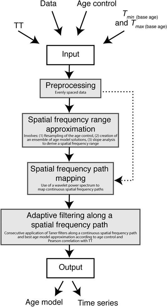
FIGURE 1. Flow chart of the multiband wavelet age modeling algorithm, showing the individual steps involved in the analysis. Gray boxes represent MATLAB functions provided in the supplementaries. Please note that the spatial frequency range approximation step can be skipped, as indicated by the bypass arrow.

Preprocessing

The filter methods used in this method, as well as the CWT, require evenly spaced data and the sample size should be restricted in order to avoid long computation times. We chose a sample size that did not exceed 20 data points for each cycle occurring in the TT within the time interval between t₀ and t_max. We then established an evenly spaced depth vector to match the new sampling rate and interpolated the proxy values in order to obtain an evenly spaced subsampled data set. The resulting computed depth series was then used in all of the subsequent steps.

Spatial Frequency Range Approximation (SFRA)

In this step we use the age control points and their corresponding uncertainties to estimate a spatial frequency range, which is defined by the frequency of the TT and the maximum and minimum slopes of the ensemble of age model solutions for each depth point. This procedure is based on the assumption that every age model solution results in a particular spatial frequency path for each depth point, depending on the frequency of the TT and the slope of the age model solution. This procedure can help to find tuned age model solutions that conform with the age control points (within their respective uncertainties). This is an optional procedure that is not essential for the determination of a frequency path, but it provides an auxiliary strategy with which to improve the chances of approximating a path that will yield results that conform with the age control points, within their uncertainty ranges.

This resampling-based approach involves obtaining random samples from the normal distribution of the available age control points and computing an age model for each set of random samples. A piecewise cubic Hermite interpolating polynomial (PCHIP; Fritsch and Carlson, 1980) is used to interpolate between the resampled age control points. Using a PCHIP yields solutions that tend not to have any strong fluctuations, since the interpolations are generally more gradual and do not deviate markedly from each other in the way that they do with other methods, such as the classic cubic spline interpolation method.

The maximum and minimum slopes of the age models derived from the resampling of the age control points, are then computed for each depth point. Only monotonically increasing solutions are accepted, in order to avoid any solutions that describe time reversals. The slopes are converted into a spatial frequency range with respect to the TT. Two depth series are then generated in which the maximum slope values lead to a depth series with a low spatial frequency limit, and the minimum slope values to a depth series with a high spatial frequency limit.

The spatial frequency limits are then used to adaptively bandpass filter the regularly sampled depth series obtained from the preprocessing, using Taner filters (Taner 1992).

Spatial Frequency Path Mapping

The following steps use either the adaptively filtered depth series obtained from the SFRA or, if the SFRA has not been used, the preprocessed depth data.

A continuous power spectrum (CWT) resolves the evolution of frequencies through time or space. Throughout this paper we focus on the perspective of spatial frequencies, since we are dealing with depth series. A spatial frequency path can be obtained by analyzing the frequency evolution of a CWT-based wavelet power spectrum of the input depth series. Further on in this section, we describe how we identify these paths. We then use the identified spatial frequency paths to adjust bandpass filter center points for each point in the depth series, thus creating an adaptive filter.

A wavelet is the basis function used for the wavelet transformation (WT) and can be thought of a specific wave defined by its frequency and amplitude, with the amplitude decaying to zero toward either end. Since wavelets can be stretched and translated in both frequency and space, with a flexible resolution, they can easily map changes in the spatial frequency domain (Figures 2A,B). We define $\beta$ as the depth variable such that $y\left(\beta \right)$ is the signal under consideration (i.e. the climate proxy data as a function of the core depth $\beta$). A continuous wavelet transformation (CWT) mathematically decomposes $y\left(\beta \right)$ into the elementary functions ${\Psi }_{a,b}\left(\beta \right)$, derived from a mother wavelet $\Psi \left(\beta \right)$ by dilation and translation (Addison, 2017). The dilation indicates a compressing or stretching of the mother wavelet $\Psi \left(\beta \right)$, resulting in a variation in its frequency, controlled by the scale parameter a. The spatial resolution of the CWT follows the translation of the mother wavelet $\Psi \left(\beta \right)$ along the depth $\beta$ and is controlled by the translation parameter b (Lau and Weng, 1995). The wavelet transform of the signal $y\left(\beta \right)$ is then defined as the convolution integral

${\text{CWT}}_{\Psi }\left(a,b\right)=\frac{1}{\sqrt{a}}{{\displaystyle {\displaystyle \int {\Psi }^{\ast }\left(\frac{\beta -b}{a}\right)y\left(\beta \right)d\beta }}}^{\text{}}(1)$

in which the asterisk indicates the complex conjugate of the mother wavelet $\Psi$ and the factor $1/\sqrt{a}$ ensures the preservation of energy. By varying b for a range of values for the scale parameter a, the final wavelet power spectrum and the corresponding scalogram can be obtained (Equation 4; Figure 2B).

FIGURE 2

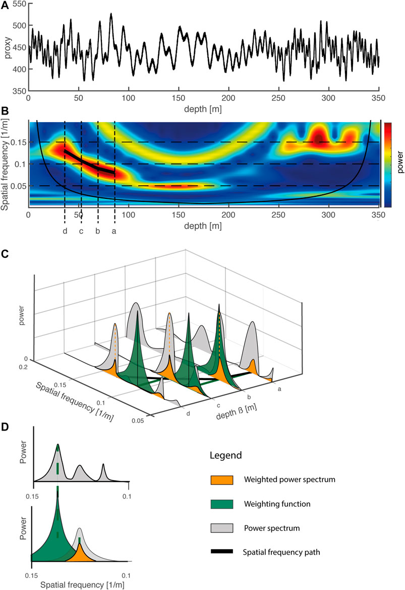
FIGURE 2. (A) To illustrate how to map spatial frequency paths we generated a demonstration depth series consisting of an insolation signal (from Laskar et al., 2004) and superimposed sinusoids. The result was a depth series that had been stretched and compressed by variations in the sedimentation rate. (B) We computed a CWT from the depth series and plotted the results in a wavelet power spectrum. Note that the frequency evolution followed curved paths. We extracted four profiles from the CWT, labeled a, b, c, and d. (C) Showing how continuous spatial frequency paths are mapped along the profiles a, b, c, and d. (D) Showing how a peak is detected and how the power spectrum of the next profile is weighted by application of the green weighting function. The gray peak is weighted and forms the orange weighted power spectrum.

The CWT can be computed for a broad spectrum of different mother wavelets. In geoscience, however, the complex Morlet wavelets are most widely used because they can be more easily adapted to capture oscillatory behavior (Torrence and Compo, 1998):

${\Psi }_{\text{Morlet}}\left(\beta \right)=\frac{1}{{\pi }^{1/4}}{e}^{i2\pi f_0\beta }{e}^{-{\beta }^2/2}(2)$

from which the elementary functions

${\Psi }_{a,b}\left(\beta \right)=\frac{1}{{\pi }^{1/4}}{e}^{\left(i2\pi f_0\frac{\beta -b}{a}\right)}{e}^{-{\left(\frac{\beta -b}{\sqrt{2}a}\right)}^2}(3)$

are derived and then used in Equation 1. Computing the CWT of the spatial data results in a complex spatial frequency output, of which the absolute value represents a wavelet power spectrum for a particular (a,b)-parameter configuration:

$E\left(a,b\right)={\left|\text{CWT}\left(a,b\right)\right|}^2(4)$

This is called a scalogram, representing the energy density surface of the fast Fourier transform, analogous to a spectrogram (Addison 2017). Mapping $E(a,b)$ for a variety of (a,b)-parameter value pairs yields a three-dimensional frequency map (Figure 2B) in which the x-values represent core depth-values $\beta$ (related to the dilation parameter b in Equations 1, 3, 4, the y-values represent frequencies (related to the scale parameter a in Equations 1, 3, 4), and the color coded z-values represent the power of the (spatial) frequencies at each given $\beta$/b-value, $E_b\left(a\right)$ (Equation 1). We refer to this as the wavelet power spectrum throughout this paper. Finally the relationship between the scale parameter a and a spatial frequency $f$, at depth $\beta$, is

$a=\frac{f_c}{f}(5)$

where $f_c$ is the center frequency of the Morlet wavelet used and is chosen automatically, depending on the energy spread of the wavelet in spatial frequency and depth (MathWorks, 2020a).

The wavelet power spectrum (Figure 2B) allows us to map frequency paths by following the $\beta$-axis along a high energy ridge (represented by a continuous color band and reflecting sufficiently high energies), remaining at the highest local energy level, following changes in spatial frequency without jumping from one ridge to another (Figure 2C). These ridges are referred to as spatial frequency paths. They represent continuous changes in the spatial frequencies within a certain power range of the signal (e.g. a color range of a band in Figure 2B). To map a spatial frequency path we need to set starting points in the wavelet transform plot, which are derived from the absolute value of the first complex spatial frequency output $E_{b_{first}}\left(a\right)$ (Equation 4) and its respective maxima in spatial frequency, where each maximum represents a starting point. Since we can in theory start our spatial frequency path tracking from either end of the wavelet transform plot, starting points are derived from maxima of the absolute value of the complex frequency output of the CWT, $E_{b_{first}}\left(a\right)$, from either end of the core (i.e. where $\beta$ = 0 and $\beta$ = max.):

$\text{Starting point }={\zeta }_{{\beta }_{first}}=\underset{a}{max}{E}_{b_{first}}\left(a\right)$

In the application presented herein, in which spatial frequency paths are used to derive cutoff frequencies for adaptive filtering of the depth series, jumps in the spatial frequency paths represent abrupt changes in the sedimentation rate. These need to be avoided because the resolution of our method is limited to one cycle of the TT, and it is therefore unable to detect such abrupt changes. We therefore assume that any changes in spatial frequency occur continuously. This is achieved by introducing a weighting function that penalizes any sudden fluctuations in spatial frequency, e.g., when going from $E_{b={\beta }_0}\left(a\right)$ at depth ${\beta }_0$ to the next point in the path $E_{b={\beta }_1}\left(a\right)$ at depth ${\beta }_1$ (Equation 6, 7). For an illustration of such a path through slices $E_b\left(a\right)$ of the wavelet transform plot see Figures 2C,D, in which the weighting function is highlighted in green. The weighting procedure prevents sudden jumps in the spatial frequency when following along a spatial frequency path and avoids the inclusion of a neighboring cycles. A suitable weighting function is a negative exponential function with a decay parameter $\kappa$ = 20, which we place at the location of the previous spatial frequency point in the wavelet transform plot (${\xi }_{{\beta }_0}$) before determining the next point (${\xi }_{{\beta }_1}$):

${\xi }_0=max\left(E_{b={\beta }_0}\left(a\right)\right)$

${\xi }_1=max\left(E_{b={\beta }_1}\left(a\right)\cdot f_{\text{weighting}}\right)(6)$

with

$f_{\text{weighting}}=e^{-\kappa \cdot \left|a-{\xi }_1\right|}(7)$

The frequency path analysis is sensitive to the directionality of the weighting strategy, i.e. to whether the weighting is applied top-down or bottom-up along the core. Our age model is based on spatial frequency paths that are computed bottom-up, which we interpret as the physically correct approach, assuming that the preceding spatial frequency point contains information about the subsequent spatial frequency point, proceeding along a positive time scale.

Completing this step of the algorithm typically yields a number of continuous frequency paths from which the best approximation to the orbital component needs to be identified in the following final step.

Adaptive Filtering Along the Spatial Frequency Path

For our adaptive filter approach we use a series of Taner filters (Taner, 1992; Zeeden et al., 2018). These filters have decisive advantages over the widely used Butterworth filters due to their steep roll off rates for narrow bandpass configuration. On the other hand, the longer computation times compared to Butterworth filters are an obvious disadvantage. The method proposed herein uses continuous spatial frequency paths, identified by spatial frequency mapping, to design adaptive bandpass filters for use on the depth series along these paths, assuming that one of these paths approximates the orbital component that we ultimately want to tune. Adapting the cutoff frequencies used in the filtering process allows continuous variations in sedimentation rates, which ultimately cause changes in the wavelength of the orbital component, to be taken into account.

The spatial frequency path mapping usually yields a number of possibly suitable paths. The following steps are performed with all of the spatial frequency paths that resulted from the previously described spatial frequency mapping. Each frequency path is first smoothed using a 20 data point Gaussian filter, in order to avoid abrupt changes in frequency. Both forward and reverse filtering are used to avoid phase shifts. The frequency paths are then converted into a lower cutoff depth series and an upper cutoff depth series. (For the lower cutoff frequency we subtracted one sixth of the frequency of the spatial frequency path and for the upper cutoff frequency we added one sixth: these values were found to be practicable for our purposes.) The result is a frequency tube enclosing the frequency path used.

Each data point in the entire time series is then filtered separately using Taner filters. From the results of the filtering a new adaptively filtered composite depth series is created in which each value is the result of an individual bandpass filter setting that was derived from a particular spatial frequency path. To reduce any noise that can derive from the adaptive filtering, the resulting composite depth series is filtered with a Taner filter. The upper cutoff frequency is set to the maximum cutoff frequency of the spatial frequency path that was used for the adaptive filtering and the lower cutoff frequency to the minimum cutoff frequency.

The set of maxima appearing in each of the adaptively filtered depth series is then determined. The first and last maxima of the adaptively filtered depth series are rejected in order to avoid edge effects at either end of the wavelet power spectrum. An age model can be obtained for each of the spatial frequency paths by assigning the remaining maxima in the adaptively filtered depth series to the minima of the TT, translating each adaptively filtered depth series into a time series. Each age model is applied to the filtered time series and an adaptively filtered time series thus obtained.

In order to identify the most suitable age model on the basis of its agreement with age control points and the TT, each age model is ranked using the following procedure. For each age control point (and uncertainty) that is included, the age model corresponding to the time series is assigned a score of one point. Pearson correlation coefficients between each of the adaptively filtered time series and the TT are also used to provide an indication of the degree of correlation. The age model corresponding to the time series that has the highest degree of correlation gains an additional point. The age model and its corresponding time series that has the highest final score is rated as the best age model. The full data set is then interpolated using the best age model approximation and the maximum sampling rate, as defined by the length of the original data set.

Traditional Tuning

We compared the MUBAWA tuning technique with an established tuning technique widely used in paleoceanography (e.g., Hays et al., 1976; Imbrie and Imbrie, 1980). In contrast to the MUBAWA method, established tuning approaches use a preliminary estimate for the basal age of the core (e.g. from magnetostratigraphy) and interpolate an environmental proxy (such as benthic oxygen isotopes) to a preliminary age scale, before then bandpass filtering and tuning this proxy to an orbital cycle (e.g. Earth's precession cycle) as the TT. The maxima of the filtered time series are then interpolated to the minima of orbital precession based, for example, on the solution by Laskar et al. (2004). Both time series are then in phase and the age model is complete.

Materials

Synthetic Data for Testing

To test the MUBAWA algorithm we produced synthetic data using an insolation signal for 4°N and 35°E from Laskar et al. (2004), covering the past 800 kyrs with a sampling interval of 100 years. In addition to the insolation signal, we added a distinct 10-kyr cycle and a distinct 100-kyr cycle as two sine waves. Adding extra cycles to the quasi monochromatic insolation signal produced synthetic data that was closer to real climate data, in which multiple continuous frequencies can occur. We created an artificial age model that was characterized by a continuous increase in sedimentation rates down core from 0.3 to 0.9 m/kyr, transferred the time series into a space series, and added white noise. For age control points we generated randomly distributed ages that were resampled from the time series, simulating, for example, the presence of Argon-dated volcanic ash layers in the core. The result was a synthetic depth series that was derived from a time series and in which the sediment deposition rate varied with time, simulating a climate proxy record.

The Chew Bahir Data

The Chew Bahir sediment cores described herein were collected from the Chew Bahir paleolake basin in the southern Ethiopian Rift (4.1–6.3°N, 36.5–38.1°E; Figure 3), a segment of the East African Rift System (EARS). The Chew Bahir record discussed in this work is a composite record from duplicate sediment cores, HSPDP-CHB14-2A and HSPDP-CHB14-2B (Foerster et al., submitted). In the following sections we use meter composite depth [m.c.d.] as our unit for depth.

FIGURE 3

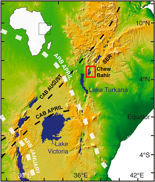
FIGURE 3. Location of the study area. The Chew Bahir basin is located in southern Ethiopia, within the southern Ethiopian rift (indicated by the red box). Rainfall in the area is determined by the annual migration of the tropical rain belt (TRB), and on inter annual time scales by the migration of the Congo air boundary (CAB). On millennial time scales rainfall shows a strong correlation with orbital precession cycles.

Rainfall in the area is determined by the migration of the tropical rain belt, which in turn follows the zenith of the Sun and results in two rainy seasons (Nicholson, 2017). During the Pleistocene, African climatic changes on millennial time scales are thought to have been caused by periodic (23–19 kyr) variations in insolation resulting from Earth’s orbital precession (e.g., Kutzbach and Street-Perrott, 1985; Berger et al., 2006). Due to the geometry of precession, changes in summer solar radiation are anti-phased between hemispheres, resulting in maximum monsoonal circulation and maximum precipitation every 19–23 kyrs in northern and southern Africa (Partridge, 1997; Trauth et al., 2003; Berger et al., 2006). In contrast, periods of increased humidity in equatorial East Africa occurred at 10–11 kyr intervals following maximum equatorial insolation in March and September (Trauth et al., 2003; Berger et al., 2006).

For this study, with its focus on calculating an age model by orbital tuning, we used the 39 band color reflectance data, which show distinct continuous cycles at ∼10–15 and ∼40 m depth intervals. Past variations in rainfall are reflected in the color of the sediments of the Chew Bahir basin, with blue-green colors during wet episodes and reddish-brown colors during dry episodes (Foerster et al., 2012). The sediment color can be primary, resulting from direct detrital sediment input, or secondary, due to diagenesis of the deposited sediments by, for example, redox processes at the sediment-water boundary under lacustrine conditions (Giosan et al., 2002 and references therein). Color reflectances within the blue green spectrum suggest reactions at the sediment-water boundary as a result of H2S production, fueled by organic matter and its consumption by sulfate reducing bacteria. H2S in the anoxic zone at the water-sediment boundary reacts with iron hydroxides, reducing any Fe³⁺ that is attached to clay minerals, bound in iron-hydroxides, or present in aqueous solution. During this process mono-sulphides and pyrite form on the lake floor and within the uppermost centimeters of sediment (Giosan et al., 2002), resulting in a spectral shift toward green/blue reflectances.

Organic matter input can derive from algal blooms within the lake and from plant material washed into the lake from the Chew Bahir catchment area. Algal blooms are in turn driven by nutrient and iron influx to the lake system (Storch and Dunham, 1986). Dissolved iron (Fe) and iron hydroxide may originate from the catchment areas at the upper eastern edge of the Chew Bahir basin, from the Teltele Plateau, and from the northeastern part of the catchment, where volcanic rocks are exposed to weathering (Foerster et al., 2012). Wind-blown dust from more distant sources may also have contributed to the nutrient and iron flux into the lake (Foerster et al., 2012). In the absence of oxygen the reduced minerals retain their diagenetic signatures and associated color reflectances until they are eventually sealed off from the lake water and possible chemical alteration by subsequent sedimentation.

We used a principal component analysis (PCA) (Pearson, 1901) to unmix the environmental factors controlling sediment color and to increase the signal-to-noise ratio, as well as to assist in interpreting the multivariate data set. The first principal component (PC1) showed similar loadings for all color bands; it was interpreted to represent the total reflectance of the sediment and was not used in this method. We Instead used PC2 (3.4% of the total variance), with positive loadings within the short wavelengths (blue reflected light), as a proxy for precipitation within the catchment area (Figures 4A,B). Complete linear unmixing was, however, not possible because the intensity values within individual wavelength bands were not perfectly Gaussian distributed.

FIGURE 4

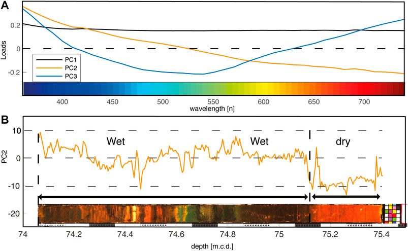
FIGURE 4. (A) To extract the environmental signal from the 39 band color reflectance data set we used a principal component analysis (PCA). The first three principal components explained 99.88% of the total variance. We used the 2nd principal component (PC2) as an environmental indicator, with positive values indicating wet periods. (B) The PC2 corresponds to red blue green color shifts that are characteristic for the sediments of the Chew Bahir core displayed at the bottom of the diagram. The colors of the core have been photographically enhanced.

We also used six Argon ages, which date the sediment at the bottom of the core to 629 ± 11 kyrs BP (one sigma error) (Roberts et al., submitted).

Results

Synthetic Data Results

We first applied the new MUBAWA technique, including the SFRA, to the synthetic data set. To visualize the frequency evolution of the synthetic data we computed a wavelet power spectrum (Figure 5A). We used the time series of orbital precession between –1.0 and 0 Ma BP from Laskar et al. (2004) as the TT and the synthetic ages as the age control points for our hypothetical core. We selected a minimum base age of 550 kyrs BP (t_min) and a maximum base age of 850 kyrs BP (t_max).

FIGURE 5

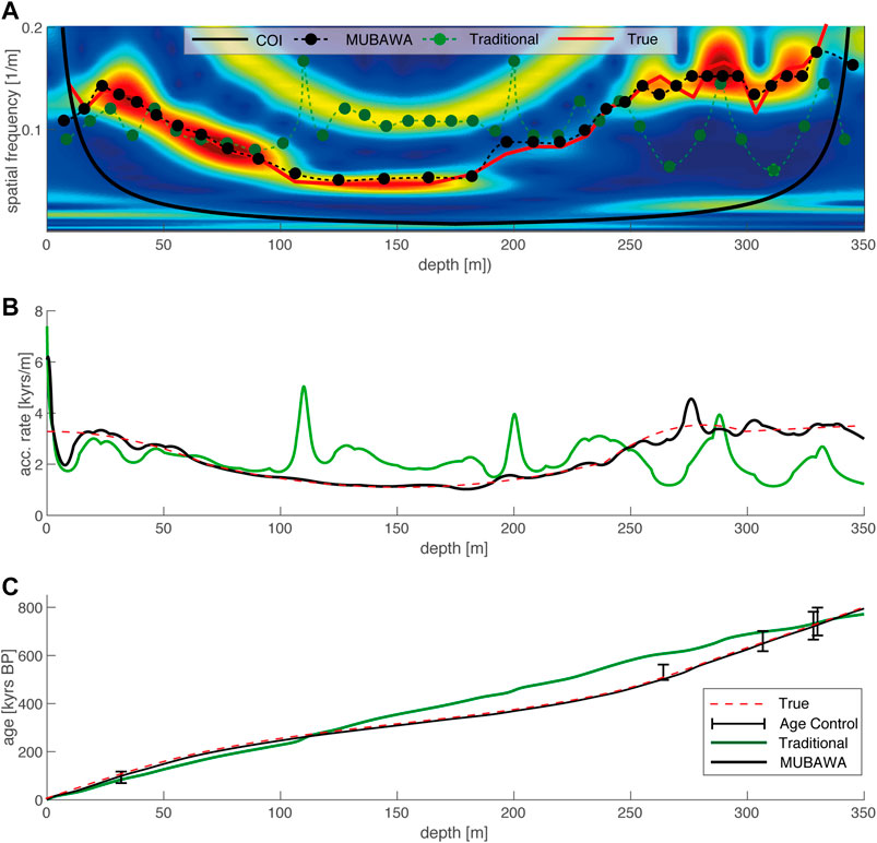
FIGURE 5. (A) The wavelet power spectrum that resulted from the CWT of the synthetic depth data demonstrates the frequency shift that has been applied by the continuous sedimentation rate changes induced by the synthetic age model. Blue colors refer to low power and red colors to high power. The green dots represent the peak distances of the filtered linear interpolated time series from the first step of the traditional tuning method. Note that where the peak distances do not follow a continuous frequency path, the traditional tuning method failed to reconstruct the synthetic sedimentation rate shown in (B). (C) The depth-age plot shows that even though the traditional method failed to reconstruct the correct sedimentation history, it yielded a similar base age.

The reconstructed accumulation rates calculated using MUBAWA age modeling largely correspond to the true (synthetic) accumulation rates (Figure 5C). A closer look at the results reveals minor deviations of the modeled accumulation rate from the true accumulation rate. The maximum age of the core determined from the synthetic data by MUBAWA age modeling, agrees well with the true maximum age.

In order to compare the results obtained from the MUBAWA method with those obtained using established tuning methods, we reconstructed the accumulation rate of the synthetic data using a traditional tuning method. We first transformed the space series into a time series with a maximum age of 800 kyrs BP. We then bandpass filtered the signal to extract the 19–23 kyr cycle that we wanted to use as the TT. Since we knew that the time series had been compressed and stretched by varying sedimentation rates, we chose a relatively wide passband with cutoff frequencies of 1/15 and 1/30 kyr⁻¹ for the filter. Finally, we aligned the maxima of the filtered time series with the minima of the TT.

Although the traditional tuning method found the correct base age for the synthetic data, it did not reconstruct the accumulation rates of the synthetic example correctly. In order to visualize which spatial frequencies resulted in the final traditionally tuned age model we used peak distances, these being the distances between each of the peaks in the filtered depth series. The variations in these distances ultimately determine the age model. A projection of the inverse of the peak distances into a wavelet power spectrum reveals which of the spatial frequencies the tuned age model is based on. The projection of the inverse of the peak distances into the wavelet power spectrum showed that the traditional method generated an age model on the basis of different spatial frequency paths from our original insolation signal. The reconstructed accumulation rates diverged from the “true“ accumulation rates where the peak distances projected into the wavelet power spectrum failed to follow the continuous spatial frequency evolution of our initial insolation signal (Figures 5A–C). The result obtained using the traditional tuning method cannot be considered satisfactory, indicating the need for a different strategy that avoids such a failure. The MUBAWA approach, which clearly follows a continuous spatial frequency path, provides such an alternative strategy.

Chew Bahir Data Results

We first created a linear age model by extrapolating through the age control at 240 m (400 kyrs). We used this age because a similar age has been obtained from the same depth in the parallel core (Roberts et al., submitted). The age model yielded a base age of 570 kyrs. We calculated a Lomb-Scargle power spectrum for the time series and computed the detection probability limit (Lomb, 1976; Scargle, 1982) (Figure 6). We found power above the detection probability limit within the precession frequency range (PFR). The possible precession cycles indicated by the simple linear age model suggested that the cycles already observed in the depth scale were indeed related to orbital precession.

FIGURE 6

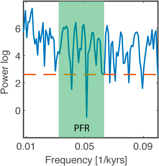
FIGURE 6. Lomb-Scargle power spectrum derived from a simple linear age model. The green color represents the precession frequency range (PFR) within which the precession frequencies can be expected to occur. The red line indicates the 95% detection probability. Frequencies within the PFR are above the detection probability suggesting that there is enough power within the precession band to run the multiband wavelet age modeling approach.

We then used the MUBAWA algorithm to calculate an orbitally tuned age model for the Chew Bahir composite core. We used PC2 from the color reflectance data, an orbital precession (according to Laskar et al., 2004) of between –1 and 0 Ma BP as the TT, and the Argon ages (together with their uncertainties) as age control points. We rejected the Argon age at a depth at 234.066 m.c.d. because of its large uncertainty and its proximity to the age date at 234.048 m.c.d., which had a smaller uncertainty. We chose 850 kyrs as the maximum base age (t_max) and 550 kyrs as the minimum base age (t_min). Preprocessing with the MUBAWA function resulted in a sampling rate of 0.3661 m⁻¹. The resulting evenly spaced subsampled data set contained 800 data points.

We then used the SFRA to approximate the frequency range that corresponded to the age control (within their uncertainty ranges) by randomly resampling the age control points to create an age model ensemble (Figure 7A). The SFRA resulted in a relatively broad frequency range in the top and bottom sections of the core, where more radiometric ages were available, and a narrower range in between (Figure 7B).

FIGURE 7

FIGURE 7. Results of the SFRA. (A) We computed 100,000 realizations (blue lines) between the randomly resampled age control points to approximate a spatial frequency range depending on the frequency of the TT and the minimum and maximum slopes of the age model ensemble. (B) The wavelet power spectrum of the adaptively filtered PC2, with blue colors indicating low power and red colors high power. The SFRA resulted in the black dashed lines that have been used to adaptively filter the depth series. The white lines are spatial frequency paths that resulted from the spatial frequency mapping. Note that we left out the age at 230 m.c.d. from the SFRA because it was very close to a better dated age with less uncertainty (close ages expand the SFRA).

We used Taner filters to adaptively bandpass filter the y-values using the upper and lower frequency limits from the SFRA, thus obtaining an adaptively filtered depth series. We performed the spatial frequency path mapping using the data from the SFRA. Ten different spatial frequency paths were mapped. All paths had different starting positions but merged after a certain depth (Figure 7B). We adaptively filtered along the frequency paths by adjusting the cutoff frequencies of the Taner filters according to the values of each individual frequency path.

Each frequency path resulted in an adaptively filtered depth series. We computed the maxima of the depth series and the minima of the TT, as negative precession resulted in an increase in monsoon strength within the study area. The interpolation points were then arranged in chronological order so that the second maximum of the filtered time series and the second minimum of the TT were assigned to each other, until the penultimate maxima of the filtered time series. We omitted the first and last maxima to avoid any edge effect of the wavelet power spectrum.

We then used a PCHIP to interpolate between the new tie-points, derived by assigning the maxima of the adaptive filtered depth series to the minima of the TT, and generated an age model for each spatial frequency path. We used the agreement between the age models resulting from the interpolation and the age control points (within their uncertainties) to evaluate the age models. We also used the Pearson correlation coefficient to rate the age models. The cutoff frequencies that eventually led to the best age model are shown in Figure 8A. The adaptively filtered time series then correlated with the TT (Figure 8B). The individual steps and their results that were applied to the depth series are shown in Figure 8C. This analysis resulted in an age model that was in agreement with most of the age control points (within their two sigma errors) and indicated a maximum age for the base of the core of 632.62 kyrs BP (Figure 9). We applied our MUBAWA-based age model to the PC2 of the 39 band color reflectance record (Figure 10A).; the wavelet power spectrum of the resulting time series showed significant orbital cycles with periods of 100, 60, 19–25, 10–15, and 5 kyrs (Figure 10B).

FIGURE 8

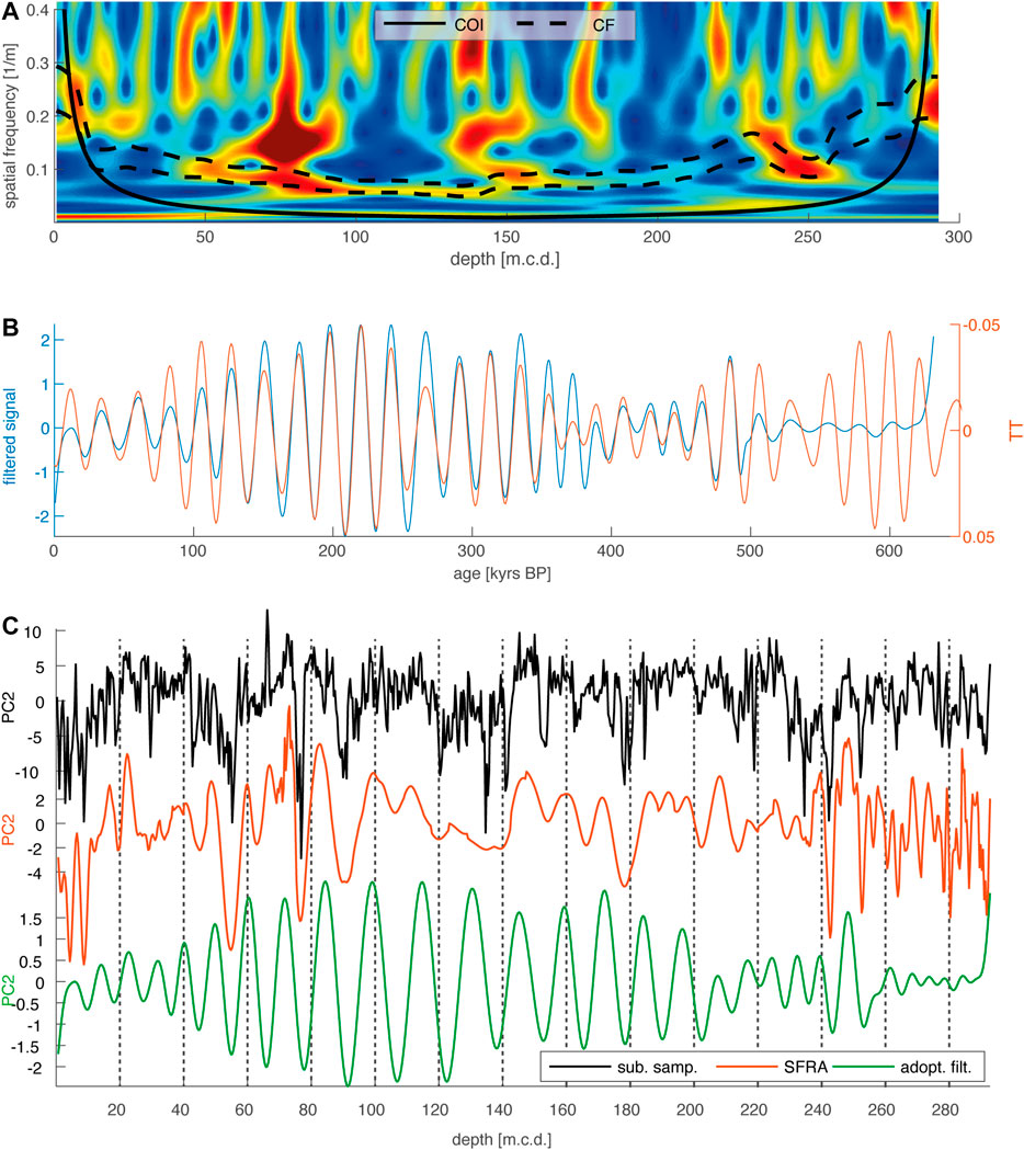
FIGURE 8. (A) Each frequency path was converted into an upper and lower cutoff frequency to adaptively filter along the spatial frequency path. The cutoff frequencies that resulted in the best age model are shown as black dashed lines. (B) The peaks of the adoptively filtered signal were consecutively projected onto the peaks of the tuning target (TT) to generate an age model. (C) The results of each processing step are shown from top to bottom, starting with the sub sampled PC2, the results of the SFRA, and the adoptively filtered depth series.

FIGURE 9

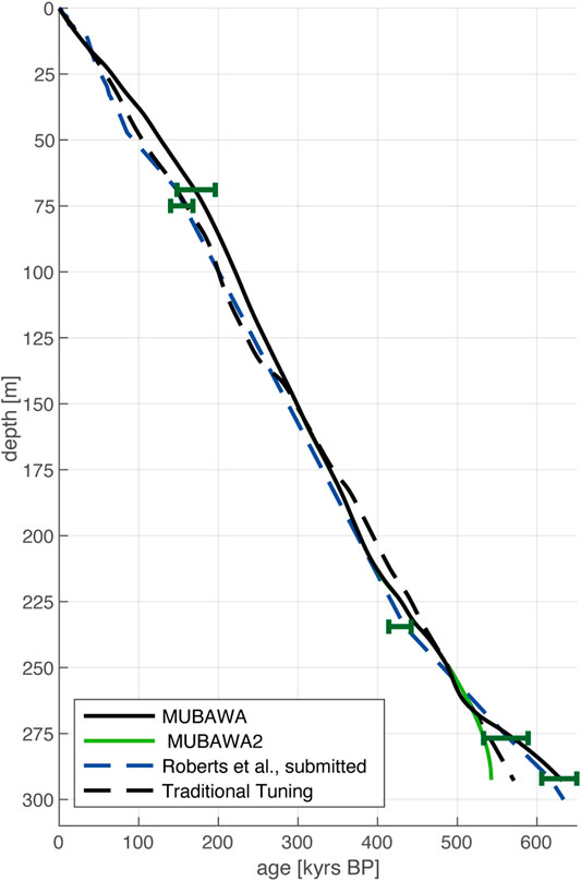
FIGURE 9. Two additional age models have been developed for the Chew Bahir project: a direct-dated age model (Roberts et al., submitted.) and a traditionally tuned age model. Note that the multiband wavelet age modeling (MUBAWA) age model is in strong agreement with the age controls. MUBAWA2 represents an additional age model that has resulted from one of the frequency paths, but was ranked second.

FIGURE 10

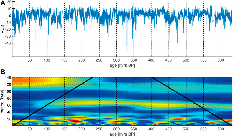
FIGURE 10. (A) Resulting time series. The multiband wavelet age modeling age model was used to convert PC2 depth series into a time series, as shown. (B) Wavelet power spectrum, with the age along the x-axis and the period along the y-axis. The colors indicate the power of the cycle, with red colors for high power and blue colors for low power. The wavelet power spectrum computed from the PC2 time series shows the anticipated precession cycles, since the age model was tuned to that cycle. The continuity of the longer wavelength periods at 60 and 100 kyrs shows that the tuning has been successful.

In order to further compare our MUBAWA approach with the traditional method we also applied the previously described traditional tuning method to the Chew Bahir data. For this we first assumed a preliminary base age of 500 kyrs. We generated a time series based on this simple linear preliminary model and then applied a relatively wide bandpass filter with cutoff frequencies of 1/28 and 1/16 kyr⁻¹. Both methods can be seen from the peak distances to operate in the same frequency domain (Figure 11A). The accumulation rates show a strong correlation with the peak distances (Figure 11B). The age-depth gradients differ only slightly and remain within the uncertainties of the Argon ages (Figure 11C).

FIGURE 11

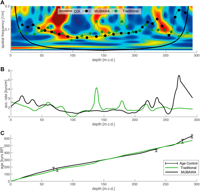
FIGURE 11. (A) Wavelet power spectrum, with frequency along the y-axis and depth along the x-axis. The power is indicated by color, with red colors for high power and blue colors for low power. The peak distances can be used to compare the traditional approach with the new multiband wavelet age modeling (MUBAWA) approach. Both methods follow approximately the same cycle until 230 m.c.d., after which they show marked differences. (B) Where the peak distances differ in (A), the accumulation rates are significantly different. (C) The two age models only vary insignificantly in the depth age plot. However, the MUBAWA model tracks to higher frequencies below 250 m.c.d. on, which allows it to reach the argon age at the base of the composite core.

Discussion

We have developed a new age modeling technique that is specifically suited to climate records with distinct orbital cycles and limited age control. The approach involves statistical analysis of an age model ensemble to delimit the spatial frequency range of the targeted orbital frequency. It uses a wavelet power spectrum derived from the CWT to trace the evolution of the orbital frequency and ultimately adapt the bandpass filter to its variations, allowing for continuous long-term changes in sedimentation rates. This new technique is in improvement on traditional tuning techniques that use a single bandpass filter to tune paleoclimate records. The method depends on a number of parameters that may need to be adjusted when using data sets other than those presented herein. These include the amount of weighting, the sampling rate, and the bandwidth of the adaptive filter.

By applying a traditional tuning method to synthetic data we have shown that when the data to be tuned are characterized by continuous long-term changes in sedimentation rates, jumps occur in the spatial frequency that lead to misinterpretation of the spectral data and ultimately to a false age model. We have shown that such misinterpretation of the data set can be detected by plotting the peak distances of the filtered, but untuned, time series into a wavelet power spectrum of the untuned raw spatial data. If the peak distances correspond to a continuous frequency evolution, the traditional tuning method will produce accurate results. If, however, the peak distances show no match with a continuous frequency evolution the method will fail to deliver accurate results. It is specifically for cases resembling the synthetic data, which are common in nature, that we have developed the MUBAWA method. The MUBAWA technique has demonstrated its ability to handle such special circumstances by correctly solving the synthetic example.

Application of the MUBAWA approach to the Chew Bahir record and using PC2 from its color reflectance data set has produced a tuned age model that is in strong agreement with independent age controls and shows continuous orbital cycles in the wavelet power spectrum. As expected, the tuning revealed particularly distinct cycles corresponding to frequencies contained in the TT. Furthermore, a set of higher frequencies with periods of ∼5 kyr that, according to Berger et al. (2006), are attributable to fundamental harmonics, can be identified in the tuned time series. The occurrence of a distinct ∼10–15 kyr cycle suggests half precessional forcing of the Chew Bahir environmental conditions, as previously suggested by Berger et al. (2006), Berger et al. (1997), and Trauth et al. (2003). We also identified a distinct continuous 63 kyr cycle. Its occurrence can possibly be attributed to heterodynes, as described by Clemens et al. (2010), Clemens et al. (2018) and recently identified in South Asian precipitation records (Gebregiorgis et al., 2018). We also recognized a continuous 100 kyr cycle that can be ascribed to eccentricity in the earth’s orbit (Figure 10).

We also created a traditional tuned age model (according to common practice) using the Chew Bahir data, for comparison with the MUBAWA age model. The result again revealed a strong agreement with the age control points (Figure 11C), with the exception of the oldest age at the base of the composite core. This model would certainly be a satisfactory result for users of established tuning methods. To compare the resulting filtered depth series of the MUBAWA approach with the traditionally tuned filtered depth series we plotted the peak distances of the traditionally tuned filtered depth series and the peak distances of the MUBAWA filtered depth series into the wavelet power spectrum (Figure 11A), as demonstrated previously for the synthetic example.

The peak distance analysis revealed that, despite the agreement with the age control points and the increase in the power of the eccentricity cycle, a discontinuous spatial frequency evolution had been used through parts of the composite core. The synthetic data example showed that such jumps in spatial frequency can lead to misinterpretations (Figure 11A). Although real data are far more complex and the exact sedimentation history of such data is largely unknown, we believe that the continuity assumption in our MUBAWA approach enables it to make an important contribution to tuning-based age modeling.

Conclusion

We have demonstrated in our synthetic example that tuning methods using stationary bandpass filters have difficulty reconstructing the correct accumulation history, whereas the MUBAWA algorithm presented herein, using the CWT to track a continuous frequency evolution, yielded the correct solution. Application of the MUBAWA approach to the Chew Bahir record and the PC2 of its color reflectance data revealed that the method is also applicable to real climate data sets. A comparison with traditional tuning showed that, whereas the traditional tuning method is limited to rather linear age models, the MUBAWA approach is capable of detecting and taking into account continuous long-term changes in sedimentation rates. Not only was the MUBAWA-generated age model in good agreement with the available age control points (within their uncertainties), but it was also able to reconstruct continuous orbital cycles, as shown in the wavelet power spectrum. We recommend the MUBAWA approach for use with a wide range of climate data sets that require sophisticated tuning methods.

Data Availability Statement

The original contributions presented in the study are included in the article/Supplementary Material, further inquiries can be directed to the corresponding author.

Author Contributions

WD is the lead author of the publication and was involved in all crucial steps from initiation of the first ideas, implementation of the statistical analysis, and the writing process. KH and NB were mainly involved in supporting the development of the methods section. MT, as well as NM have accompanied the entire process and supported the development of the work on numerous issues ranging from code implementation to the interpretation of climate processes. AD provided the radiometric ages.

Funding

Support for HSPDP has been provided by the National Science Foundation (NSF) grants and the International Continental Drilling Program (ICDP). Support for CBDP has been provided by Germany Research Foundation (DFG) through the Priority Program SPP 1006 ICDP (SCHA 472/13 and /18, TR 419/8, /10 and /16) and the CRC 806 Research Project “Our way to Europe” Project Number 57444011. Support has also been received from the UK Natural Environment Research Council (NERC, NE/K014560/1, IP/1623/0516). We also thank the Ethiopian permitting authorities to issue permits for drilling in the Chew Bahir basin. We also thank the Hammar people for the local assistance during drilling operations. We thank DOSECC Exploration Services for drilling supervision and Ethio Der pvt. Ltd. Co. for providing logistical support during drilling. Initial core processing and sampling were conducted at the US National Lacustrine Core Facility (LacCore) at the University of Minnesota. S.K.B. has received further financial support from the University of Potsdam Open Topic Postdoc Program.

Conflict of Interest

The authors declare that the research was conducted in the absence of any commercial or financial relationships that could be construed as a potential conflict of interest.

Acknowledgments

We thank Christopher Bronk Ramsey, Melissa Chapot, Christine S. Lane, Helen M. Roberts and Céline Vidal for discussions on the geochronology and age modeling. This is publication ## of the Hominin Sites and Paleolakes Drilling Project.

Supplementary Material

The Supplementary Material for this article can be found online at: https://www.frontiersin.org/articles/10.3389/feart.2021.594047/full#supplementary-material.

References

Addison, P. S. (2017). The illustrated wavelet transform handbook: introductory theory and applications in science, engineering, medicine and finance. 2nd Ed. India: CRC Press.

Berger, A., Loutre, M. F., and Mclntyre, A. (1997). Intertropical latitudes and precessional and half-precessional cycles. Science 278 (5342), 1476–1478. doi:10.1126/science.278.5342.1476

CrossRef Full Text | Google Scholar

Berger, A., Loutre, M. F., and Mélice, J. L. (2006). Equatorial insolation: from precession harmonics to eccentricity frequencies. Clim. Past 2 (2), 131–136. doi:10.5194/cp-2-131-2006

CrossRef Full Text | Google Scholar

Campisano, F. A., Drake, A. J., Floyd, M. S., Hui, D. T., Owczarczyk, P., Tiner, M. D., et al. (2017). U.S. Patent Application No. 14/879,269.

Cheung, W. H., Senay, G. B., and Singh, A. (2008). Trends and spatial distribution of annual and seasonal rainfall in Ethiopia. Int. J. Climatol. 28 (13), 1723–1734. doi:10.1002/joc.1623

CrossRef Full Text | Google Scholar

Clemens, S. C., Holbourn, A., Kubota, Y., Lee, K. E., Liu, Z., Chen, G., et al. (2018). Precession-band variance missing from East Asian monsoon runoff. Nat. Commun. 9 (1), 3364. doi:10.1038/s41467-018-05814-0

PubMed Abstract | CrossRef Full Text | Google Scholar

Clemens, S. C., Prell, W. L., and Sun, Y. (2010). Orbital - scale timing and mechanisms driving Late Pleistocene Indo - Asian summer monsoons: reinterpreting cave speleothemδ18O. Paleoceanography 25 (4). doi:10.1029/2010pa001926

CrossRef Full Text | Google Scholar

Cohen, A., Campisano, C., Arrowsmith, R., Asrat, A., Behrensmeyer, A. K., Deino, A., et al. (2016). The Hominin Sites and Paleolakes Drilling Project: inferring the environmental context of human evolution from eastern African rift lake deposits. Sci. Drill. 21, 1–16. doi:10.5194/sd-21-1-2016

CrossRef Full Text | Google Scholar

Davidson, A. (1983). The Omo River project: reconnaissance geology and geochemistry of parts of Ilubabor, Kefa, Gemu Gofa and Sidamo. Ethiopian Institute of Geological Surveys Bulletin 2, 1e89.

Google Scholar

Ebinger, C. J., Yemane, T., Harding, D. J., Tesfaye, S., Kelley, S., and Rex, D. C. (2000). Rift deflection, migration, and propagation: linkage of the Ethiopian and Eastern rifts, Africa. Geol. Soc. Am. Bull. 112 (2), 163–176. doi:10.1130/0016-7606(2000)112<163:rdmapl>2.0.co;2

CrossRef Full Text | Google Scholar

Foerster, , et al. submitted.

Foerster, V., Junginger, A., Langkamp, O., Gebru, T., Asrat, A., Umer, M., et al. (2012). Climatic change recorded in the sediments of the Chew Bahir basin, southern Ethiopia, during the last 45,000 years. Quat. Int. 274, 25–37. doi:10.1016/j.quaint.2012.06.028

CrossRef Full Text | Google Scholar

Fritsch, F. N., and Carlson, R. E. (1980). Monotone piecewise cubic interpolation. SIAM J. Numer. Anal. 17 (2), 238–246. doi:10.1137/0717021

CrossRef Full Text | Google Scholar

Gebregiorgis, D., Hathorne, E. C., Giosan, L., Clemens, S., Nürnberg, D., and Frank, M. (2018). Southern Hemisphere forcing of South Asian monsoon precipitation over the past ∼1 million years. Nat. Commun. 9 (1), 4702. doi:10.1038/s41467-018-07076-2

PubMed Abstract | CrossRef Full Text | Google Scholar

Giosan, L., Flood, R. D., and Aller, R. C. (2002). Paleoceanographic significance of sediment color on western North Atlantic drifts: I. Origin of color. Mar. Geol. 189 (1-2), 25–41. doi:10.1016/s0025-3227(02)00321-3

CrossRef Full Text | Google Scholar

Grant, K. M., Rohling, E. J., Westerhold, T., Zabel, M., Heslop, D., Konijnendijk, T., et al. (2017). A 3 million year index for North African humidity/aridity and the implication of potential pan-African Humid periods. Quat. Sci. Rev. 171, 100–118. doi:10.1016/j.quascirev.2017.07.005

CrossRef Full Text | Google Scholar

Hays, J. D., Imbrie, J., and Shackleton, N. J. (1976a). Variations in the earth's orbit: pacemaker of the ice ages. Science 194, 1121–1132. doi:10.1126/science.194.4270.1121

PubMed Abstract | CrossRef Full Text | Google Scholar

Hays, J. D., Imbrie, J., and Shackleton, N. J. (1976b). Variations in the Earth's orbit: pacemaker of the ice ages. Washington, DC: American Association for the Advancement of Science.

Hinnov, L. A. (2013). Cyclostratigraphy and its revolutionizing applications in the earth and planetary sciences. Geol. Sci. Am. Bull. 125 (11–12), 1703–1734. doi:10.1130/b30934.1

CrossRef Full Text | Google Scholar

Hotelling, H. (1933). Analysis of a complex of statistical variables into principal components. J. Educ. Psychol. 24 (6), 417–441. doi:10.1037/h0071325

CrossRef Full Text | Google Scholar

Imbrie, J., and Imbrie, J. Z. (1980). Modeling the climatic response to orbital variations. Science 207 (4434), 943–953. doi:10.1126/science.207.4434.943

PubMed Abstract | CrossRef Full Text | Google Scholar

Kutzbach, J. E., and Street-Perrott, F. A. (1985). Milankovitch forcing of fluctuations in the level of tropical lakes from 18 to 0 kyr BP. Nature 317 (6033), 130–134. doi:10.1038/317130a0

CrossRef Full Text | Google Scholar

Laskar, J., Robutel, P., Joutel, F., Gastineau, M., Correia, A. C. M., and Levrard, B. (2004). A long-term numerical solution for the insolation quantities of the Earth. Astron. Astrophys. 428, 261–285. Available at: http://vo.imcce.fr/insola/earth/online/earth/online/. doi:10.1051/0004-6361:20041335

CrossRef Full Text | Google Scholar

Lau, K.-M., and Weng, H. (1995). Climate signal detection using wavelet transform: how to make a time series sing. Bull. Am. Meteorol. Soc. 76 (12), 2391–2402. doi:10.1175/1520-0477(1995)076<2391:csduwt>2.0.co;2

CrossRef Full Text | Google Scholar

Lomb, N. R. (1976). Least-squares frequency analysis of unequally spaced data. Astrophys. Space Sci. 39 (2), 447–462. doi:10.1007/bf00648343

CrossRef Full Text | Google Scholar

Martinson, D. G., Pisias, N. G., Hays, J. D., Imbrie, J., Moore, T. C., and Shackleton, N. J. (1987). Age dating and the orbital theory of the ice ages: development of a high-resolution 0 to 300,000-year chronostratigraphy. Quat. res. 27 (1), 1–29. doi:10.1016/0033-5894(87)90046-9

CrossRef Full Text | Google Scholar

MathWorks (2020a). MATLAB signal processing toolbox – User’s guide. Natick, MA: The MathWorks, Inc.

Meyers, S. R., Sageman, B. B., and Hinnov, L. A. (2001). Integrated quantitative stratigraphy of the Cenomanian-Turonian Bridge Creek Limestone Member using evolutive harmonic analysis and stratigraphic modeling. J. Sediment. Res. 71 (4), 628–644. doi:10.1306/012401710628

CrossRef Full Text | Google Scholar

Meyers, S. R., and Sageman, B. B. (2007). Quantification of deep-time orbital forcing by average spectral misfit. Am. J. Sci. 307 (5), 773–792. doi:10.2475/05.2007.01

CrossRef Full Text | Google Scholar

Meyers, S. R. (2015). The evaluation of eccentricity-related amplitude modulation and bundling in paleoclimate data: an inverse approach for astrochronologic testing and time scale optimization. Paleoceanography 30 (12), 1625–1640. doi:10.1002/2015pa002850

CrossRef Full Text | Google Scholar

Muller, R. A., and MacDonald, G. J. (2002). Ice ages and astronomical causes: data, spectral analysis and mechanisms. London, UK: Springer Science & Business Media.

Nicholson, S. E. (2017). Climate and climatic variability of rainfall over eastern Africa. Rev. Geophys. 55 (3), 590–635. doi:10.1002/2016rg000544

CrossRef Full Text | Google Scholar

Park, J., and Herbert, T. D. (1987). Hunting for paleoclimatic periodicities in a geologic time series with an uncertain time scale. J. Geophys. Res. 92 (B13), 14027–14040. doi:10.1029/jb092ib13p14027

CrossRef Full Text | Google Scholar

Partridge, T. C. (1997). Cainozoic environmental change in southern Africa, with special emphasis on the last 200 000 years. Prog. Phys. Geogr. Earth Environ. 21 (1), 3–22. doi:10.1177/030913339702100102

CrossRef Full Text | Google Scholar

Pearson, K. (1901). LIII. On lines and planes of closest fit to systems of points in space. The London, Edinburgh, and Dublin Philos. Mag. J. Sci. 2 (11), 559–572. doi:10.1080/14786440109462720

CrossRef Full Text | Google Scholar

Pik, R., Marty, B., Carignan, J., Yirgu, G., and Ayalew, T. (2008). Timing of East African Rift development in southern Ethiopia: implication for mantle plume activity and evolution of topography. Geology 36 (2), 167–170. doi:10.1130/g24233a.1

CrossRef Full Text | Google Scholar

Pisias, N. G., Martinson, D. G., Moore, T. C., Shackleton, N. J., Prell, W., Hays, J., et al. (1984). High resolution stratigraphic correlation of benthic oxygen isotopic records spanning the last 300,000 years. Mar. Geol. 56 (1–4), 119–136. doi:10.1016/0025-3227(84)90009-4

CrossRef Full Text | Google Scholar

Raymo, M. E., Oppo, D. W., and Curry, W. (1997). The Mid-Pleistocene climate transition: a deep sea carbon isotopic perspective. Paleoceanography 12 (4), 546–559. doi:10.1029/97pa01019

CrossRef Full Text | Google Scholar

Roberts, , et al. (2020). Interactive comment on “New analytical and data evaluation protocols to improve the reliability of U-Pb LA-ICP-MS carbonate dating” by Marcel Guillong et al. Geochronol. Dis. C1–C7. doi:10.5194/gchron-2019-20-sc1

CrossRef Full Text | Google Scholar

Saji, N. H., Goswami, B. N., Vinayachandran, P. N., and Yamagata, T. (1999). A dipole mode in the tropical Indian Ocean. Nature 401 (6751), 360–363. doi:10.1038/43854

PubMed Abstract | CrossRef Full Text | Google Scholar

Scargle, J. D. (1982). Studies in astronomical time series analysis. II - statistical aspects of spectral analysis of unevenly spaced data. Astrophys. J. 263, 835–853. doi:10.1086/160554

CrossRef Full Text | Google Scholar

Segele, Z. T., Richman, M. B., Leslie, L. M., and Lamb, P. J. (2015). Seasonal-to-interannual variability of Ethiopia/horn of Africa monsoon. Part II: statistical multimodel ensemble rainfall predictions. J. Clim. 28 (9), 3511–3536. doi:10.1175/jcli-d-14-00476.1

CrossRef Full Text | Google Scholar

Seleshi, Y., and Zanke, U. (2004). Recent changes in rainfall and rainy days in Ethiopia. Int. J. Climatol. 24 (8), 973–983. doi:10.1002/joc.1052

CrossRef Full Text | Google Scholar

Sinnesael, M., Zivanovic, M., De Vleeschouwer, D., and Claeys, P. (2018). Spectral moments in cyclostratigraphy: advantages and disadvantages compared to more classic approaches. Paleoceano. Paleoclimatol. 33 (5), 493–510. doi:10.1029/2017pa003293

CrossRef Full Text | Google Scholar

Storch, T. A., and Dunham, V. L., (1986). Iron-mediated changes in the growth of lake erie phytoplankton and axenic algal cultures. J. Phycol. 22 (2), 109–117. doi:10.1111/j.1529-8817.1986.tb04152.x

CrossRef Full Text | Google Scholar

Taner, M. T. (1992). Attributes revisted. Technical Report. Rock solid images, Inc. Available at: http://www.rocksolidimages.com/attributes-revisited/#_Toc328470897.

Tiedemann, R., Sarnthein, M., and Shackleton, N. J. (1994). Astronomic timescale for the pliocene atlantic δ18O and dust flux records of ocean drilling program site 659. Paleoceanography 9 (4), 619–638. doi:10.1029/94pa00208

CrossRef Full Text | Google Scholar

Torrence, C., and Compo, G. P. (1998). A practical guide to wavelet analysis. Bull. Am. Meteorol. Soc. 79 (1), 61–78. doi:10.1175/1520-0477(1998)079<0061:apgtwa>2.0.co;2

CrossRef Full Text | Google Scholar

Trauth, M. H., Deino, A. L., Bergner, A. G., and Strecker, M. R. (2003). East African climate change and orbital forcing during the last 175 kyr BP. Earth Planet Sci. Lett. 206 (3–4), 297–313. doi:10.1016/s0012-821x(02)01105-6

CrossRef Full Text | Google Scholar

Wagner, B., Vogel, H., Francke, A., Friedrich, T., Donders, T., Lacey, J. H., et al. 2019). Mediterranean winter rainfall in phase with African monsoons during the past 1.36 million years. Nature 573, 256–260. doi:10.1038/s41586-019-1529-0

PubMed Abstract | CrossRef Full Text | Google Scholar

Woldegabriel, G., Aronson, J. L., and Walter, R. C. (1990). Geology, geochronology, and rift basin development in the central sector of the Main Ethiopia Rift. Geol. Soc. Am. Bull. 102 (4), 439–458. doi:10.1130/0016-7606(1990)102<0439:ggarbd>2.3.co;2

CrossRef Full Text | Google Scholar

Zeeden, C., Kaboth, S., Hilgen, F. J., and Laskar, J. (2018). Taner filter settings and automatic correlation optimisation for cyclostratigraphic studies. Comput. Geosci. 119, 18–28. doi:10.1016/j.cageo.2018.06.005

CrossRef Full Text | Google Scholar