Disentangle Kinetic From Equilibrium Fractionation Using Primary (δ17O, δ18O, δD) and Secondary (Δ17O, dex) Stable Isotope Parameters on Samples From the Swiss Precipitation Network

Introduction

Water isotope ratio measurements are among the first determinations done. The history reaches back to the early days of mass spectrometry (Aston, 1942; Ney and Mann, 1946; Nier and Roberts, 1951; Dibeler, 1954). Applications of mass spectrometry evolved rapidly with several developments on preparation systems of diverse samples (Epstein et al., 1951; den Boer and Borg, 1952; Dostrovsky and Klein, 1952; Friedman and Irsa, 1952; Graff and Rittenberg, 1952; Chinard and Enns, 1953; Dubbs, 1953; Washburn et al., 1953). One important application was the reconstruction of climate conditions based on carbonate oxygen isotopes (Urey et al., 1951). Over the many decades it remained an important research topic due to its relevance in many different fields such as hydrology (Aggarwal et al., 2005), meteorology (Yoshimura, 2015), geology (Andrews, 2006), cryosphere (Moser and Stichler, 1980; Masson-Delmotte et al., 2008), biology (Griffiths, 1998; Diefendorf and Freimuth, 2017), chemistry and geochemistry (Bird and Ascough, 2012; Klaus and McDonnell, 2013) and lately of course for applications in the field of climate (Galewsky et al., 2016) and environmental change of the Earth (Cernusak et al., 2016; Allen et al., 2017). Nowadays isotope ratio measurements are standard parameters to be determined in order to characterize the system under investigation, but so-called secondary parameter came into play such as the deuterium excess, d_ex defined as d_ex = δD–8·δ¹⁸O (Stenni et al., 2010; Aemisegger et al., 2014; Pfahl and Sodemann, 2014; Tanoue and Ichiyanagi, 2016), as well as the Δ¹⁷O, for its definition see Eq. 4 below, (Schoenemann et al., 2013; Steig et al., 2014; Barkan et al., 2015; Uechi and Uemura, 2019). Both parameters are scaled differences of primary isotope ratios. Δ¹⁷O, being only dependent on oxygen isotope ratios, is less dependent on temperature compared to d_ex, which itself is a combination of hydrogen and oxygen isotope ratios. This fact originates from a close cancellation of the temperature dependence among different isotope ratios of the same element compared to a different isotope ratios of different elements, i.e. d_ex. This independence of temperature allows us now to investigate dependencies on other parameters such as the relative humidity linked to kinetic fractionation effects that occur during water vapor diffusion through unsaturated air. Hence, Δ¹⁷O measurements has the potential to differentiate between kinetic and equilibrium fractionation influence. This opens up a wide range of applications 1) on the hydrological cycle, e.g. humidity conditions at water vapor source locations, influence of re-evaporation on land from lakes and rivers; 2) in biological systems regarding transpiration processes; 3) in paleoclimatology to reconstruct temperature and humidity conditions at the site of precipitation and source of the formed water vapor; 4) in stratosphere-troposphere exchanges and many more.

In this study, we will elaborate on this partitioning of the two fractionations on measurements done on samples from the Swiss network of isotope ratios on precipitation, ISOT (Schotterer et al., 2010). Materials and Methods briefly describes the sites, their characteristics, and the methods of how the isotope ratio measurements are done. Furthermore, it recalls already established equations focusing on Δ¹⁷O and discusses dependencies of the exponent that relates the two oxygen isotope ratios δ¹⁷O and δ¹⁸O, namely on ¹⁸R_s, the proportionality constants A between ¹⁷R and ¹⁸R for sample and standard materials (A_s, A_r) and Δ¹⁷O. In the results section, we discuss three theoretical experiments that we compare with corresponding data. These include 1) a two component mixing, 2) mixing of kinetic and equilibrium fractionation and 3) application of the Rayleigh model to data from the ISOT network. The results of these comparisons are discussed in Discussion.

Materials and Methods

Sample and Site Selection and Characteristics of Sites Used in This Study

Monthly integrated samples from the ISOT-network form the base for the comparison with the Rayleigh model application. Measurements have been performed so far for the two time period January 1990 to December 1993 and January 2002 to December 2004 for all stations except Jungfraujoch (JFJ) for which the complete series between January 1983 to December 2011 were measured. We selected seven stations, i.e. Basel, Bern, Meiringen, Guttannen, Grimsel, JFJ, and Locarno on a North to South transect of Switzerland that corresponds simultaneously to an altitude transect from 292 (Basel) to 3,580 (JFJ) meters above sea level. Therefore, we can investigate influences on water isotopes over a mean annual temperature from −7.9°C to +12.4°C. Since the Alps form a natural barrier for wind systems, we also can compare Atlantic to Mediterranean water vapor sources.

Measurements Methods

Measurements that are used in this study have been obtained using a Picarro Cavity Ring Down spectrometer (L-2140-i) (Steig et al., 2014). The measurements have been conducted in 2013 and 2014. Samples were injected at least 6 times from which at least the first two were discarded. Before and after 10 samples standard waters for calibrations are measured, namely Eiswasser and B_SLAP that are tightly linked to an international scale (Schoenemann et al., 2013; Affolter et al., 2015). Internal precisions (standard deviation of replicates from one sample container) are <0.05, <0.04, <0.5 and <18 permeg for δ¹⁸O, δ¹⁷O, δD and Δ¹⁷O, whereas external precisions (standard deviations of replicated sample means of different sample containers) and trueness (deviations of means to assigned values) are <0.1, <0.06, <0.4 and <9 permeg and <0.3, <0.01, <1.1 and <11 permeg for δ¹⁸O, δ¹⁷O, δD and Δ¹⁷O. Furthermore, in this study, we used internal water standards for mixing experiments that have been characterized to the international water scale VSMOW and SLAP. These internal standards include Meerwasser, Bern_DomeC, and B_SLAP. Meerwasser has a δ¹⁸O value of close to zero permil on the VSMOW scale, whereas the other two are close to SLAP. Furthermore, B_SLAP carries a very different Δ¹⁷O compared to the other two standards that allow us to investigate the equations introduced under General equations used for isotope ratio measurements with a special focus on Δ¹⁷O below.

General Equations Used for Isotope Ratio Measurements with a Special Focus on Δ¹⁷O

Oxygen isotope ratios are closely linked to each other in the form of

${{\displaystyle {}^{17}R}}_i=A_i\cdot {{\displaystyle {}^{18}R}}_i^{{\lambda }_i},(1)$

where ¹⁷R_i corresponds to the ratio of [¹⁷O]_i/[¹⁶O]_i and ¹⁸R_i to [¹⁸O]_i/[¹⁶O]_i, the exponent λ_i describes the relationship whereas A_i corresponds to a proportionality constants with i for s (sample) or r (reference, standard or an arbitrarily chosen operational parameter by the science community).

As discussed in Kaiser (Kaiser, 2008), there are five different types of relationships possible for the isotope composition of a sample and a reference. We do not repeat these evaluations but just recall some of the cases, here. For a detailed understanding, the reader is advised to read the publication of Kaiser. The first case corresponds to the generally assumed case of a sample that follows exactly the same relationship as the standard, i.e. the proportionality constant A_s = A_r = A and the exponent λ_s = λ_r = λ are the same. Therefore, it follows by division of Eq. 1 for the sample and the reference that

$\frac{{{\displaystyle {}^{17}R}}_s}{{{\displaystyle {}^{17}R}}_r}=1+{\delta }^{17}={\left(1+{\delta }^{18}\right)}^{\lambda }={\left(\frac{{{\displaystyle {}^{18}R}}_s}{{{\displaystyle {}^{18}R}}_r}\right)}^{\lambda }.(2)$

As discussed by Angert et al., (Angert et al., 2004), it should be noted that a mass dependent relationship between a substrate and a product is characterized by $\theta =\ln \left({}^{17}\alpha \right)/\ln \left({}^{18}\alpha \right)$ with

$\begin{array}{l}{}^{17}\alpha =\frac{{{\displaystyle {}^{17}R}}_{\text{product}}}{{{\displaystyle {}^{17}R}}_{\text{substrate}}},\\ {}^{18}\alpha =\frac{{{\displaystyle {}^{18}R}}_{\text{product}}}{{{\displaystyle {}^{18}R}}_{\text{substrate}}},\end{array}$

when the sample and reference corresponds to the product and substrate, respectively, then in this case Eq. 2 reads

${}^{17}\alpha =\frac{{{\displaystyle {}^{17}R}}_{\text{product}}}{{{\displaystyle {}^{17}R}}_{\text{substrate}}}=1+{\delta }^{17}={\left(1+{\delta }^{18}\right)}^{\theta }={\left(\frac{{{\displaystyle {}^{18}R}}_{\text{product}}}{{{\displaystyle {}^{18}R}}_{\text{substrate}}}\right)}^{\theta }={{\displaystyle {}^{18}\alpha }}^{\lambda }.$

And hence $\theta =\lambda$.

Rewriting Eq. 2 in logarithmic form reads

$\ln \left({\delta }^{17}+1\right)=\lambda \cdot \ln \left({\delta }^{18}+1\right).(3)$

Since it has been shown that natural processes follow different power laws, i. e different exponents, one had to define an exponent to express deviations from it. The chosen value was 0.528 for $\lambda$, corresponding to the value obtained for precipitation samples (Meijer and Li, 1998; Assonov and Brenninkmeijer, 2003). The ¹⁷O_excess value, here written as Δ¹⁷O, is therefore defined as:

${\Delta }^{17}O=\ln \left({\delta }^{17}+1\right)-0.528\cdot \ln \left({\delta }^{18}+1\right).(4)$

A more logical definition would have been to use Eq. 5, though the deviations are only important for very high values of Δ$\text{'}$¹⁷O as shown by the Taylor expansion of Eq. 5, i.e. Eq. 6.

$\ln \left(1+{{\Delta }^{\prime }}^{17}O\right)=\ln \left({\delta }^{17}+1\right)-0.528\cdot \ln \left({\delta }^{18}+1\right),(5)$

$\ln \left(1+{{\Delta }^{\prime }}^{17}O\right)={{\Delta }^{\prime }}^{17}O-\frac{{\left({{\Delta }^{\prime }}^{17}O\right)}^2}{2}+\frac{{\left({{\Delta }^{\prime }}^{17}O\right)}^3}{3}.(6)$

As can be seen by comparing Eqs. 4, 5 there is a slight difference between them in the order of the squared Δ$\text{'}$¹⁷O, which is generally neglectable and may only become relevant for samples that deviate significantly from the relationship with the exponent 0.528, i.e. stratospheric samples for which λ is close to unity. We can reformulate Eq. 5 such that it has the same mathematical form as the normal delta notation for isotope ratios, yet based on ratios of isotope ratios.

${{\Delta }^{\prime }}^{17}O=\frac{{\delta }^{17}+1}{{\left({\delta }^{18}+1\right)}^{0.528}}-1=\frac{{{\displaystyle {}^{17}R}}_s/{{\displaystyle {}^{17}R}}_r}{{\left({{\displaystyle {}^{18}R}}_s/{{\displaystyle {}^{18}R}}_r\right)}^{0.528}}-1=\left(\frac{R{\text{'}}_s}{R{\text{'}}_r}-1\right),(7)$

with $R{\text{'}}_s={{\displaystyle {}^{17}R}}_s/{\left({{\displaystyle {}^{18}R}}_s\right)}^{0.528}$ and $R{\text{'}}_r={{\displaystyle {}^{17}R}}_r/{\left({{\displaystyle {}^{18}R}}_r\right)}^{0.528}$

Δ$\text{'}$¹⁷O becomes zero when the exponent λ_s in Eq. 1 is 0.528. If this is not the case Eq. 7 can be rewritten as

${{\Delta }^{\prime }}^{17}O=\frac{{\delta }^{17}+1}{{\left({\delta }^{18}+1\right)}^{0.528}}-1=\frac{{{\displaystyle {}^{17}R}}_s/{{\displaystyle {}^{17}R}}_r}{{\left({{\displaystyle {}^{18}R}}_s/{{\displaystyle {}^{18}R}}_r\right)}^{0.528}}-1=\frac{{{\displaystyle {}^{18}R}}_s^{{\lambda }_s}/{{\displaystyle {}^{18}R}}_r^{0.528}}{{\left({{\displaystyle {}^{18}R}}_s/{{\displaystyle {}^{18}R}}_r\right)}^{0.528}}-1={\left({{\displaystyle {}^{18}R}}_s\right)}^{{\lambda }_s-0.528}-1.(8)$

Or solved for λ_s from Eq. 8 or 1

${\lambda }_s=\frac{\ln \left(1+{{\Delta }^{\prime }}^{17}O\right)}{\ln \left({{\displaystyle {}^{18}R}}_s\right)}+\mathrm{0.528.}(9)$

Evaluating Eq. 9 shows that there is hardly any dependence on ${{\displaystyle {}^{18}R}}_s$, but a slight dependence on ${{\Delta }^{\prime }}^{17}O$ documented in the left panel of Figure 1.

FIGURE 1

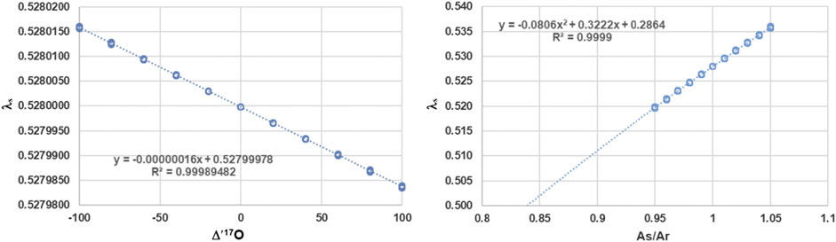
FIGURE 1. Left panel: Dependence of λ_s on ${{\Delta }^{\prime }}^{17}O$. The slightly blurred open circles toward more negative and more positive values corresponds to the ${{\displaystyle {}^{18}R}}_s$. Right panel: Dependence of λ on ratio A_s/A_r. The slightly blurred open circles in both panels correspond to the other dependences of ${{\Delta }^{\prime }}^{17}O$ and ${{\displaystyle {}^{18}R}}_s$ in the range of [-100,100] per meg or per mil, respectively. The dashed lines correspond to regressions (linear or quadratic) of the dependencies given with corresponding equations and R².

However, as shown by Kaiser (Kaiser, 2008) one has to consider not only the value of λ, but also the proportionality constant A which might be different for the sample and reference. Hence Eq. 9 must be replaced by Eq. 10, which is the general dependence of λ on the sample and reference system.

${\lambda }_s=\frac{\ln \left(1+{{\Delta }^{\prime }}^{17}O\right)-\ln \left(A_s/A_r\right)}{\ln \left({{\displaystyle {}^{18}R}}_s\right)}+\mathrm{0.528.}(10)$

The right panel of Figure 1 clearly documents that the most important dependence by far is the ratio of the proportionality constants. λ_s of Eq. 10 becomes 0.528 when ${{\Delta }^{\prime }}^{17}O$ equals zero and A_s equals A_r, the system that is generally applied. The question, however, remains whether this assumptions that led to this system are indeed valid.

Results

Two Component Mixing

Assuming a two component mixing of two water standards with known values (δ¹⁷O, δ¹⁸O, Δ¹⁷O), then we can write following Eq. 3:

$\Delta {}_1{}^{17}O=\ln \left({\delta }_1^{17}+1\right)-0.528\cdot \ln \left({\delta }_1^{18}+1\right),(11)$

$\Delta {}_2{}^{17}O=\ln \left({\delta }_2^{17}+1\right)-0.528\cdot \ln \left({\delta }_2^{18}+1\right).(12)$

The question arises what happens when we look into a mixture of these two waters, i.e. x_m times standard water 1 and (1 − x_m) times standard water 2 with x_m being a value between 0 and 1. Mathematically, it is clear that the mixed value of the primary delta values (δ¹⁷O, δ¹⁸O) are scaling linearly with the mixing value x_m. This leads to:

${\delta }_m^{17}=x_m\cdot {\delta }_1^{17}+\left(1-x_m\right)\cdot {\delta }_2^{17},(13)$

${\delta }_m^{18}=x_m\cdot {\delta }_1^{18}+\left(1-x_m\right)\cdot {\delta }_2^{18}.(14)$

And hence

$\begin{array}{l}\Delta {}_m{}^{17}O=\ln \left({\delta }_m^{17}+1\right)-0.528\cdot \ln \left({\delta }_m^{18}+1\right)\\ =\ln \left(x_m\cdot {\delta }_1^{17}+\left(1-x_m\right)\cdot {\delta }_2^{17}+1\right)-0.528\cdot \ln \left(x_m\cdot {\delta }_1^{18}+\left(1-x_m\right)\cdot {\delta }_2^{18}+1\right).\end{array}(15)$

The question that arises is whether Eq. 15 is equivalent to Eq. 16?

${\Delta }^{″}{}_m{}^{17}O=x_m\cdot \Delta {}_1{}^{17}O+\left(1-x_m\right)\cdot \Delta {}_2{}^{17}O.(16)$

For the two end points, i.e. $x_m$ = 0 or 1, the two Eqs. 15, 16 are equivalent, which can easily be checked by introducing these $x_m$ values into these two equations and considering Eqs. 9, 10. It is slightly more difficult for the other $x_m$ values in its given range. It can be checked either purely mathematically but also experimentally. First, mathematically it can be shown, using again a Taylor expansion, that they are different for different δ¹⁸O values. The difference is highest when $x_m$ equals 0.5, i.e. a mixture of 50% of each standard water.

Second, we have also done it experimentally in our lab with three standard waters (Bern_Slap (BS), Bern_DomeC (DC), Meerwasser (MW)) that are different in their Δ¹⁷O values, and one was different in its δ¹⁸O values from the other two. We performed mixtures of these standards in 10% steps. For each of the different mixed samples we performed 10 consecutive injections, corresponding to colored dots in Figure 2. We used two additional standards for calibration purposes, namely ST-08 (ST) and Eiswasser (EW). The measurement sequence for series 1 and 2 was setup as follows: Measurement number 1–10 corresponds to MW, 11–20 to ST, 21–30 to EW, 31–50 to BS, 51–60–90% BS +10% DC, 61–70–80% BS + 20% DC, ⋯⋯141–150 to DC, 151–160 to MW, 161–170 to ST, 171–180 to EW and 181–190 BS. A similar setup was made for series 3 and 4 but DC was exchanged with MW.

FIGURE 2

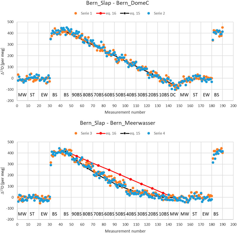
FIGURE 2. Upper panel, mixing series (1 and 2) in steps of 10% of two standard water with different Δ¹⁷O but similar δ¹⁸O values, i.e. Bern_Slap, BS (412 per meg, -55.21 per mil) and Bern_DomeC, DC (−54 per meg, −54.18 per mil). Lower panel: Mixing series (3 and 4) in steps of 10% of two standard water with different Δ¹⁷O as well as different δ¹⁸O values, i.e. Bern_Slap, BS (412 per meg, −55.21 per mil) and Meerwasser, MW (−3 per meg, −0.043 per mil). Δ¹⁷O is calculated based on Eq. 4. ST (ST-08) and EW (Eiswasser) correspond to two additional standards for calibration purposes. The number before BS need to be read as, e.g. 90 BS stands for 90% BS and 10% DC (series 1 and 2) or MW (series 3 and 4), respectively.

It clearly documents the dependence of the Δ¹⁷O on δ¹⁸O value. Differences shown are in the order of 100 per meg for a difference of 55 per mil for δ¹⁸O. This is the result of the definition of Δ¹⁷O based on the logarithmic difference of scaled oxygen isotope ratios according to Eq. 4. In agreement with the theory the maximal difference is reached for a 50%–50% mixture. The results does also not change significantly when using Eq. 5. Differences between the two definitions for Δ¹⁷O, i.e. Eq. 4 or Eq. 5, do only matter when the relationship between oxygen isotopes deviates significantly from the used power law with exponent 0.528 described in Eq. 1. This is the case for instance for stratospheric samples for which the exponent is near 1 rather than 0.5. For those samples differences between the two definitions can amount up to several 100 per meg.

Mixing of Kinetic and Equilibrium Fractionation

Regarding the water cycle combinations of kinetic and equilibrium fractionations during evaporation, evapo-transpiration and condensation are inherent.

Therefore, the overall fractionation is a combination of the kinetic, ${\alpha }_{\text{kin}}$, and equilibrium ${\alpha }_{\text{eq}}$, fractionation.

${\alpha }_{\text{tot}}^i\left(T,h,n\right)={\alpha }_{\text{kin}}^i\left(h,n\right)\cdot {\alpha }_{\text{eq}}^i\left(T\right).(17)$

The equilibrium fractionation between liquid water and water vapor that we have used here are from Ellhoj (Ellehoj et al., 2013) for T below the freezing point and Horita and Wesolowski (Horita and Wesolowski, 1994) above it. The kinetic fractionation relates to water molecule diffusion in the vapor phase in air and is a function of the prevailing relative humidity, h, $D_{i,\text{air}}$ and a turbulence factor n (Barkan and Luz, 2007).

${\alpha }_{\text{kin}}^i\left(h,n\right)=h+\left(1-h\right)\cdot {\left(\frac{D_{\text{HHO},\text{air}}}{D_{i,\text{air}}}\right)}^n,(18)$

where $D_{i,\text{air}}$ corresponds to the diffusion coefficient of the water isotopologues (vapor phase) in air, i.e. i denotes either HH¹⁷O, HH¹⁸O, or HD¹⁶O. It has been shown that the equilibration and kinetic fractionation between H₂¹⁷O and H₂¹⁸O scales with an exponent λ_eq = 0.529 (Barkan and Luz, 2005) and λ_kin = 0.518 (Barkan and Luz, 2007).

Figure 3 values corresponds to a combination of Eq. 17 for two cases, 1) for h = 1 corresponding to the equilibrium fractionation only and 2) the common case of Eq. 17. The balance value x corresponds here to:

$\left(1-x\right)\cdot {\alpha }_{\text{eq}}+x\cdot {\alpha }_{\text{kin}}\cdot {\alpha }_{\text{eq}}.$

FIGURE 3

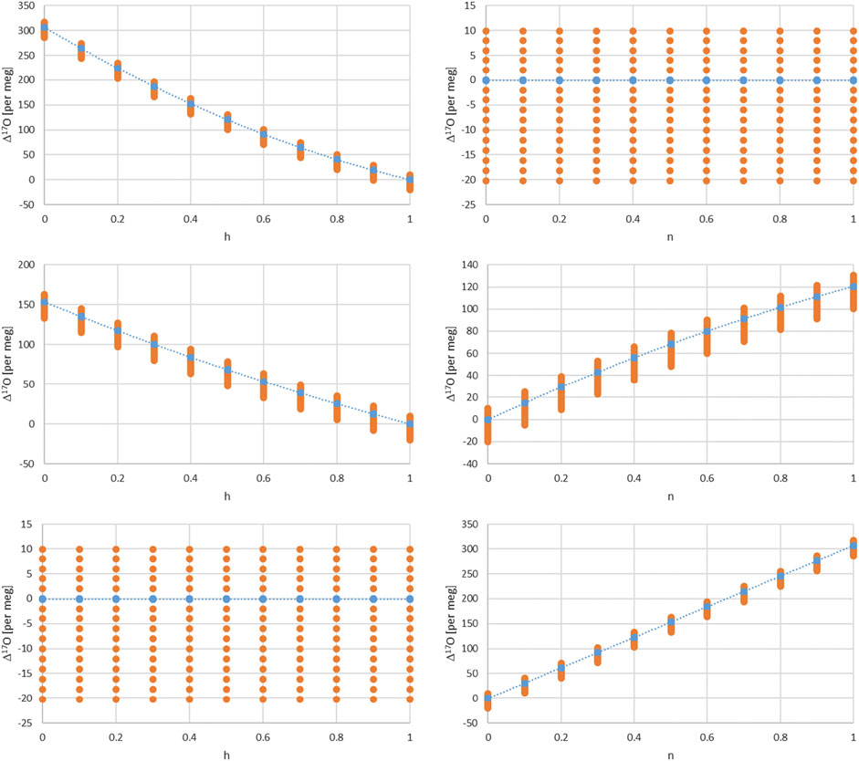
FIGURE 3. Dependence of Δ¹⁷O on the relative humidity h for different turbulence factors of 1, 0.5, and 0 (upper, middle and lower left panels). Dependence of Δ¹⁷O on the turbulence factor n for different relative humidity values of 1, 0.5 and 0 (upper, middle and lower right panels). The dots corresponds to δ18O values from −20 to 10 per mil in steps of 2 and therefore indirectly to a temperature range shown in Figure 4.

FIGURE 4

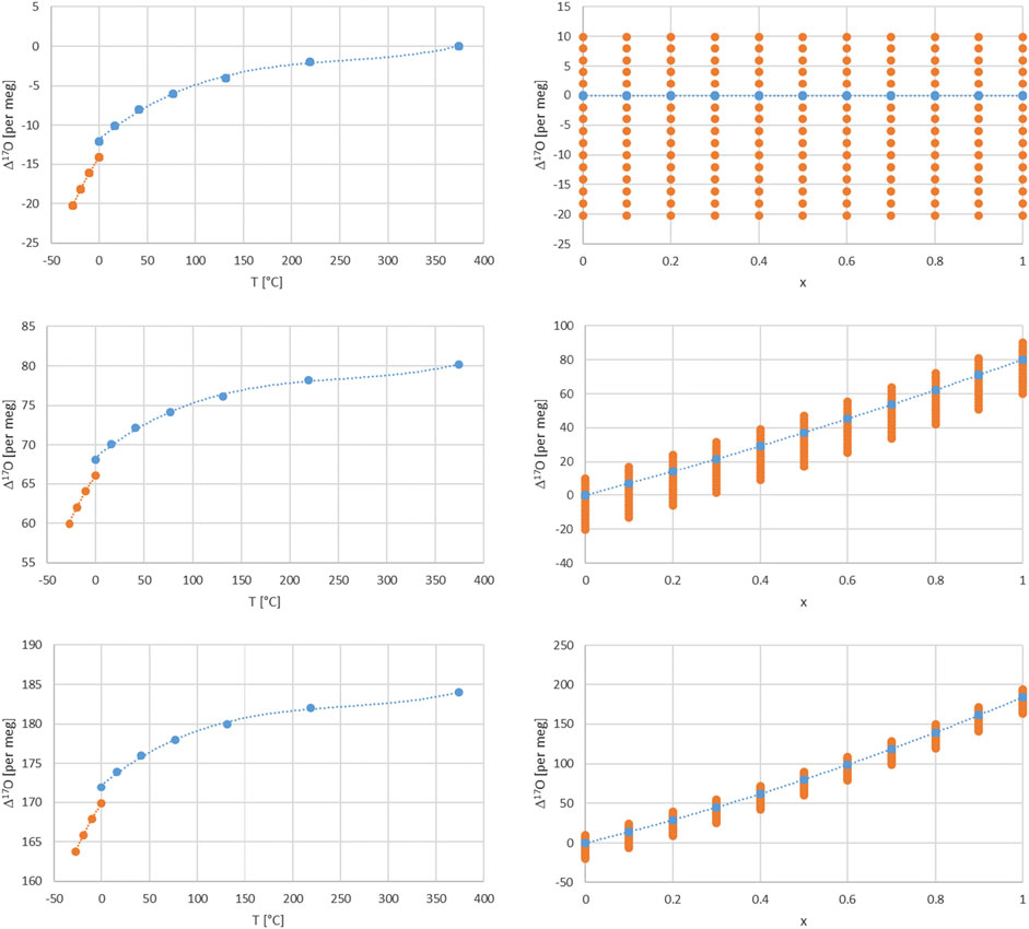
FIGURE 4. Dependence of Δ¹⁷O on temperature for a turbulence factor n of 0.6, x = 1 and for different relative humidity values of 1, 0.5, and 0 (upper, middle and lower left panels). Orange dashed line for fractionation values between ice and vapor (Ellehoj et al., 2013) and blue dashed line for fractionation values between liquid and vapor water phase (Horita and Wesolowski, 1994). Dependence of Δ¹⁷O on the balance factor x for a turbulence factor n of 0.6 for different relative humidity values of 1, 0.5, and 0 (upper, middle and lower right panels). The dots correspond to δ¹⁸O values from −20 to 10 per mil in steps of 2.

It corresponds to real situations such as mixing of water vapor that is in equilibrium with the liquid phase (case 1) with water vapor that is additionally exposed to kinetic fractionation (case 2).

There are several dependencies when combining the kinetic and equilibrium fractionation. We first look into the relative humidity and turbulence factor dependence by choosing three values for their respective range, i.e. 0, 0.5 and 1 (Figure 3). Regarding humidity, these values corresponds to completely dry conditions (h = 0) with strong kinetic fractionation contribution to the total fractionation, Eqs. 17, 18. For wet conditions (h = 1) kinetic fractionation is absent according to Eq. 18, and for 50% humidity (h = 0.5) which corresponds to an interplay of kinetic and equilibrium fractionation. Similarly, regarding turbulence, they correspond to completely turbulent conditions (n = 0) which corresponds to no diffusion influence in contrast to pure molecular diffusion (n = 1) or intermediate, mixed conditions (n = 0.5) between pure molecular and turbulent diffusion. The temperature dependence is indirectly shown by the orange dots via the corresponding δ¹⁸O value dependence. It ranges from −20 to +10 per mil in these plots. A direct temperature dependence is given in Figure 4 and corresponds to an extended temperature range compared to the range of meteoric waters.

Furthermore, one can consider air masses with water vapor of different origin to be mixed. In this case an additional parameter comes into play, i.e. the balance between these air masses and corresponding water vapor contents and isotope compositions. The simplest case is a mixture of two air masses which can be characterized by a balance value x in the range of 0–1 as shown above. Assuming that one water vapor is in complete equilibrium (h = 1) and the other experienced kinetic fractionation (h = 0 or 0.5) in addition with an intermediate turbulence factor n = 0.6 and additionally for different δ¹⁸O values leads to the dependence of Δ¹⁷O on x shown in Figure 4. Similarly the direct influence of temperature is given in Figure 4 for n = 0.6 and dry, intermediate and humid conditions h= (0, 0.5, 1).

In order to shed light on the relevance of their weighting functions we can have a look at data obtained on selected sites within the Swiss network for precipitation (ISOT), see Materials and Methods. To further investigate these fractionation behavior under real conditions, Disentangling Kinetic from Equilibrium Fractionation, we use our measurements on seven stations.

Disentangling Kinetic From Equilibrium Fractionation

Fractionation occurs at the source where the water vapor is produced, on its path to the site and at the site itself. Generally, these fractionations are combinations of kinetic associated with diffusion of water molecules in the vapor phase in air and equilibrium fractionations associated with phase changes. Additionally, as discussed above air masses of different origins containing different vapor water contents with potentially different isotope ratios could mix. A way of summarizing these different fractionations in a simplified approach is often done by the so-called Rayleigh model (Kendall and Caldwell, 1998) (Figure 5). It relates the isotope composition of precipitation to the corresponding source composition and mathematically it reads:

$R_s^i=R_0^i/{\alpha }_{\text{tot}}^{i,\text{source}}\cdot f^{\left({\alpha }_{\text{tot}}^{i,\text{path}}-1\right)}\cdot {\alpha }_{\text{tot}}^{i,\text{site}},(19)$

where f corresponds to the remaining water content that can be estimated based on the prevailing water saturation pressures that are themselves dependent on temperatures at the source and the site. $R_s^i$ and $R_0^i$ are the isotope ratios of liquid water at the site of precipitation and the source of water vapor production, respectively. $R_0^i$ corresponds to the isotope composition of the ocean water and will be taken as a reference here $R_0^i=R_r^i$. All fractionation factors show the dependences as given in Eqs. 17, 18. In our calculations we use a simplification of the fractionation along the path by using a weighted mean of the fractionations at the source and the site.

${\alpha }_{\text{tot}}^{i,\text{path}}\left(y\right)=y\cdot {\alpha }_{\text{tot}}^{i,\text{source}}+\left(1-y\right)\cdot {\alpha }_{\text{tot}}^{i,\text{site}}.(20)$

FIGURE 5

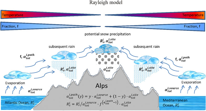
FIGURE 5. Conceptual scheme of a simple Rayleigh approach to characterize the source and site conditions using the seven Swiss precipitation sites. Fractionations at the source, along the air trajectory and at the site are included, all fractionations are subject to a combination of temperature dependent equilibrium fractionations and humidity and turbulence factor dependent kinetic fractionations.

This indirectly takes into account a re-evaporation mechanisms at the site where the precipitation takes place since it includes also the turbulence factor as well as the humidity factor at the site.

In order to investigate the validity and robustness of this simplified method, we compared the data derived values with the Rayleigh model estimates. For that we estimated the expected f values for seven stations in Switzerland. The characteristics of these stations are given in Table 1 and the results of our estimates are listed in Table 2.

TABLE 1

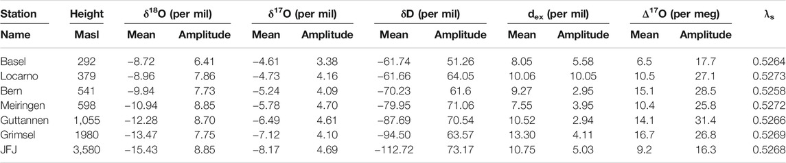
TABLE 1. Measured monthly means and monthly mean amplitudes for seven stations of the Swiss ISOT network. λ_s is calculated based on ln $\left(R_s^{17}/R_r^{17}\right)$ to ln $\left(R_s^{18}/R_r^{18}\right)$ plots.

TABLE 2

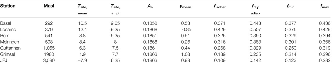
TABLE 2. Comparison of Rayleigh parameter f based on meteo data (f_isobar, f_{dry adiabatic}) vs. isotope data (pure source influenced, y = 1 → f_min or pure site influenced, y = 0 → f_max), y_mean is related to f_mean (mean of f_isobar and f_{dry adiab}), A_s is calculated based on Eq. 23 from A_r = 0.187,664,259 and λ_s from Table 1. For the dry adiabatic calculations we used a value κ = c_p/c_v of 1.4 for heat capacity of water at constant pressure (c_p) and constant volume (c_v).

In a more sophisticated approach one can use source conditions that are based on back-trajectory analyses for each individual station. This would be particularly important for the Locarno station since it is located south of the Alps whereas all other are in the center or north of the Alps. Furthermore, the fractionation associated with condensation based on the actual meteorological parameters including values along vertical falling path of precipitation.

Here, we used the same source conditions for all stations. The condition of the water vapor source was set to a mean annual temperature of 24°C with an amplitude (max–min) of 4°C and a relative humidity value of 94.7%. The site conditions are corresponding to mean annual temperatures and their corresponding amplitudes obtained from measured data from MeteoSwiss (Table 2) as well as a relative humidity value of 94%. The turbulence factor has been fixed for these calculations at 0.88 for the humidity source location and at 1 at the site of precipitation. Based on these values, fractionation factors were calculated following Eqs. 17, 18.

We used two different approaches an isobaric case with f values between 0.11 and 0.429 and a dry adiabatic case with values between 0.162 and 0.493. Dry adiabatic conditions lead to higher remaining water vapor contents. The ranges are characterized by the temperature dependence on altitude as expected and an observed Δ¹⁷O altitude dependence (Figure 6). These values can now be compared with the data derived range for f based on the maximal and minimal values for y, i.e. 1 (f_min) and 0 (f_max), estimated from Eq. 21. It was surprising how well the ranges agreed. Only Locarno and JFJ showed somewhat shifted ranges (Table 2; Figure 6). Lower enrichments for Locarno’s f values are observed that are derived from the isotope data compared to those derived from metadata. For JFJ the upper bound value is very different which is also seen but to a lesser extent for the second highest station Grimsel.

FIGURE 6

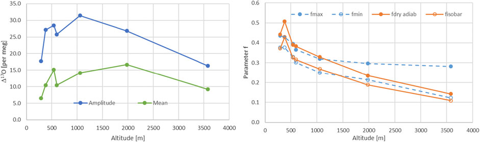
FIGURE 6. Left panel, mean and amplitude of Δ¹⁷O for all of the seven Swiss stations. Right panel, comparison of the f values of the Rayleigh model, corresponding to the remaining water content, calculated based on the stations metadata from MeteoSwiss (orange) for the isobaric and dry adiabatic case and the corresponding values based on maximal and minimal y-values (see text).

Using Eq. 1 for a sample (here precipitation at a specific site) and the reference (here water at the source location of the corresponding water vapor formation), one can combine it with Eq. 19 to

$\ln \left(R_s^{17}/R_r^{17}\right)=\ln \left(\frac{f^{\left({\alpha }_{\text{tot}}^{17,\text{path}}\left(y\right)-1\right)}\cdot {\alpha }_{\text{tot}}^{17,\text{site}}}{{\alpha }_{\text{tot}}^{17,\text{source}}}\right)=\ln \left(\frac{\left(A_s\cdot R_s^{18{\lambda }_s}\right)}{\left(A_r\cdot R_r^{18{\lambda }_r}\right)}\right).(21)$

Solving for y leads to

$y=\frac{\ln \left(A_s/A_r\right)+{\lambda }_s\cdot \ln \left(R_s^{18}\right)-{\lambda }_r\cdot \ln \left(R_r^{18}\right)+\ln \left({\alpha }_{\text{tot}}^{17,\text{source}}\right)-\ln \left({\alpha }_{\text{tot}}^{17,\text{site}}\right)+\ln \left(f\right)\cdot \left(1- {\alpha }_{\text{tot}}^{17,\text{site}}\right)}{\left({\alpha }_{\text{tot}}^{17,\text{source}}-{\alpha }_{\text{tot}}^{17,\text{site}}\right)\cdot \ln \left(f\right)},$

where $R_s^{18}$ is measured, the fractionation factors can be calculated from the above-mentioned references and the prevailing humidity and turbulence factor n (see discussion below), ${\lambda }_s$ corresponds to the slope when regressing ln ($R_s^{17}/R_r^{17}$) as y-axis to ln ($R_s^{18}/R_r^{18}$) as x-axis, A_s and A_r corresponds to the proportionality constants for the sample and the reference, respectively. A_r is given whereas A_s can also be calculated from the intercept b of the above regression and by using Eq. 1, it corresponds to

$A_s=e^b\cdot A_r\cdot R_r^{18{\lambda }_r-{\lambda }_s}(23)$

Furthermore, we optimized the parameter n, h for the source and site, and the balance of contribution between these, i.e. y, by minimizing the sum of squared differences of measured and modeled monthly means as well as squared differences between monthly measured and modeled mean monthly amplitudes of the individual station’s precipitation isotope signature. The optimization was done with an iterative Generalized Reduced Gradient solver approach using non-linear engine. We performed calculations with multiple initial conditions to enhance the chance to find the global minimum. This led to the values for n, h, and y given in Table 3. The comparison between the data and modeled values are given in Figures 7–13.

TABLE 3

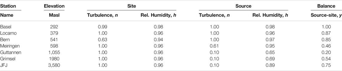
TABLE 3. Source and site conditions optimized by minimizing squared differences of measured and modeled monthly mean isotope ratios and corresponding amplitudes as given in Table 1.

FIGURE 7

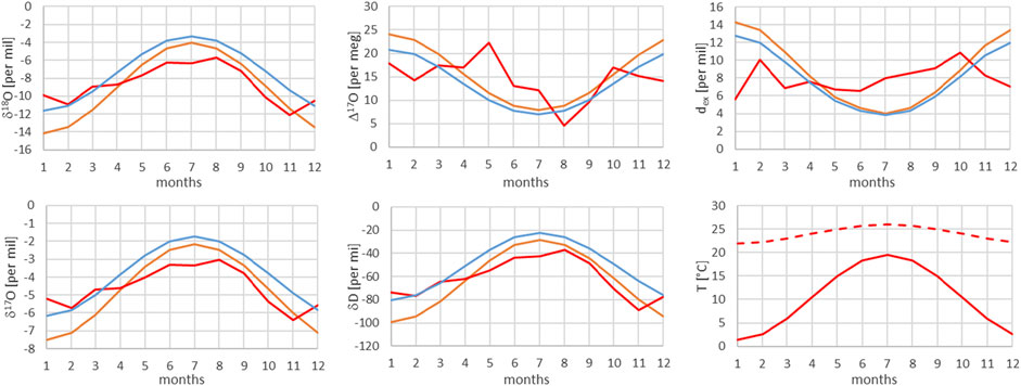
FIGURE 7. Comparison of monthly mean measured (red) and modeled (for the isobaric case (orange) and for the dry adiabatic case (blue)) isotope ratios for Basel. The dashed red line corresponds to the assumed source temperature.

FIGURE 8

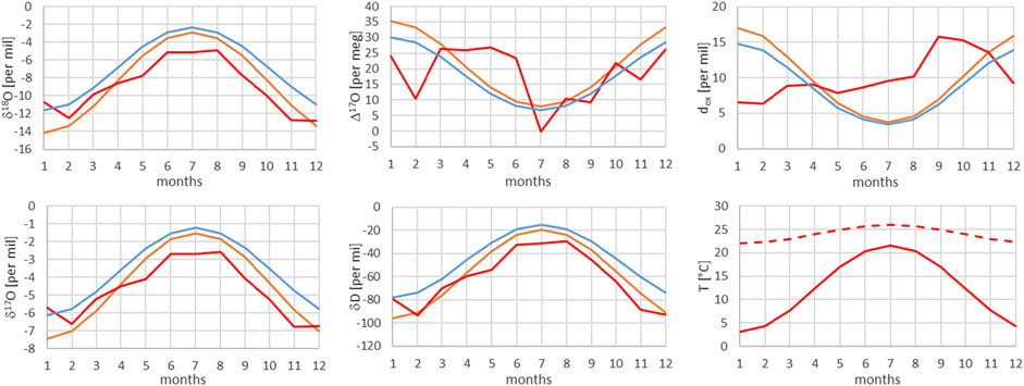
FIGURE 8. Comparison of monthly mean measured (red) and modeled (for the isobaric case (orange) and for the dry adiabatic case (blue)) isotope ratios for Locarno. The dashed red line corresponds to the assumed source temperature.

FIGURE 9

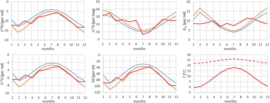
FIGURE 9. Comparison of monthly mean measured (red) and modeled (for the isobaric case (orange) and for the dry adiabatic case (blue)) isotope ratios for Bern. The dashed red line corresponds to the assumed source temperature.

FIGURE 10

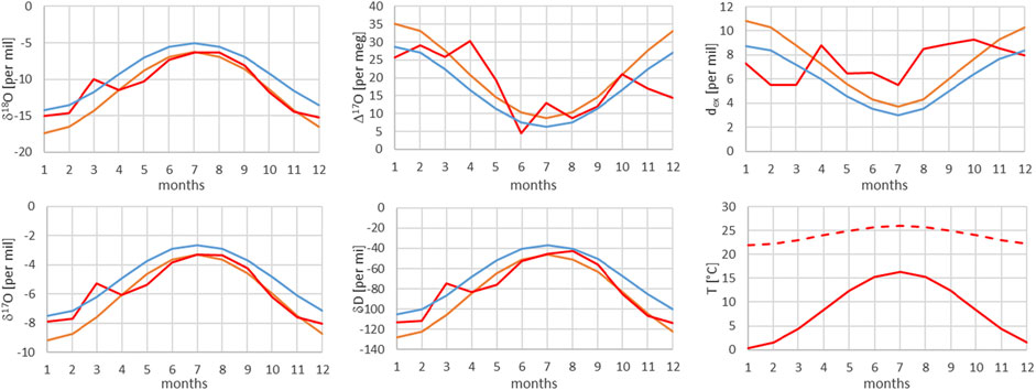
FIGURE 10. Comparison of monthly mean measured (red) and modeled (for the isobaric case (orange) and for the dry adiabatic case (blue)) isotope ratios for Meiringen. The dashed red line corresponds to the assumed source temperature.

FIGURE 11

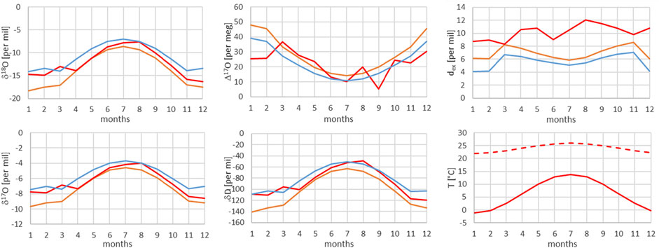
FIGURE 11. Comparison of measured (red) and modeled (for the isobaric case (orange) and for the dry adiabatic case (blue)) isotope ratios for Guttannen. The dashed red line corresponds to the assumed source temperature.

FIGURE 12

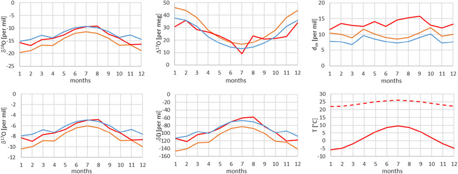
FIGURE 12. Comparison of monthly mean measured (red) and modeled (for the isobaric case (orange) and for the dry adiabatic case (blue)) isotope ratios for Grimsel. The dashed red line corresponds to the assumed source temperature.

FIGURE 13

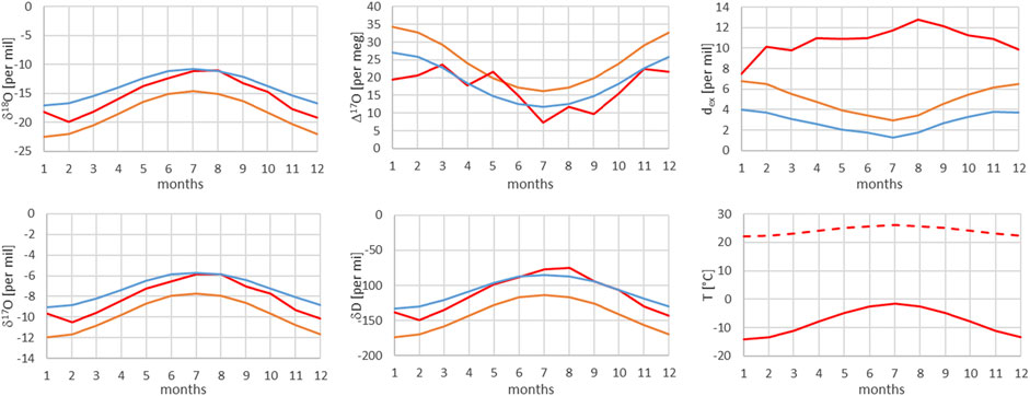
FIGURE 13. Comparison of monthly mean measured (red) and modeled (for the isobaric case (orange) and for the dry adiabatic case (blue)) isotope ratios for Jungfraujoch (JFJ). The dashed red line corresponds to the assumed source temperature.

Discussion

The expected dependence of Δ¹⁷O on δ¹⁸O based on the definition of Δ¹⁷O was proven by a two water standard mixing experiment. The primary delta value scale linearly with the mixing ratio whereas the Δ¹⁷O is dependent on the mixing ratio as well as on the δ¹⁸O. However, it also shows that if the δ¹⁸O is equal or similar, Δ¹⁷O scales linearly with the mixing ratio. We intentionally performed these experiments to show that one has to pay attention when mixing two waters in order to come up with a range of standards for high precision ¹⁷O measurements. δ¹⁷O and δ¹⁸O will be linearly scaling with the mixing ratio of these waters but not necessarily the mixed Δ¹⁷O. This is of particular interest since one can derive Δ¹⁷O with higher precision than the δ¹⁷O due to cancellation of variations in both oxygen isotope ratios.

Dependencies of Δ¹⁷O on relative humidity, turbulence factor, temperature as shown in Figure 3, 4 have also been investigated previously experimentally as well as theoretically (Landais et al., 2010; Gibson et al., 2016; Surma et al., 2018; Uechi and Uemura, 2019). Regarding relative humidity, different results were obtained from correlation analysis of Δ¹⁷O with primary isotopes (δ¹⁷O and δ¹⁸O), i.e. either a positive (Uechi and Uemura, 2019) or a negative dependence (Landais et al., 2010), yet in significantly different environments (high and low relative humidity conditions). In both studies convincing theoretical considerations are given, how the measured Δ¹⁷O values can be explained in which the relative humidity plays a key role. In tropical and subtropical regions Δ¹⁷O values is a measure for the relative humidity of the oceanic moisture source region (Uechi and Uemura, 2019) whereas over land the relative humidity among other is a driver for re-evaporation processes as discussed in Landais et al., (Landais et al., 2010). These two studies exemplarily show how different the influences on the water stable isotope composition can be, particularly when strongly divergent relative humidity conditions are compared. Additionally to the humidity condition the amount effect comes into play for which the slope between the primary isotopes (δ¹⁷O and δ¹⁸O) as discussed in (Uechi and Uemura, 2019) are critical for the interpretation of Δ¹⁷O values shown in (Landais et al., 2010). Regarding our measurements of the Swiss precipitation sites, measured relative humidity exhibits intermediate to high observed values in the range of 50%–95%. Therefore, we would not expect a strong effect of re-evaporation, however we cannot exclude it for specific individual rain events during low humidity conditions. Furthermore, the modeled relative humidity values are in the range of their observed values.

The dependencies of Δ¹⁷O on the turbulence factor as shown in Figure 3 are opposite to the relative humidity conditions, i.e. the higher the turbulence factor the higher the change in Δ¹⁷O. The dependence of turbulence have been discussed in several previous publications (Merlivat, 1978; Horita et al., 2008). Specific studies investigated its influence on Δ¹⁷O of surface water in arid zones (Surma et al., 2018) or on lake water (Gibson et al., 2016). A turbulent value, n = 1, corresponding to completely stagnant conditions, i.e. soil water or water in plant leaves, leads to fully developed diffusional conditions and therefore to maximal kinetic fractionation for the prevailing humidity value. In contrast, a turbulence value of zero corresponds to fully turbulent conditions with absent kinetic fractionation independent on prevailing humidity conditions. More information regarding the turbulence conditions for the Swiss precipitation sites is given below.

Regarding disentangling kinetic from equilibrium fractionation from measurements performed within the Swiss network of isotopes on precipitation (ISOT), we proved that the simple Rayleigh approach yields the correct range of water vapor fractions remaining at the site of condensation. Additionally, it also documents the seen anti-correlation between Δ¹⁷O and δ¹⁷O, δ¹⁸O, and δD. This means that there seems to be limited admixture influence of completely different water isotope signatures, e.g. re-evaporated water on land or from lakes. Furthermore from the log-log plots, we derived the exponents for the relationship between δ¹⁷O and δ¹⁸O for all sites. All these values are below 0.529, corresponding to the equilibrium fractionation exponent, which first tells us that there is most probably a combination of kinetic and equilibrium fractionation at action to form the precipitation. Yet, as nicely documented by Passey and Levin (Passey and Levin, 2021) a lower slope than 0.529 (equilibration fractionation) on meteoric waters does not necessarily mean that a combination of equilibrium and kinetic fractionation is needed due to the sequential rain out along the path.

The balance between the source and the site signature influence is crucial to understand what drives the isotopic precipitation signal. This balance of influence has been studied with our stations in Switzerland giving access to a north south transect as well as an altitude range. From the experiment, we see that for lower elevated sites the source signature is more important compared to the higher elevated sites. Minimal source influence has been found for intermediate altitudes, i.e. Guttannen and Grimsel stations (Table 3). The altitude dependence for Δ¹⁷O shown in Figure 5 documents the highest values for these intermediate sites. A negative correlation is therefore obtained between Δ¹⁷O and the source-site balance values y. This points to an influence from both the source as well as from the site conditions on Δ¹⁷O. Relative humidity together with the turbulence parameter are the driving forces for the water stable isotope fractionation at both the formation location of the humidity as well as at the site of precipitation. Optimization of the turbulence factor and relative humidity at the source and site lead to moderate variations for the relative humidity at the source of 0.65–0.98 whereas it is strongly restricted to small range close to unity for the relative humidity at the site (0.94–0.98). This indicates that re-evaporation after precipitation formation according (Uechi and Uemura, 2019) is strongly limited and therefore the type of precipitation formation (snow or rain) might be of minor influence. Yet, further studies are necessary in particular due to the fact that the seasonal dependence of d_ex values are not well matched at all.

In contrast, the turbulence factor values use the complete range (0.1–1) for the source of water vapor whereas it is limited to higher values (0.63–1) for the precipitation site. The latter is favoring kinetic fractionation whereas the high relative humidity at the site hinders it. Since relative humidity and the turbulence factor have opposite influences on Δ¹⁷O (Mixing of Kinetic and Equilibrium Fractionation), it might be an artifact of the optimizing routine that leads to the full range in n for the water vapor source location or due to the simple model approach as presented here. In literature a value of 0.6 for n is often used (Merlivat and Jouzel, 1979) to account for the influence of turbulent conditions prevailing at an evaporation site. Yet, there are contrasting studies regarding the value of n. A recent publication indicates that a value near 1 should be favored (Bonne et al., 2019) based on many direct observation. Another recent publication (Gonfiantini et al., 2020) documents laboratory experiments resulting in a strong wind dependence with values similar as generally assumed with 0.5 for windless conditions and lower values with increasing wind velocities. Yet, the authors reported that the values for δD and δ¹⁸O are deviating the higher the applied wind speed (up to 2.5 m/s) gets. In summary, the whole range seems to be plausible.

The optimization lead to an improvement of the balance value y which reaches values within its expected range between 0 and 1. This is also the case of the humidity values which are close to unity for the site of precipitation and lower for source locations of three precipitation sites, namely Guttannen, Grimsel and Jungfraujoch. These stations also have rather unrealistically low turbulence factors. This might indicate that our assumption of the same conditions for the humidity source for all seven sites is not valid. As we know from other studies, sites north of the Alps are mainly governed by North Atlantic sea sources whereas those south of the Alps from the Mediterranean sea. Further studies are required to account for this Alpine barrier for air circulation and its influence on precipitation isotopes.

From Figures 7–13, it can be learnt that the agreement for the primary stable isotope ratios δ¹⁷O, δ¹⁸O and δD is very good. Regarding the secondary parameters, Δ¹⁷O is in much better agreement than d_ex. Since Δ¹⁷O is significantly less temperature dependent than d_ex it might point to a temperature influence that has not been taken into account yet. Here, one can think of temperature differences between condensation and site temperatures. This has to do with the mean cloud height above lowlands and the Alpine area. Most certainly the temperature difference between condensation and site temperatures is higher for lower altitude sites. Additional studies are required to further shed light on this issue.

Conclusion

We demonstrated the non-linear dependence of Δ¹⁷O in contrast to the linear dependencies of δ¹⁸O and δ¹⁷O when water mixing is applied. We proved this experimentally by measuring three laboratory internal water standards with significantly different Δ¹⁷O and δ¹⁸O values. It is important that the primary isotope ratios scales linearly in contrast to Δ¹⁷O which show a higher order dependence as expected from its definition. A simple Rayleigh model approach yields to a rather good agreement for four out of the five isotope parameters for each of the seven stations with the exception of d_ex. It documents a clear interplay of kinetic with equilibrium fractionation. It has been noticed that the contribution of source and site on the corresponding fractionation is important to match the measurements. The source signal contribution is more important for lower than higher elevated sites and least important for intermediate heights. The turbulence factor is difficult to judge since the complete range from zero to unity has been obtained when matching the data with minimal deviations. In contrast, humidity could be rather well determined. This somewhat inconclusive results might be due to our assumption of similar conditions for all seven stations since they are situation on a north-south transect through the Alps exhibiting different source locations, i.e. North Atlantic and the Mediterranean sea and are situated at different altitudes.

Data Availability Statement

The raw data supporting the conclusions of this article will be made available by the authors, without undue reservation.

Author Contributions

ML has designed the study. SR has performed the measurements. ML wrote the manuscript with help from SR.

Funding

This work was supported by the EU-funded project INitial TRAining network on Mass Independent Fractionation (Intramif) as well as the Swiss National Science Foundation (SNF-125116 and SNF- 135152).

Conflict of Interest

The authors declare that the research was conducted in the absence of any commercial or financial relationships that could be construed as a potential conflict of interest.

Acknowledgments

The authors would like to acknowledge the Federal Office for the Environment for their support in maintaining the Swiss network for isotope on precipitation (ISOT). Thanks goes to MeteoSwiss for providing meteorological parameter data and all persons taking the samples at different locations involved in this study. We would like to thank the International Foundation High Altitude Research Stations Jungfraujoch and Gornergrat for allowing to perform the water sampling at Jungfraujoch. We would like to express thanks for the mechanical and electronic workshop staff at the Division of Climate and Environmental Physics Division. Peter Nyfeler assisted in the laboratory and gave advice in technical issues and took care of the water sampling. Hanspeter Moret took care of water sampling at the University of Bern and was responsible for the development and maintenance of electronic devices. We very much appreciate the reviewer’s and editor’s comments that led to a significant improvement of the manuscript.

References

Aemisegger, F., Pfahl, S., Sodemann, H., Lehner, I., Seneviratne, S. I., and Wernli, H. (2014). Deuterium excess as a proxy for continental moisture recycling and plant transpiration. Atmos. Chem. Phys. 14, 4029–4054. doi:10.5194/acp-14-4029-2014

CrossRef Full Text | Google Scholar

Affolter, S., Häuselmann, A. D., Fleitmann, D., Häuselmann, P., and Leuenberger, M. (2015). Triple isotope (δD, δ17O, δ18O) study on precipitation, drip water and speleothem fluid inclusions for a Western Central European cave (NW Switzerland). Quat. Sci. Rev. 127, 73–89. doi:10.1016/j.quascirev.2015.08.030

CrossRef Full Text | Google Scholar

Aggarwal, P. K., Froehlich, K. F., and Gat, J. R. (2005). Isotopes in the water cycle. Berlin, Germany: Springer.

Allen, S. T., Keim, R. F., Barnard, H. R., Mcdonnell, J. J., and Renée Brooks, J. (2017). The role of stable isotopes in understanding rainfall interception processes: a review. WIREs Water. 4, e1187. doi:10.1002/wat2.1187

CrossRef Full Text | Google Scholar

Andrews, J. E. (2006). Palaeoclimatic records from stable isotopes in riverine tufas: synthesis and review. Earth-Science Rev. 75, 85–104. doi:10.1016/j.earscirev.2005.08.002

CrossRef Full Text | Google Scholar

Angert, A., Cappa, C. D., and Depaolo, D. J. (2004). Kinetic 17O effects in the hydrologic cycle: indirect evidence and implications. Geochimica et Cosmochimica Acta. 68, 3487–3495. doi:10.1016/j.gca.2004.02.010

CrossRef Full Text | Google Scholar

Assonov, S. S., and Brenninkmeijer, C. A. (2003). On the 17O correction for CO2 mass spectrometric isotopic analysis. Rapid Commun. Mass. Spectrom. 17, 1007–1016. doi:10.1002/rcm.1012

PubMed Abstract | CrossRef Full Text | Google Scholar

Aston, F. W. (1942). Mass spectra and isotopes. London, United Kingdom: Edward Arnold London.

Barkan, E., and Luz, B. (2007). Diffusivity fractionations of H2(16)O/H2(17)O and H2(16)O/H2(18)O in air and their implications for isotope hydrology. Rapid Commun. Mass. Spectrom. 21, 2999–3005. doi:10.1002/rcm.3180

PubMed Abstract | CrossRef Full Text | Google Scholar

Barkan, E., and Luz, B. (2005). High precision measurements of 17O/16O and 18O/16O ratios in H2O. Rapid Commun. Mass. Spectrom. 19, 3737–3742. doi:10.1002/rcm.2250

PubMed Abstract | CrossRef Full Text | Google Scholar

Barkan, E., Musan, I., and Luz, B. (2015). High-precision measurements of δ(17)O and (17) oexcess of NBS19 and NBS18. Rapid Commun. Mass. Spectrom. 29, 2219–2224. doi:10.1002/rcm.7378

PubMed Abstract | CrossRef Full Text | Google Scholar

Bird, M. I., and Ascough, P. L. (2012). Isotopes in pyrogenic carbon: a review. Org. Geochem. 42, 1529–1539. doi:10.1016/j.orggeochem.2010.09.005

CrossRef Full Text | Google Scholar

Bonne, J. L., Behrens, M., Meyer, H., Kipfstuhl, S., Rabe, B., Schönicke, L., et al. (2019). Resolving the controls of water vapour isotopes in the Atlantic sector. Nat. Commun. 10, 1632–1710. doi:10.1038/s41467-019-09242-6

PubMed Abstract | CrossRef Full Text | Google Scholar

Cernusak, L. A., Barbour, M. M., Arndt, S. K., Cheesman, A. W., English, N. B., Feild, T. S., et al. (2016). Stable isotopes in leaf water of terrestrial plants. Plant Cel Environ. 39, 1087–1102. doi:10.1111/pce.12703

CrossRef Full Text | Google Scholar

Chinard, F. P., and Enns, T. (1953). Preparation of water samples for deuterium analysis in mass spectrometer. Anal. Chem. 25, 1413–1414. doi:10.1021/ac60081a035

CrossRef Full Text | Google Scholar

Den Boer, D. H. W., and Borg, W. a. J. (1952). Mass spectrometric determination of deuterium in organic compounds. Recueil des Travaux Chimiques des Pays-Bas. 71, 120–124. doi:10.1002/recl.19520710203

CrossRef Full Text | Google Scholar

Dibeler, V. H. (1954). Mass spectrometry. Anal. Chem. 26, 58–65. doi:10.1021/ac60085a011

CrossRef Full Text | Google Scholar

Diefendorf, A. F., and Freimuth, E. J. (2017). Extracting the most from terrestrial plant-derived n-alkyl lipids and their carbon isotopes from the sedimentary record: a review. Org. Geochem. 103, 1–21. doi:10.1016/j.orggeochem.2016.10.016

CrossRef Full Text | Google Scholar

Dostrovsky, I., and Klein, F. (1952). Mass spectrometric determination of oxygen in water samples. Anal. Chem. 24, 414–415. doi:10.1021/ac60062a042

CrossRef Full Text | Google Scholar

Dubbs, C. A. (1953). Determination of deuterium. Anal. Chem. 25, 828–829. doi:10.1021/ac60077a052

CrossRef Full Text | Google Scholar

Ellehoj, M., Steen-Larsen, H. C., Johnsen, S. J., and Madsen, M. B. (2013). Ice-vapor equilibrium fractionation factor of hydrogen and oxygen isotopes: experimental investigations and implications for stable water isotope studies. Rapid Commun. Mass. Spectrom. 27, 2149–2158. doi:10.1002/rcm.6668

PubMed Abstract | CrossRef Full Text | Google Scholar

Epstein, S., Buchsbaum, R., Lowenstam, H., and Urey, H. C. (1951). Carbonate-water isotopic temperature scale. Geol. Soc. America Bull. 62, 417–426. doi:10.1130/0016-7606(1951)62[417:cits]2.0.co;2

CrossRef Full Text | Google Scholar

Friedman, L., and Irsa, A. P. (1952). Determination of deuterium in water. Anal. Chem. 24, 876–878. doi:10.1021/ac60065a031

CrossRef Full Text | Google Scholar

Galewsky, J., Steen-Larsen, H. C., Field, R. D., Worden, J., Risi, C., and Schneider, M. (2016). Stable isotopes in atmospheric water vapor and applications to the hydrologic cycle. Rev. Geophys. 54, 809–865. doi:10.1002/2015rg000512

PubMed Abstract | CrossRef Full Text | Google Scholar

Gibson, J. J., Birks, S. J., and Yi, Y. (2016). Stable isotope mass balance of lakes: a contemporary perspective. Quat. Sci. Rev. 131, 316–328. doi:10.1016/j.quascirev.2015.04.013

CrossRef Full Text | Google Scholar

Gonfiantini, R., Wassenaar, L. I., and Araguas‐Araguas, L. (2020). Stable isotope fractionations in the evaporation of water: the wind effect. Hydrological Process. 34 (16), 3596–3607. doi:10.1002/hyp.13804

CrossRef Full Text | Google Scholar

Graff, J., and Rittenberg, D. (1952). Microdetermination of deuterium in organic compounds. Anal. Chem. 24, 878–881. doi:10.1021/ac60065a032

CrossRef Full Text | Google Scholar

Griffiths, H. (1998). Stable isotopes: integration of biological, ecological and geochemical processes. Oxford, United Kingdom: Environmental Plant Biology Series. Bios, 303–321.

Horita, J., Rozanski, K., and Cohen, S. (2008). Isotope effects in the evaporation of water: a status report of the Craig-Gordon model. Isotopes Environ. Health Stud. 44, 23–49. doi:10.1080/10256010801887174

PubMed Abstract | CrossRef Full Text | Google Scholar

Horita, J., and Wesolowski, D. J. (1994). Liquid-vapor fractionation of oxygen and hydrogen isotopes of water from the freezing to the critical temperature. Geochimica et Cosmochimica Acta. 58, 3425–3437. doi:10.1016/0016-7037(94)90096-5

CrossRef Full Text | Google Scholar

Kaiser, J. (2008). Reformulated 17O correction of mass spectrometric stable isotope measurements in carbon dioxide and a critical appraisal of historic 'absolute' carbon and oxygen isotope ratios. Geochimica et Cosmochimica Acta. 72, 1312–1334. doi:10.1016/j.gca.2007.12.011

CrossRef Full Text | Google Scholar

Kendall, C., and Caldwell, E.A. (1998). "Fundamentals of isotope geochemistry," in Isotope tracers in catchment hydrology. Amsterdam, Netherlands: Elsevier, 51-86.

CrossRef Full Text | Google Scholar

Klaus, J., and Mcdonnell, J. J. (2013). Hydrograph separation using stable isotopes: review and evaluation. J. Hydrol. 505, 47–64. doi:10.1016/j.jhydrol.2013.09.006

CrossRef Full Text | Google Scholar

Landais, A., Risi, C., Bony, S., Vimeux, F., Descroix, L., Falourd, S., et al. (2010). Combined measurements of 17Oexcess and d-excess in African monsoon precipitation: implications for evaluating convective parameterizations. Earth Planet. Sci. Lett. 298, 104–112. doi:10.1016/j.epsl.2010.07.033

CrossRef Full Text | Google Scholar

Masson-Delmotte, V., Hou, S., Ekaykin, A., Jouzel, J., Aristarain, A., Bernardo, R. T., et al. 2008). A review of antarctic surface snow isotopic composition: observations, atmospheric circulation, and isotopic modeling. J. Clim. 21, 3359–3387. doi:10.1175/2007jcli2139.1

CrossRef Full Text | Google Scholar

Meijer, H. A. J., and Li, W. J. (1998). The use of electrolysis for accurate δ17O and δ18O isotope measurements in water. Isotopes Environ. Health Stud. 34, 349–369. doi:10.1080/10256019808234072

CrossRef Full Text | Google Scholar

Merlivat, L., and Jouzel, J. (1979). Global climatic interpretation of the deuterium-oxygen 18 relationship for precipitation. J. Geophys. Res. 84, 5029–5033. doi:10.1029/jc084ic08p05029

CrossRef Full Text | Google Scholar

Merlivat, L. (1978). The dependence of bulk evaporation coefficients on air-water interfacial conditions as determined by the isotopic method. J. Geophys. Res. 83, 2977–2980. doi:10.1029/jc083ic06p02977

CrossRef Full Text | Google Scholar

Moser, H., and Stichler, W. (1980). “Environmental isotopes in ice and snow,” in Handbook of environmental isotope geochemistry, Vol. 1. Amsterdam, Netherlands: Elsevier.

Google Scholar

Ney, E. P., and Mann, A. K. (1946). Mass measurement with a single field mass spectrometer. Phys. Rev. 69, 239. doi:10.1103/physrev.69.239

CrossRef Full Text | Google Scholar

Nier, A. O., and Roberts, T. R. (1951). The determination of atomic mass doublets by means of a mass spectrometer. Phys. Rev. 81, 507. doi:10.1103/physrev.81.507

CrossRef Full Text | Google Scholar

Passey, B. H., and Levin, N. E. (2021). Triple oxygen isotopes in meteoric waters, carbonates, and biological apatites: implications for continental paleoclimatic reconstruction. Rev. Mineral. Geochem. 86, 429–462. doi:10.2138/rmg.2021.86.13

CrossRef Full Text | Google Scholar

Pfahl, S., and Sodemann, H. (2014). What controls deuterium excess in global precipitation?. Clim. Past. 10, 771–781. doi:10.5194/cp-10-771-2014

CrossRef Full Text | Google Scholar

Schoenemann, S. W., Schauer, A. J., and Steig, E. J. (2013). Measurement of SLAP2 and GISP δ17O and proposed VSMOW-SLAP normalization for δ17O and 17O(excess). Rapid Commun. Mass. Spectrom. 27, 582–590. doi:10.1002/rcm.6486

PubMed Abstract | CrossRef Full Text | Google Scholar

Schotterer, U., Schürch, M., Rickli, R., and Stichler, W. (2010). Wasserisotope in der Schweiz: neue Ergebnisse und Erfahrungen aus dem nationalen Messnetz ISOT. GWA (Zürich). 90, 1073–1081.

Google Scholar

Steig, E. J., Gkinis, V., Schauer, A. J., Schoenemann, S. W., Samek, K., Hoffnagle, J., et al. (2014). Calibrated high-precision. Meas. Tech. 7, 2421–2435. doi:10.5194/amt-7-2421-2014

CrossRef Full Text | Google Scholar

Stenni, B., Masson-Delmotte, V., Selmo, E., Oerter, H., Meyer, H., Röthlisberger, R., et al. (2010). The deuterium excess records of EPICA Dome C and Dronning Maud Land ice cores (East Antarctica). Quat. Sci. Rev. 29, 146–159. doi:10.1016/j.quascirev.2009.10.009

CrossRef Full Text | Google Scholar

Surma, J., Assonov, S., Herwartz, D., Voigt, C., and Staubwasser, M. (2018). The evolution of 17O-excess in surface water of the arid environment during recharge and evaporation. Sci. Rep. 8, 4972–5010. doi:10.1038/s41598-018-23151-6

PubMed Abstract | CrossRef Full Text | Google Scholar

Tanoue, M., and Ichiyanagi, K. (2016). Deuterium excess in precipitation and water vapor origins over Japan: a review. J. Jpn. Hydrol. Sci. 46, 101–115. doi:10.4145/jahs.46.101

CrossRef Full Text | Google Scholar

Uechi, Y., and Uemura, R. (2019). Dominant influence of the humidity in the moisture source region on the 17O-excess in precipitation on a subtropical island. Earth Planet. Sci. Lett. 513, 20–28. doi:10.1016/j.epsl.2019.02.012

CrossRef Full Text | Google Scholar

Urey, H. C., Lowenstam, H. A., Epstein, S., and Mckinney, C. R. (1951). Measurement of paleotemperatures and temperatures of the upper cretaceous of england, Denmark, and the southeastern United States. Geol. Soc. America Bull. 62, 399–416. doi:10.1130/0016-7606(1951)62[399:mopato]2.0.co;2

CrossRef Full Text | Google Scholar

Washburn, H., Berry, C., and Hall, L. (1953). Measurement of deuterium oxide concentration in water samples by mass spectrometer. Anal. Chem. 25, 130–134. doi:10.1021/ac60073a023

CrossRef Full Text | Google Scholar

Yoshimura, K. (2015). Stable water isotopes in climatology, meteorology, and hydrology: a review. J. Meteorol. Soc. Jpn. Ser. 93, 513–533. doi:10.2151/jmsj.2015-036

CrossRef Full Text | Google Scholar