Sensitivity Analysis for Seafloor Geodetic Constraints on Coseismic Slip and Interseismic Slip-Deficit Distributions

1 Introduction

1.1 Background

At most of the plate convergent margins, the denser oceanic plates subduct beneath the continental plates and due to the subduction, topographic depressions, trenches or troughs, are created and filled with sea water. Since plate subduction proceeds under the seafloor, the seismogenic zone of a large interplate earthquake would also be located in the offshore region. This type of earthquake may generate a tsunami due to the crustal deformation on the seafloor resulting from the coseismic displacement. In previous M9-class earthquakes (e.g., the Tohoku, Sumatra, Cascadia, and Chile earthquakes), the induced tsunami run-up has stretched as far as several kilometers from the coastline, causing great damage. After the 2011 earthquake that occurred off the Pacific coast of Tohoku (M9, hereafter the 2011 Tohoku-Oki earthquake), the Geospatial Information Authority of Japan (GSI) and Tohoku University jointly developed the real-time analysis system to accurately estimate the moment magnitude of the huge earthquake using real-time Global Navigation Satellite System (GNSS) data (Ohta et al., 2012b; Ohta et al., 2015; Kawamoto et al., 2016; Kawamoto et al., 2017). This system is called REGARD (the REal-time Geonet Analysis system for Rapid Deformation monitoring). Accurately estimating the moment magnitude is possible with the REGARD system since the GNSS provides unsaturated magnitude values for large events. In fact, this information is used by the Japan Meteorological Agency as supporting information to issue tsunami warnings/advisories (e.g., Ohta et al., 2018). The main observable of the REGARD system is the permanent ground displacement deduced from the real-time onshore GNSS data in Japan (GEONET).

However, it is difficult to estimate the coseismic slip behavior in the offshore regions simply based on the onshore GNSS data. In fact, the 2011 Tohoku-Oki earthquake highlighted the importance of the seafloor geodetic technique, such as the GNSS-acoustic coupling method (here in after, GNSS-A) and the seafloor pressure sensors, for understanding the slip characteristics close to the trench axis (e.g., Ito et al., 2011; Iinuma et al., 2012). Here, the techniques clearly indicated the existence of the large slip on the shallowest part of the subducting plate interface (e.g., Iinuma et al., 2012). In addition, whether such a coseismic fault slip reaches the trench axis or not can significantly affect the crustal deformation as well as the coastal height and the run-up distribution of the accompanying tsunami (e.g., Ichimura et al., 2017). It is thus crucial to improve the accuracy of coseismic slip distribution estimation including within the vicinity of the trench axis, for improving the prediction accuracy of the tsunami inundation immediately after a huge earthquake. Here, it is desirable to observe the real-time crustal deformation above the source area and to input the data into an estimation system such as REGARD.

In recent years, it has been confirmed that the fault slip during an earthquake involves a process of releasing the elastic strain energy stored underground, and the state of energy accumulation can be estimated via analysis of the crustal deformation data (e.g., Hashimoto et al., 2012). In this way, it is possible to estimate the possible slip distribution of future earthquakes by estimating the slip-deficit distribution based on the crustal deformation data. While it is difficult to predict how much of the accumulated elastic strain energy will be released by an imminent earthquake, we can, to a certain extent, estimate the fault slip distribution, the accompanying crustal deformation, and the potential hazards, which include tsunami height and run-up distribution, when assuming that all of the accumulated energy will be released. In such cases, the information related to the accumulation of the slip-deficit near the trench axis is important for improving the prediction accuracy. Due to the progress in the seafloor geodetic techniques, it has been confirmed that slip-deficit has accumulated also near the trench axis (Gagnon et al., 2005). As such, it is clear that the crustal deformation measurement at both the land area away from the source and at the seafloor above the source area, especially near the trench axis, plays an important role in improving the estimation accuracy of both the slip-deficit distribution and the fault slip distribution during an earthquake.

Satellite geodesy based on electromagnetic waves (microwaves) has resulted in significant progress in the field of land-related crustal deformation studies. However, as the microwaves do not penetrate through seawater due to the rapid attenuation, the observation of any geodetic deformation on the seafloor requires using alternative methods such as acoustic ranging. The currently used seafloor-related crustal deformation measurement methods include the vertical crustal deformation measurement using ocean bottom pressure (OBP) sensors, the horizontal and vertical crustal deformation measurement using the GNSS-A acoustic technique (combination of GNSS and acoustic ranging), and strain measurement based on the acoustic distance measurement between different observation sites on seafloor. Here, specific analysis has been performed on the data obtained by these methods after the observation. In recent years, the real-time measurement of OBP data using submarine cable networks (e.g., Mochizuki et al., 2018) and the quasi real-time analysis of GNSS-A data using marine platforms (e.g., Imano et al., 2019; Kinugasa et al., 2020) have been undergoing continuous development. Monitoring of vertical crustal deformation by the submarine cable network OBP system is expected to contribute to improving the accuracy of real-time estimation of coseismic slip distribution. In addition, the precision of interseismic crustal deformation measurement, and thus the accuracy of slip-deficit estimation, can be improved by increasing the observation frequency of GNSS-A.

As yet, few studies have sufficiently focused on the quantitative evaluation of the improvement in the accuracy of coseismic slip distribution and interseismic slip-deficit distribution estimations following the incorporation of such observational data. Previous studies that assess the detection ability enhancement through increasing the number of observation points do exist (e.g., Suito, 2016; Sathiakumar et al., 2017; Agata et al., 2019), while the effect of the model error in terms of the underground structure assumed in the data analysis on the estimation results has also been evaluated (Yamaguchi et al., 2017a; Yamaguchi et al., 2017b). However, few studies have quantitatively evaluated the effect of observation error on the estimation results of plate interface slip distribution focusing on the observation of the seafloor crustal deformation. Kimura et al. (2019) estimated the slip-deficit distribution at the subducting plate interface, including in terms of block motion, using Markov chain Monte Carlo methods for the Nankai Trough using data from onshore GNSS and offshore GNSS-A measurements. However, discussions on observation methods other than GNSS-A and on the variety of errors involved are lacking. Therefore, in this study, we assume the case where several types of seafloor crustal deformation observation methods are mixed and propose a method for quantitatively evaluating the effect of observation error on the estimation of coseismic slip and interseismic slip-deficit distribution. Furthermore, we aim to quantitatively demonstrate via numerical experiments the improvement in the accuracy of the slip distribution estimation when new crustal deformation observation points are available or when the precision of the observation methods are improved. Specifically, we focus on how the understanding of the slip characteristics near the trench axis, which are difficult to grasp using onshore GNSS data alone, can be improved by adding the seafloor crustal deformation observations. On the other hand, to determine how many observation points are required for this improvement, which is done by Sathiakumar et al. (2017), is out of scope in this study. The structure of this paper is as follows. In the following subsection, we explain the problem setting of the numerical experiment, provide some background information, and explain the setting of the observation error. Following this, the adopted methodology is outlined before the results and the considerations of the numerical experiments are described and subsequently summarized in the concluding section.

1.2 Problem Setting

The purpose of this study is to propose a method that will allow us to quantitatively evaluate the effect of adding offshore geodetic data in view of improving the accuracy of coseismic slip distribution and interseismic slip-deficit distribution estimations near the trench axis. We use a numerical experiment to demonstrate the approach.

The target area is the offshore region of Tokachi and Nemuro, the southwestern part of the Kuril Trench where 9M-class earthquakes have been known to occur in the past, and where the next imminent earthquake is anticipated (Figure 1). In the following, we first review the previous studies on the large earthquakes that occurred in the southwestern part of the Kuril Trench before outlining the framework of our numerical experiments based on these studies.

FIGURE 1

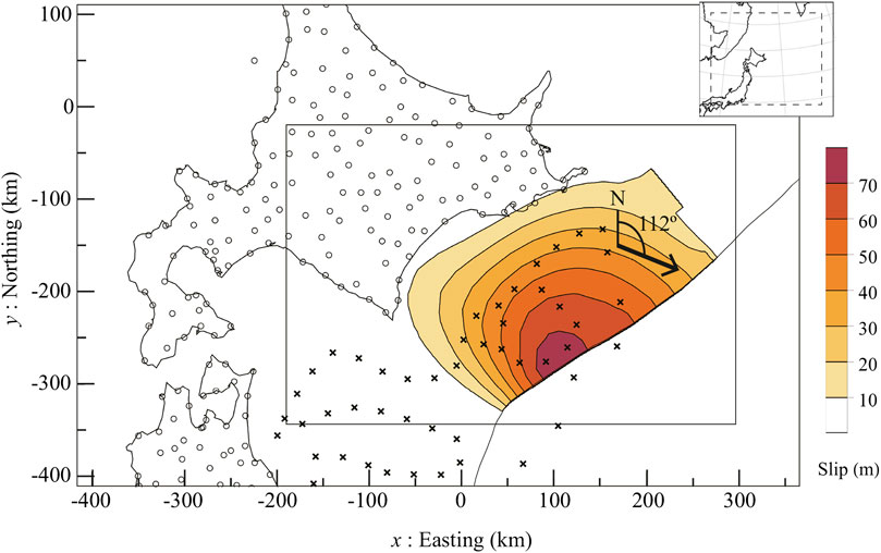
FIGURE 1. Reference spatial distribution of coseismic fault slip is shown as color contour. The direction of the slip was uniform in the 112° clockwise from north direction. The rectangle (solid line) is the target area for estimating the fault slip distribution. The curved thin solid line indicates the trench axis. The GNSS observation points are represented by circles, and the S-net and PG observation points are represented by crosses. The target range of the finite element model is indicated with dotted lines in the inset figure.

Much like with the Japan Trench, the Kuril Trench is an area where the Pacific plate subducts. Based on the distribution of tsunami deposits, it has been proposed that both segments off of Tokachi and Nemuro ruptured in the Seventeenth century (Nanayama et al., 2003). It has also been noted that the slip characteristics of this earthquake were similar to those of the 2011 Tohoku-Oki earthquake, which may have led to an 9M-class earthquake with a large slip in the shallow part of the plate interface (Ioki and Tanioka, 2016). In fact, traces of 15 tsunami deposits that span the past 6,000 years have been found (Sawai, 2020), and given the interval between the event of the Seventeenth century and the preceding event (some point in the 12th or 13th century), and the interval since the previous event, the indications are that a similar largest-class tsunami is imminent (Cabinet Office, 2020b). Furthermore, from the crustal deformation data on the land area, it is estimated that the slip-deficit that corresponds with the past source area is expanding (Hashimoto et al., 2012), and a seismic gap off the coast of Nemuro with low microseismic activity was noted by Takahashi and Kasahara (2013). It is possible that the plate interface at this region, including the shallow part of the plate interface, is strongly locked and has accumulated some slip-deficit. As part of an observation network in the area, submarine cable pressure sensors have been operational at two points off Kushiro for a long period, while the S-net system installed after the 2011 Tohoku-Oki earthquake covers the entire source area. Furthermore, to directly measure the seafloor deformation in the interseismic period, Tohoku University and Hokkaido University have jointly established a seafloor geodetic observation network with the aim of measuring the current interplate locking at the Kuril Trench off Nemuro. Specifically, three GNSS-A observation points and one seafloor acoustic ranging observation point were installed during the joint cruise KS-19‐12 of the Tohoku Marine Ecosystem Research Vessel ‘Shinseimaru’, conducted in July 2019. As such, the Kuril Trench was considered to be the most suitable area for conducting the current research.

We use the geometry of the plate interface used in the tsunami hazard scenario from the Cabinet Office (Disaster Management) as announced in 2019 (Yokota et al., 2017) and the coseismic slip distribution data (Cabinet Office, 2020a, page 4), respectively, which are both based on an array of scientific knowledge. However, as the Cabinet Office’s disaster management scenario assumes the occurrence of the largest possible tsunami, the slip distributes not only in the target area off Tokachi and Nemuro but also in the eastward area, where no real-time onshore nor off shore observation stations. Thus, to exclude the area outside of the observation network from the target analysis area, we use the slip distribution contained in the digital data provided by the Cabinet Office but with the eastern part removed for the reference slip distribution (see Figure 1). In terms of the plate interface geometry and topography, the digital elevation model data provided by the Cabinet Office is used. To appropriately handle the effects of the topography and plate interface geometry, a detailed finite element (FE) model is constructed, and the crustal deformation is calculated with high accuracy, as described in the next section. The reference interseismic slip-deficit distribution per year (Figure 2) was adjusted such that the maximum value will be 8 cm, as the relative velocity between the plates in this region is around 8 cm/year (Itoh et al., 2019), in the opposite direction at the time of the earthquake as back-slip method in Savage (1983) (i.e., the direction in which the slip-deficit occurs).

FIGURE 2

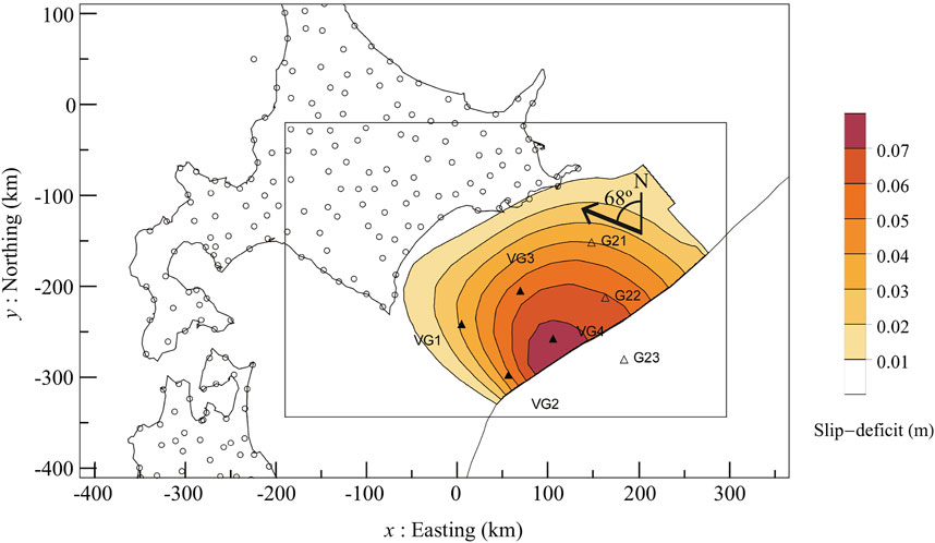
FIGURE 2. Reference spatial distribution of interseismic slip-deficit in one year is shown as color contour. The direction of the slip-deficit was uniform in the 68° counter-clockwise from north direction. The curved thin solid line indicates the trench axis. The position of GNSS observation points, GNSS-A observation points (G21, G22, G23), and the virtual GNSS-A observation points (VG1–VG4) are represented by circles, empty triangles, and filled triangles, respectively.

Since the purpose of this study is to quantitatively investigate the effect of observation error on the estimation of slip distribution, it was necessary to calculate the crustal deformation for the aforementioned reference slip distribution at each observation point, and then to provide a prescribed pseudo error for the observation data. In terms of observation data, we assume the measurement of crustal deformation via onshore GNSS, the measurement of vertical crustal deformation via OBP sensors (S-net, PG1, PG2), and the measurement of horizontal and vertical crustal deformation via GNSS-A. The measurement precision when using crustal deformation observation in terms of both land and seafloor for coseismic (precision available in real-time) and interseismic (precision obtained by post analysis) periods are shown in Table 1. Here, the covariance is assumed to be zero. Detailed information on the estimation of error for each observation sensor is included in Appendix section

TABLE 1

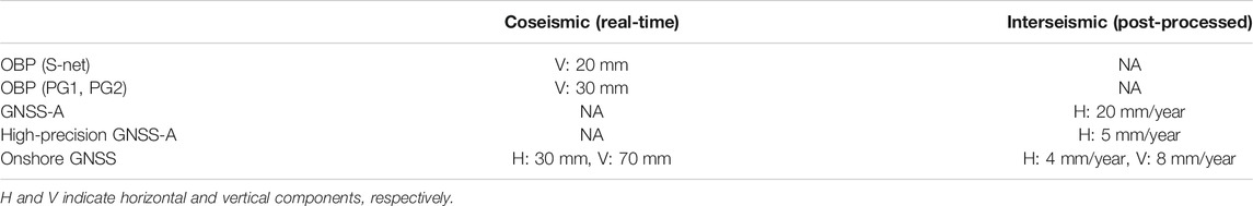
TABLE 1. Precision of the detection level of the crustal deformation for each sensor in coseismic and interseismic time.

2 Methodology

2.1 Computation of Green’s Functions Considering Three-Dimensional Crust Structure

We can expect improvement to the accuracy of fault slip distribution estimation when using Green’s functions that reflect the three-dimensional (3D) crust structure with the surface topography (e.g., Williams and Wallace, 2018). Here, we used the finite-element method (FEM) with unstructured elements to compute Green’s functions for the crustal deformation due to fault slip, since this method is suitable for solving problems with complex geometries and analytically satisfies the traction-free boundary condition at the surface (Ichimura et al., 2016). The fault slip could be evaluated using the split-node technique devised by Melosh and Raefsky (1981) and a clamped boundary condition was applied at the sides and bottom of the FE model. In general, it is difficult to generate large-scale 3D FE models that reflect the complex crust structure with high fidelity. Here, we generated such a model that was comprised of second-order tetrahedral elements using the automatic and robust meshing method devised by Ichimura et al. (2016). As the computational cost of FE analyses with large-scale models can be potentially huge, which was the case with this paper, FE solvers that can reduce the computation costs were proposed (Ichimura et al., 2016). The FE solver developed in Ichimura et al. (2016) enabled fast analysis on CPU-based systems. For conducting further large-scale analysis, we ported this FE solver to GPUs using OpenACC, which is a programming model with high portability.

2.2 Inversion Analysis Based on Green’s Functions

We estimated the fault slip distribution using geodetic data observed at N points on the surface using Green’s functions computed via the FE analysis method. We can represent the spatial distribution of fault slip $\mathit{s}\left(\mathit{x}\right)$ using a linear combination of M basis functions ${\mathit{X}}_m\left(\mathit{x}\right)$

$\mathit{s}\left(\mathit{x}\right)={\displaystyle \sum _{m=1}^m{a}_m{X}_m\left(\mathit{x}\right)},(1)$

where $\mathit{a}$ is the set of model parameters. The crustal deformation during fault slip is considered to be linear elastic. We can describe the equation representing the displacement response at the observation points on the ground surface ${\mathit{g}}_m$ for a unit fault slip ${\mathit{X}}_m$ as

$\mathit{d}=\mathit{Ga}+\mathit{e},(2)$

where $\mathit{d}$ is the vector of the surface displacements at the observation points, $\mathit{G}$ is the observation matrix that is comprised of the $g_i$ components of Green’s functions, and $\mathit{e}$ is the normally distributed errors with mean 0 and covariance matrix $\mathbf{\sum }$. When computing slip distribution in high resolution, the inverse problem may become indeterminate (the number of model parameters M may become larger than the number of observation channels N), and even if $M<N$, the system may become unstable and the solution may become highly sensitive in terms of noise. For the stabilization of these issues, it is essential to regularize the solution using prior information of the slip distribution. One approach to this involves minimizing an objective function such as

$\Phi \left(\mathit{a}\right)={\left(\mathit{d}-\mathit{Ga}\right)}^T{\mathbf{\sum }}^{-1}\left(\mathit{d}-\mathit{Ga}\right)+\lambda r(3)$

with,

$r={\displaystyle \int {\nabla }^{2}s\left(x\right)}\text{d}x,(4)$

where r is a roughness parameter used to penalize slip distribution with unrealistic oscillation in high frequencies. When using discretization based on finite difference approximations, the roughness can be represented as $r={\mathit{a}}^T\mathit{La}$, with a positive-semidefinite matrix $\mathit{L}$. The slip distribution of fault slip $\mathit{s}$ can be determined such that the objective function is minimized, given a specific value for λ. One common method used to determine λ is the k-fold cross validation method. Here, the observation dataset was split into k subsets, and the model parameters $\mathit{a}$ were estimated using the data in the $k-1$ subsets, with the remaining subset used to compute the validation error. The λ with the smallest total validation error is used in the final solution.

3 Numerical Experiments

We estimated the coseismic slip distribution and the interseismic slip-deficit distribution off Tokachi and Nemuro using the proposed inversion method. To verify the effect of the precision of the observation data and the presence of various observation points on the estimation accuracy, a reference solution must be generated for comparison with the estimated solutions. We obtained artificial observation data by applying the FE analysis to the reference slip distribution and adding the assumed noise to it. Using these artificial observation data, we estimated the slip distribution at the fault plane via the developed inversion method. To evaluate the difference in estimation accuracy with/without observation points and with varying observation precision, we introduced a Monte Carlo approach involving the inversion for 4,000 artificial observation datasets with different noise patterns for each case. From each inversion result, we verified the error distribution and the uncertainty in the estimated seismic slip and slip-deficit.

For the crustal structure data, we used the surface topography and the plate boundary set by the Cabinet Office’s disaster prevention division (Yokota et al., 2017), as described in Section 1.2. The crustal structure data were projected onto the 13th system of the Japanese plane orthogonal coordinate system, with the target domain set between coordinates of −1,053 km ≤ x ≤ 1,332 km in the east-west direction, −1,048 km ≤ y ≤ 922 km in the north-south direction, and −1,500 km ≤ z ≤ 0 km in the vertical direction. Since the Cabinet Office disaster prevention model assumes a homogeneous medium, the crustal structure was modeled as two layers with the same physical properties (rigidity is 40 GPa and Poisson’s ratio is 0.25), with the plate boundary in between. Figure 3 shows the FE model generated by discretizing the target model with minimum element size $ds$ = 1,620 m. The FE model consisted of 12,118,109 second-ordered tetrahedral elements with 50,050,911 degrees of freedom.

FIGURE 3

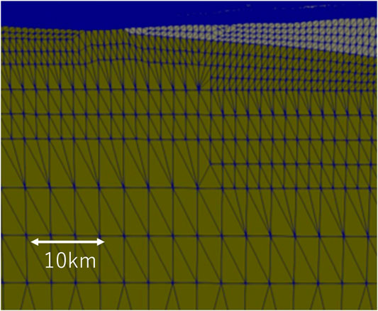
FIGURE 3. Overview and close-up view of the FE model.

The area of the fault plane for which Green’s functions were calculated was −189 km ≤ x ≤ 297 km and −344 km ≤ y ≤ 20 km. As a basis function of the fault slip distribution, we introduced a unit fault slip, which was designated as a bicubic B-spline curve of the grid. The grid points were set 32.4 km apart inside the target area, and the points outside the fault plane were excluded. Since the number of fitting points was 117 and the slip distribution in the x and y directions on the fault plane was considered, $2\times 117=234$ Green’s functions were calculated. The roughness used as regularization was provided via finite difference method using values on grid points. At this time, a virtual grid point with zero values was placed on the outer circumference of the area and regularization was applied to the range that included these points. To calculate the 234 Green’s functions, two IBM Power System AC922 compute nodes with dual 16-core IBM POWER9 2.60 GHz CPUs and 4 NVIDIA Tesla V100 GPUs were used. Thus, in total, eight GPUs were used in parallel with eight MPI processes. While the computation of the 234 Green’s functions via 50 million degrees of freedom 3D FE models would generally require huge computational costs, the analysis time was significantly reduced through using a suitable analysis algorithm with GPU implementation, which allowed for computing each Green’s function in less than 10 s.

In the following subsections, we estimate the coseismic slip and the interseimic slip-deficit distributions using the observation points shown in Figures 1, 2 and discuss the obtained analysis results.

3.1 Results and Discussion for Coseismic Slip

We conducted estimations using two sets of observation data: 1) land GNSS, and 2) land GNSS and OBP. For the fault slip estimation immediately after the occurrence of an earthquake (within around 5 min), only GNSS results is used. Compared with the reference solution (Figure 1), the overall picture, including larger slip (>60 m) near the trench axis, is captured only by the land data (Figure 4A left). However, the residual near the trench axis was locally 10 m or more (several tens of percent or more) at $x\sim 100$ km (Figure 4A, middle). Here is near the peak of the reference slip and results in an underestimation, while the east side where the slip decreases ($x>250$ km) results in an overestimation. The result demonstrated that it is difficult to accurately attain the heterogeneous slip distribution near the trench axis using land-based GNSS data alone, and that the estimation accuracy of the initial wave source of the resulting tsunami is low in this region. On the other hand, when we include the OBP data, the estimation accuracy of the slip distribution near the trench axis becomes much higher (Figure 4B). Hence, if the OBP data are inputted into the REGARD system, this is expected to improve the accuracy of estimating the tsunami height and its inundation distribution, which is of great social importance. When using the OBP data of an earthquake to measure the crustal deformation, noise such as the dynamic water pressure fluctuations associated with the seismic waves and the fluctuations associated with the tsunami will be included in the measurement data. To estimate the crustal deformation accurately in a short period of time, it is important to appropriately remove such noise. By using the proposed method, it is possible to quantify the effects of these forms of noise.

FIGURE 4

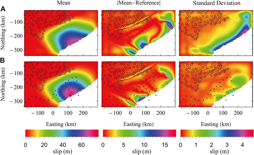
FIGURE 4. Mean, absolute error between mean and reference solution, and standard deviation of coseismic fault slip distribution with 4,000× Monte Carlo inversions using (A) GNSS data and (B) GNSS and OBP data. The average standard deviation is (A) 0.847 m and (B) 0.439 m, respectively. The position of GNSS and OBP stations are represented by circles and cosses, respectively.

The above results are the cases where model errors are ignored. If model errors are taken into account, we can imagine that the recovery to the reference model will be worse in any case. However, the important question here is how the effect of addition of offshore observation points changes when model errors are considered. Based on the results in a previous study (Yamaguchi et al., 2017a), the standard deviation in slip estimation at the area away from the observation points is twice or more comparing with that below the observation point when P and S wave velocity varies in 10 and 20% and density varies in 15% for the 3D heterogeneous structure. This means that the advantage of addition of observation points in the offshore area is expected to be more pronounced with model error than illustrated in Figure 4. Additionally, the analyses with model error requires plenty number of calculations for Green’s functions of various 3D heterogeneous structures with model error but we think it is possible to demonstrate with GPU application as in this study and also Yamaguchi et al. (2017a), Yamaguchi et al. (2017b).

3.2 Results and Discussion for Interseismic Slip-Deficit

The cable OBP data, which is useful for measuring coseismic seafloor deformation as shown in Section 3.1, is not used in interseismic slip estimations since it is difficult to correct any sensor specific drifts. Here, GNSS-A plays an important role. As noted in Appendix, the GNSS-A observation error can be significantly reduced by increasing the frequency of observations (Yokota et al., 2016). Here we conducted four cases using different types of observation data: 1) land GNSS, 2) land GNSS and GNSS-A, 3) land GNSS and high-precision GNSS-A, and 4) land GNSS and high-precision GNSS-A with additional GNSS-A points that are not presently installed in the target area. The result of the land GNSS only shows that larger slip-deficit toward the trench axis cannot be recovered with considerable underestimation (Figure 5A). The result differs significantly from the coseismic slip case only with the land data in Section 3.1, even though the relative distribution is the same. This is probably because the signal-to-noise ratio is an order of magnitude smaller in the case of slip-deficit in one year than in the case of large slip caused by the 9M earthquake, and it is not possible to constrain the larger slip-deficit away from the observation points as indicated clearly in Figure 5A. Currently, GNSS-A observations along the Kuril Trench are conducted around once a year by Tohoku University and other institutions (Honsho et al., 2019). The error of the displacement velocity obtained is expected to be around 20 mm/year, which is large compared to the cases using GNSS-A observations with higher frequency. The estimation results for the land GNSS and GNSS-A in offshore area are shown in Figure 5B. Even when using such seafloor observations with the relatively large error, it is clear that the slip-deficit rate is recovered better near the trench axis than when using land observations alone. Furthermore, if high frequency observations (more than several times a year, as in regions such as southwest Japan) could be realized, the error in the magnitude of the slip-deficit rate would be quantitatively suppressed to several tens of percent or less (Figure 5C). In particular, the error is less than 10% just below the GNSS-A observation point. On the other hand, the part of $x=0-100$ km, where there is no observation point and the peak of the slip-deficit is located, is still underestimated. While it is difficult to carry out observations with high frequency using ships, the development of automatically repeated observations using wave gliders (Iinuma et al., 2012, submitted to this issue) are in progress, which means we can expect the realization of such high accuracy estimations in the near future. Finally, the results of the slip estimation when adding four virtual GNSS-A observation points in the segments off Tokachi are shown in Figure 5D. The estimation accuracy of the heterogeneity of the plate coupling in the strike direction of the plate subduction is clearly improved by adding the observation points just above the peak slip-deficit area. The intervals of additional GNSS-A points are around 70 km (similar to the existing ones). As a result, there are observation points within a horizontal distance of about 50 km from each source of the slip-deficit, and the estimation error becomes less than 10% for the whole offshore area. When adding GNSS-A observation points in the future, it will be important to determine the installation position after performing such a quantitative accuracy evaluation for a more effective estimation of the slip-deficit distribution. For this purpose, we can apply the present method to various combinations of possible distributions of slip-deficit rates and additional observation points of feasible number with a brute-force search or with a non-linear optimization method (e.g., Sathiakumar et al., 2017).

FIGURE 5

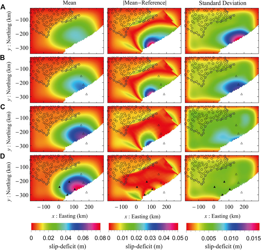
FIGURE 5. Mean, absolute error between mean and reference solution, and standard deviation of interseismic fault slip-deficit distribution with 4,000× Monte Carlo inversions using (A) GNSS data, (B) GNSS and GNSS-A data, (C) GNSS and high-precision GNSS-A data, and (D) GNSS and high-precision GNSS-A data with additional GNSS-A observation points. The average standard deviation for each case was (A) 0.0040 m, (B) 0.0041 m, (C) 0.0046 m, and (D) 0.0034 m, respectively. The position of GNSS, GNSS-A, and the virtual GNSS-A stations are represented by circles, empty triangles, and filled triangles, respectively.

To examine the effect of the improvement in observation precision and the addition of observation points in more detail, a pointwise evaluation was performed at the installed GNSS-A observation point G22 and the virtual GNSS-A observation point VG1 (Figure 2 shows the position of the observation points and Figures 6, 7 show the results). In Figure 6, the solid vertical line represents the true response value for the reference fault slip, while the broken line represents the modeled probability distribution when considering the observation errors listed in Table 1. The histogram represents the predicted response values obtained by the inversion of the pseudo observation data with the aforementioned 4,000 patterns of noise. In the case of the current GNSS-A observation measurement method, the observation precision is 20 mm/year, which is comparable with the magnitude of the horizontal crustal deformation caused by the slip-deficit of 80 mm/year. Thus, the weight of the observed value is considered to be small and the regularization is deemed to have performed strongly during the optimization process. As such, the predicted distribution obtained from the estimated slip-deficit had a large deviation from the modeled distribution (Figure 6A, G22 and VG1). However, when the observation precision was improved to 5 mm/year, the spatial distribution that reproduces the observed displacement was obtained (Figure 5C), which resulted in obtaining an almost identical probability distribution among the predicted and modeled distributions (Figure 6B, G22). Note that the predicted distribution for the virtual GNSS-A site (VG1), which is not included in the inversion, still shows deviation from the modeled distribution (Figure 6C, VG1). Furthermore, by adding virtual GNSS-A observation points, the spatial distribution of the slip-deficit was reproduced more accurately and the standard deviation became smaller (Figure 5D). Thus, a probability distribution with a slightly smaller variance than the modeled probability distribution was obtained for both of the observation points (Figure 6C, G22 and VG1).

FIGURE 6

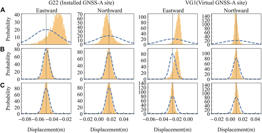
FIGURE 6. Horizontal displacement distribution at observation points G22 and VG1 (see Figure 2 for the position of the observation points). True predicted distribution (dotted line), true observed value (solid vertical line, as variance is zero), and predicted distribution obtained from the optimization results (histogram). (A) GNSS and GNSS-A (B) GNSS and high-precision GNSS-A, (C) GNSS and high-precision GNSS-A with additional GNSS-A observation points.

FIGURE 7

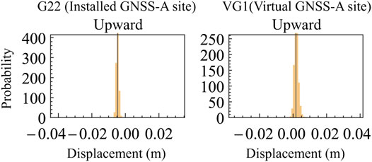
FIGURE 7. Vertical displacement distribution at observation points G22 and VG1 (see Figure 2) for the case of GNSS and high-precision GNSS-A and additional GNSS-A observation points. True observed value (solid vertical line, as variance is zero) and the predicted distribution obtained from the optimization results (histogram) are shown.

Conventionally, the measurement of the horizontal position was the main purpose of GNSS-A; however, in recent years, methods for realizing high-precision measurement in the vertical direction have been developed. Thus, it is meaningful to consider how much precision is required in the vertical displacement measurement to improve interseismic slip-deficit estimations. For a low-angle fault, the vertical displacement is smaller than the horizontal displacement, which means the difference and variance between the true value and the predicted value becomes smaller. Therefore, if the results of this study as shown in Figure 7 are accepted, the vertical displacement of GNSS-A is unlikely to contribute to the improvement in the accuracy of interseismic slip-deficit distribution estimations, unless a high observation precision within several millimeters is realized. However, based on the discussion about model error in Section 3.1, it is highly possible that the use of the correct Green’s function (without model error) has led to the good reproduction of vertical displacement using horizontal component observation constraints alone. If we introduce model error, horizontal component becomes not enough to constrain the slip distribution and the contribution of the vertical component becomes larger.

4 Conclusion

The purpose of this manuscript is to quantify the effectiveness of the offshore data for the slip estimation especially near the trench axis. Our results demonstrate the effectiveness of the observation of seafloor crustal deformation near the trench axis, as well as the advancement in the modeling, including in terms of topography and plate geometry. For the coseismic slip, the heterogeneous distribution near the trench axis can be reproduced when we include the cable OBP data, which cover whole the offshore source area. Furthermore, it was demonstrated that the interseismic slip-deficit distribution in the shallow part of the subducting plate interface can be reproduced with high accuracy by improving the precision of the seafloor crustal deformation observations (i.e., increasing the observation frequency of GNSS-A). It was also demonstrated that the estimated resolution of the slip-deficit in the strike direction in this area can be improved and the estimation error becomes less than 10% for the whole offshore area by adding four GNSS-A observation points off Tokachi to the currently installed off Nemuro with about 70 km interval. However, the cost of increasing the number of observation points will involve not only the installment costs but also the additional costs for conducting the measurements on each occasion. Thus, obtaining the maximum effect with the minimum number of additional observation points is crucial, and the proposed method applying various combinations of possible distributions of slip-deficit and additional observation points is expected to be useful for this purpose. Meanwhile, it was shown that higher observation precision than that for the horizontal components is required for the vertical components of the observations to become useful for the improvement of the estimation of slip-deficit distribution. However, it is highly possible that this finding was due to the use of exact Green’s functions, and it is thus necessary to conduct additional research by extending the proposed method for the consideration of model error and to conduct appropriately extended evaluations. In addition, a numerical experiment was conducted with assuming a slip-deficit distribution that would suit a preparation process for a large 9M-class earthquake. However, seismic events at a plate interface can occur on a smaller scale (e.g., Honsho et al., 2019). In recent years, seafloor acoustic observations that range over the trench axis at the shallowest plate interface have also been performed by various researchers (e.g., Yamamoto et al., in preparation). Here, an improvement to the structure model is an expected requirement for the accurate reproduction of smaller plate interface events and the reproduction of the phenomena on a scale of around 10 km or less that straddle the trench axis. It is expected that the understanding of the phenomena that occur at the plate interface will be further advanced by improving both the modeling and the observation. It should be noted that our analysis used the exact solution as the Green’s function, which meant the analysis was performed with a model error of zero. In the case of actual data analysis, such level of estimation accuracy cannot be expected since there is an error in the underground crustal structure model. However, it is expected that such analyses with model error will enable a quantitative examination of the improvement in the accuracy of the results through the improvement in observation precision and addition of observation points, even for actual data. Furthermore, we consider that the quantification procedure is applicable to other slip and slip-deficit distribution patterns and other subduction zones as well.

Data Availability Statement

The original contributions presented in the study are included in the article/Supplementary Material, further inquiries can be directed to the corresponding author.

Author Contributions

SM, TI, TH, and YO formulated the investigation. SM, TI, and KF developed the finite-element method, SM and TI developed the inversion method, and SM conducted the numerical experiments. TH and YO provided information and discussion related to the observation methods. All authors contributed to the article.

Funding

This work was supported by the Ministry of Education, Culture, Sports, Science and Technology of Japan (MEXT) as “Program for Promoting Researches on the Supercomputer Fugaku” (Large-scale numerical simulation of earthquake generation, wave propagation and soil amplification: hp200126) and by JSPS KAKENHI (JP18H05239).

Conflict of Interest

The authors declare that the research was conducted in the absence of any commercial or financial relationships that could be construed as a potential conflict of interest.

Acknowledgments

We thank the two anonymous reviewers for constructive comments. Digital data of surface topography, plate boundary and coseismic slip distribution are given by Cabinet Office, Disaster Management. This work was supported by the Ministry of Education, Culture, Sports, Science and Technology of Japan (MEXT) as “Program for Promoting Researches on the Supercomputer Fugaku” (Large-scale numerical simulation of earthquake generation, wave propagation and soil amplification: hp200126) and by JSPS KAKENHI (JP18H05239). This work was partly supported by MEXT, under its Earthquake and Volcano Hazards Observation and Research Program.

Appendix

Here, we explain the characteristics of each observation method and the estimation of observation precision used in this study.

Cable OBP

OBP systems present observation sensors that allow us to continuously measure vertical crustal displacements and tsunami heights through measuring the pressure of the water column with a water pressure gauge installed on the seafloor. In recent years, cable OBP observations have been deployed mainly for the purpose of the immediate prediction of tsunamis in Japan. The obtained OBP data contain not only the crustal deformation but also the other contributions, including those of the tidal component, the non-tidal component, and the sensor-specific drift component. However, it is particularly difficult to remove the sensor-specific drift component, which means it is currently difficult to capture the slow crustal deformation in the interseismic period using OBP data. This form of data was thus not used for the interseismic slip-deficit estimation in this study. Meanwhile, the observation of coseismic crustal deformation, postseismic crustal deformation, and unsteady crustal deformation, which are phenomena with shorter time scales, has been carried out by numerous researchers (e.g., Baba et al., 2006; Ito et al., 2011; Ohta et al., 2012a; Hino et al., 2014; Sato et al., 2017; Kubota et al., 2020). Here, Baba et al. (2006) estimated the postseismic slip distribution of the 2003 Tokachi-Oki earthquake using two OBP sensors (PG1, PG2) installed off the coast of Tokachi and onshore GNSS data, with the authors assuming that the standard deviation of the daily OBP data after correcting with the thermometer data was 2 hPa (around 2 cm in terms of crustal deformation). Meanwhile Kubota et al. (2020) used the OBP data obtained from the S-net laid in the Japan Trench and the southern part of the Kuril Trench to analyze the millimeter-scale micro tsunami to estimate the fault model of the Mw6.0 earthquake that occurred off Sanriku. Here, the short-term stability of the S-net OBP data before and after the earthquake was 1 hPa (around 1 cm in terms of crustal deformation). To understand the crustal deformation that occurs during an earthquake, it is necessary to calculate the difference before and after the earthquake. Therefore, the error before and after the earthquake was propagated to obtain the estimation error of the displacement during the earthquake. As a result, estimation errors of 30 mm for PG1 and PG2 off Tokachi and 20 mm for S-net were used in terms of the displacement that occurs during earthquakes obtained in real-time (Table 1). In reality, the accuracy is likely to be degraded due to the effects of tsunami, but for simplicity, we used this value here.

GNSS-A

GNSS-A presents a technology that estimates the relative position of the reference station installed on the seafloor according to the acoustic distance measurement from the sea surface platform, with the position of the sea surface platform obtained via GNSS. The seafloor crustal deformation is then measured by combining these results. Here, we considered the precision of estimating the displacement in the interseismic period via GNSS-A. Honsho et al. (2019) estimated the postseismic crustal deformation of the 2011 Tohoku-Oki earthquake in detail from the data of 20 GNSS-A stations installed in the Japan Trench. Here, the estimation precision of the displacement velocities at 20 points based on the data covering a four-year period was found to be around 13 mm/year for both the east-west and the north-south components. Therefore, in this study, the current observation error was rounded up to 20 mm/year. In addition, Yokota et al. (2016) observed the GNSS-A seafloor observation network that is installed in the Nankai Trough more than several times a year, and estimated the horizontal velocity with high precision (around 4 mm/year). The estimation error of these displacement velocities depended on the observation frequency and the precision of individual campaign observations. From these results, we assumed 5 mm/year for the errors of high-precision interseismic horizontal velocity observation via frequent GNSS-A measurements.

Onshore GNSS

In recent years, many attempts have been made to immediately estimate the magnitude of a large earthquake using real-time GNSS data (e.g., Ohta et al., 2012a; Kawamoto et al., 2016; Kawamoto et al., 2017). Here, Ohta et al. (2012a) demonstrated that the crustal deformation can be grasped relatively accurately even in real-time using RTK-GNSS data. Here, the authors clarified that the accuracy of the RTK-GNSS positioning depended upon the baseline length, and that the horizontal and vertical precision was around 20 and 50 mm, respectively, at the 500 km baseline. Similarly, Kawamoto et al. (2017) calculated the daily coordinate value stability at 146 points of the GEONET system, and obtained a standard deviation value of 10–15 mm for the horizontal component and 42 mm for the vertical component. Since the difference of the data before and after the earthquake was used to estimate the amount of permanent displacement due to the earthquake, the horizontal and vertical precision of the coseismic displacements in real time were assumed to be 30 and 70 mm, respectively.

Next, we considered the precision of interseismic displacement measurement using land-based GNSS. Itoh et al. (2019) discussed the crustal deformation following the 2003 Tokachi-Oki earthquake using onshore GNSS and OBP data. Here, the authors removed the step-like fluctuations due to yearly peripheral components and equipment replacement from the daily GEONET coordinate values, obtained the monthly coordinate values by down sampling them, and evaluated the quartile deviation of the coordinate values within the month. As a result, the horizontal and vertical measurement error was found to be 2 and 8 mm, respectively. Elsewhere, Suito (2016) evaluated GEONET’s fault slip detection capability. Here, the author estimated the average trend and the annual and semiannual components from the coordinate time series for each year from January 1, 2006 to December 31, 2010 and from January 1, 2010 to December 31, 2010. Computing the residual by subtracting the average trend, annual, and semiannual components from the observation data, average $1\sigma$ of the residual was computed for the two periods. As a result, the horizontal and vertical average deviation of all GEONET points were found to be 3.34 and 7.35 mm, respectively. Based on these results, the precision of land-based GNSS data was assumed to be 4 mm/year for the horizontal component and 8 mm/year for the vertical component.

References

Agata, R., Hori, T., Ariyoshi, K., and Ichimura, T. (2019). Detectability analysis of interplate fault slips in the nankai subduction thrust using seafloor observation instruments. Mar. Geophys. Res. 40, 453. doi:10.1007/s11001-019-09380-y

CrossRef Full Text | Google Scholar

Baba, T., Hirata, K., Hori, T., and Sakaguchi, H. (2006). Offshore geodetic data conducive to the estimation of the afterslip distribution following the 2003 Tokachi-oki earthquake. Earth Planet. Sci. Lett. 241, 281–292. doi:10.1016/j.epsl.2005.10.019

CrossRef Full Text | Google Scholar

Cabinet Office, D. M. (2020a). Figures and tables for megathrust earthquake models along the Japan Trench and the Kuril Trench. Tokyo: Cabinet Office.

Cabinet Office, D. M. (2020b). Report for megathrust earthquake models along the Japan Trench and the Kuril Trench. Tokyo: Cabinet Office.

Gagnon, K., Chadwell, C. D., and Norabuena, E. (2005). Measuring the onset of locking in the Peru-Chile trench with GPS and acoustic measurements. Nature 434, 205–208. doi:10.1038/nature03412

PubMed Abstract | CrossRef Full Text | Google Scholar

Hashimoto, C., Noda, A., and Matsuura, M. (2012). The Mw 9.0 northeast Japan earthquake: total rupture of a basement asperity 189. Geophys. J. Int. 1–5. doi:10.1111/j.1365-246X.2011.05368.x

CrossRef Full Text | Google Scholar

Hino, R., Inazu, D., Ohta, Y., Ito, Y., Suzuki, S., Iinuma, T., et al. (2014). Was the 2011 Tohoku-Oki earthquake preceded by aseismic preslip? Examination of seafloor vertical deformation data near the epicenter. Mar. Geophys. Res. 35, 181–190. doi:10.1007/s11001-013-9208-2

CrossRef Full Text | Google Scholar

Honsho, C., Kido, M., Tomita, F., and Uchida, N. (2019). Offshore postseismic deformation of the 2011 Tohoku earthquake revisited: application of an improved GPS‐acoustic positioning method considering horizontal gradient of sound speed structure. J. Geophys. Res. Solid Earth 124, 5990–6009. doi:10.1029/2018JB017135

CrossRef Full Text | Google Scholar

Ichimura, T., Agata, R., Hori, T., Hirahara, K., Hashimoto, C., et al. (2016). An elastic/viscoelastic finite element analysis method for crustal deformation using a 3-D island-scale high-fidelity model. Geophys. J. Int. 206, 114–129. doi:10.1093/gji/ggw123

CrossRef Full Text | Google Scholar

Ichimura, T., Agata, R., Hori, T., Satake, K., Ando, K., Baba, T., et al. (2017). Tsunami analysis method with high-fidelity crustal structure and geometry model. J. Earthquake Tsunami 11, 1750018. doi:10.1142/S179343111750018X

CrossRef Full Text | Google Scholar

Iinuma, T., Hino, R., Kido, M., Inazu, D., Osada, Y., Ito, Y., et al. (2012). Coseismic slip distribution of the 2011 off the Pacific Coast of Tohoku Earthquake (M9.0) refined by means of seafloor geodetic data. J. Geophys. Res. 117, 18–91. doi:10.1029/2012JB009186

CrossRef Full Text | Google Scholar

Imano, M., Kido, M., Honsho, C., Ohta, Y., Takahashi, N., and Fukuda, T. (2019). Assessment of directional accuracy of GNSS-Acoustic measurement using a slackly moored buoy. Prog. Earth Planet. Sci. 6, 1–14. doi:10.1186/s40645-019-0302-1

CrossRef Full Text | Google Scholar

Ioki, K., and Tanioka, Y. (2016). Re-estimated fault model of the 17th century great earthquake off Hokkaido using tsunami deposit data. Earth Planet. Sci. Lett. 433, 133–138. doi:10.1016/j.epsl.2015.10.009

CrossRef Full Text | Google Scholar

Ito, Y., Tsuji, T., Osada, Y., Kido, M., Inazu, D., Hayashi, Y., et al. (2011). Frontal wedge deformation near the source region of the 2011 Tohoku-Oki earthquake. Geophys. Res. Lett. 38, 35–83. doi:10.1029/2011GL048355

CrossRef Full Text | Google Scholar

Itoh, Y., Nishimura, T., Ariyoshi, K., and Matsumoto, H. (2019). Interplate slip following the 2003 tokachi‐oki earthquake from ocean bottom pressure gauge and land GNSS data. J. Geophys. Res. Solid Earth 124, 4205–4230. doi:10.1029/2018JB016328

CrossRef Full Text | Google Scholar

Kawamoto, S., Hiyama, Y., Ohta, Y., and Nishimura, T. (2016). First result from the GEONET real-time analysis system (REGARD): the case of the 2016 kumamoto earthquakes. Earth Planets Space 68. doi:10.1186/s40623-016-0564-4

CrossRef Full Text | Google Scholar

Kawamoto, S., Ohta, Y., Hiyama, Y., Todoriki, M., Nishimura, T., Furuya, T., et al. (2017). REGARD: a new GNSS-based real-time finite fault modeling system for GEONET. J. Geophys. Res. Solid Earth 122, 1324–1349. doi:10.1002/2016JB013485

CrossRef Full Text | Google Scholar

Kimura, H., Tadokoro, K., and Ito, T. (2019). Interplate coupling distribution along the Nankai Trough in southwest Japan estimated from the block motion model based on onshore GNSS and seafloor GNSS/A observations. J. Geophys. Res. Solid Earth 124, 6140–6164. doi:10.1029/2018JB016159

CrossRef Full Text | Google Scholar

Kinugasa, N., Tadokoro, K., Kato, T., and Terada, Y. (2020). Estimation of temporal and spatial variation of sound speed in ocean from GNSS-A measurements for observation using moored buoy. Prog. Earth Planet. Sci. 7, 1–14. doi:10.1186/s40645-020-00331-5

CrossRef Full Text | Google Scholar

Kubota, T., Saito, T., and Suzuki, W. (2020). Millimeter‐scale tsunami detected by a wide and dense observation array in the deep ocean: fault modeling of an Mw 6.0 interplate earthquake off Sanriku, NE Japan. Geophys. Res. Lett. 47, 1–11. doi:10.1029/2019GL085842

CrossRef Full Text | Google Scholar

Melosh, H. J., and Raefsky, A. (1981). A simple and efficient method for introducing faults into finite element computations. Bull. Seismol. Soc. Am. 71, 1391–1400.

Google Scholar

Mochizuki, M., Uehira, K., Kanazawa, T., Kunugi, T., Shiomi, K., Aoi, S., et al. (2018). “S-net project: performance of a large-scale seafloor observation network for preventing and reducing seismic and tsunami disasters,” in OCEANS - MTS/IEEE Kobe Techno-Oceans (OTO), Kobe, Japan, May 29–31 (IEEE),1–4. doi:10.1109/OCEANSKOBE.2018.8558823

CrossRef Full Text | Google Scholar

Nanayama, F., Satake, K., Furukawa, R., Shimokawa, K., Atwater, B. F., Shigeno, K., et al. (2003). Unusually large earthquakes inferred from tsunami deposits along the Kuril trench. Nature 424, 660–663doi:10.1038/nature01864

PubMed Abstract | CrossRef Full Text | Google Scholar

Ohta, Y., Hino, R., Inazu, D., Ohzono, M., Ito, Y., Mishina, M., et al. (2012a). Geodetic constraints on afterslip characteristics following the March 9, 2011, Sanriku-oki earthquake, Japan, Geophys. Res. Lett. 39, 430. doi:10.1029/2012GL052430

CrossRef Full Text | Google Scholar

Ohta, Y., Kobayashi, T., Tsushima, H., Miura, S., Hino, R., Takasu, T., et al. (2012b). Quasi real-time fault model estimation for near-field tsunami forecasting based on RTK-GPS analysis: application to the 2011 Tohoku-Oki earthquake (Mw9.0). J. Geophys. Res. 117, 750. doi:10.1029/2011JB008750

CrossRef Full Text | Google Scholar

Ohta, Y., Inoue, T., Koshimura, S., Kawamoto, S., and Hino, R. (2018). Role of real-time GNSS in near-field tsunami forecasting. J. Disaster Res. 13, 453–459. doi:10.20965/jdr.2018.p0453

CrossRef Full Text | Google Scholar

Ohta, Y., Kobayashi, T., Hino, R., Demachi, T., and Miura, S. (2015). “Rapid coseismic fault determination of consecutive large interplate earthquakes: the 2011 Tohoku-Oki sequence”, in International Association of Geodesy Symposia, 143 (New York: Springer), 467–475. doi:10.1007/1345˙2015˙109

CrossRef Full Text | Google Scholar

Sato, T., Hasegawa, S., Kono, A., Shiobara, H., Yagi, T., Yamada, T., et al. (2017). Detection of vertical motion during a slow-slip event off the Boso Peninsula, Japan, by ocean bottom pressure gauges. Geophys. Res. Lett. 44, 2710–2715. doi:10.1002/2017GL072838

CrossRef Full Text | Google Scholar

Savage, J. C. (1983). A dislocation model of strain accumulation and release at a subduction zone. J. Geophys. Res. 88, 4984–4996. doi:10.1029/jb088ib06p04984

CrossRef Full Text | Google Scholar

Sawai, Y. (2020). Subduction zone paleoseismology along the Pacific coast of northeast Japan - progress and remaining problems. Earth-Science Rev. 208, 103261. doi:10.1016/j.earscirev.2020.103261

CrossRef Full Text | Google Scholar

Sathiakumar, S., Barbot, S. D., and Agram, P. (2017). Extending resolution of fault slip with geodetic networks through optimal network design. J. Geophys. Res. Solid Earth 122, 538–610. doi:10.1002/2017JB014326

CrossRef Full Text | Google Scholar

Suito, H. (2016). Detectability of interplate fault slip around Japan, based on GEONET daily solution F3. J. Geodetic Soc. Jap. 62, 109–120. 10.10072Fs11001-019-09380-y

Google Scholar

Takahashi, H., and Kasahara, M. (2013). “Spatial relationship between interseismic seismicity, coseismic asperities and aftershock activity in the southwestern kuril islands,” in Volcanism and subduction: the Kamchatka region, geophysical monograph series 172. Editors J. Eichelberger, E. Gordeev, P. Izbekov, M. Kasahara, and J. Lees (American Geophysical Union), 153–164.

Google Scholar

Williams, C. A., and Wallace, L. M. (2018). The impact of realistic elastic properties on inversions of shallow subduction interface slow slip events using seafloor geodetic data. Geophys. Res. Lett. 45, 7462–7470. doi:10.1029/2018GL078042

CrossRef Full Text | Google Scholar

Yamaguchi, T., Fujita, K., Ichimura, T., Hori, T., Hori, M., and Wijerathne, L. (2017a). Fast finite element analysis method using multiple GPUs for crustal deformation and its application to stochastic inversion analysis with geometry uncertainty. Proced. Comp. Sci. 108, 765–775. doi:10.1016/j.procs.2017.05.223

CrossRef Full Text | Google Scholar

Yamaguchi, T., Ichimura, T., Yagi, Y., Agata, R., Hori, T., and Hori, M. (2017b). Fast crustal deformation computing method for multiple computations accelerated by a graphics processing unit cluster. Geophys. J. Int. 210, 787–800. doi:10.1093/gji/ggx203

CrossRef Full Text | Google Scholar

Yokota, T., Nemoto, M., Matsusue, K., Takase, S., Takata, K., and Ikeda, M. (2017). Study on the plate model of the Pacific plate. JpGU-AGU Jt. Meet. SSS13–P04

Google Scholar

Yokota, Y., Ishikawa, T., Watanabe, S. I., Tashiro, T., and Asada, A. (2016). Seafloor geodetic constraints on interplate coupling of the Nankai Trough megathrust zone. Nature 534, 374–377. doi:10.1038/nature17632

PubMed Abstract | CrossRef Full Text | Google Scholar