A Refined Method to Analyze Insoluble Particulate Matter in Ice Cores, and Its Application to Diatom Sampling in the Antarctic Peninsula

Introduction

Ice cores are faithful recorders of changing climate over thousands of years (Alley, 2014). The chemical composition of ice reflects changes in atmospheric composition and circulation, while patterns in the seasonal deposition of chemical species allow accurate dating of ice cores at annual and sub-annual resolution (Legrand and Mayewski, 1997; Alley, 2010). Ice core chronologies are constructed from a variety of parameters, including absolute time markers and seasonal indicators (Wolff et al., 2010). Absolute time markers can be produced by large-magnitude volcanic eruptions. Their SO₂ emissions (Sigl et al., 2015) and tephra deposits (Davies et al., 2012) have provided numerous reference horizons in ice cores. Seasonal indicators include changes in the stable isotope composition of the ice, changes in the concentration of impurities and changes in the physical properties of ice, among others (Legrand and Mayewski, 1997). All these parameters are useful for establishing an ice core chronology, improving the dating accuracy when considered together.

The study of insoluble particles in ice has provided valuable information for reconstructing past climate. Among the insoluble particulate matter (IPM) present in ice, the insoluble particle fraction of dust (fine particles of solid matter) is the most abundant; hereafter, we refer to this component as ‘dust’. Dust flux, provenance and grain-size variability have been widely studied in ice cores (Delmonte et al., 2019). Their study has contributed significantly to the understanding of changes in atmospheric and terrestrial conditions over the last eight glacial cycles (Lambert et al., 2008). Additional and distinctive information about past environmental conditions can be extracted from the study of dust sub-sets, hereafter referred to as low concentration insoluble particulate matter (LC-IPM). This group includes pollen, cryptotephra, diatoms and black carbon, among others. Pollen in alpine ice cores has shown to present seasonal variations, helping to improve the accuracy of ice chronologies (Nakazawa and Fujita, 2006; Festi et al., 2015); pollen has also been studied in Greenland and other Arctic ice cores (Bourgeois et al., 2000; Brugger et al., 2019). The study of cryptotephra layers in ice cores provides valuable tie-points to link oceanic, terrestrial and atmospheric records (Dunbar et al., 2017; Cook et al., 2018). Diatoms in ice cores have the potential to reconstruct past atmospheric circulation (Allen et al., 2020). Black carbon studies in ice cores allowed tracking past variations in snow albedo and their climate forcing (McConnell et al., 2007; Osmont et al., 2018). Altogether, the study of LC-IPM in ice cores provides a valuable contribution to the study of past climate.

Several methods have been developed to study the total dust content and the particle-size distribution in ice samples (Ruth et al., 2003). These methods have been widely tested, validated and implemented, proving to provide accurate high-resolution records (Vallelonga and Svensson, 2014). However, dust measurement techniques do not differentiate the origin of each particle in the sample, for example, marine vs. terrestrial origin or local vs. long-range sources. Thus, they ignore the abundance, diversity and size distribution of the LC-IPM. Additionally, traditional methods to study dust do not analyze morphological or textural features in particles, omitting valuable information such as the formation of dust aggregates (Tison et al., 2015; Baccolo et al., 2018), microfossil preservation (Warnock and Scherer, 2015) or vesicles and shard shapes in cryptotephra (Dunbar and Kurbatov, 2011; Dunbar et al., 2017).

Previous studies have proposed various methods to study different LC-IPM in ice core samples. The ideal method should continuously extract LC-IPM with minimum losses and analyze the samples following an optimized approach to obtain statistically representative results. Several methods have been proposed to extract LC-IPM from discrete ice samples (Brugger et al., 2018 and references therein), each of them presenting different levels of performance and some incorporating external standards which have proved to increase the statistical representativity (Brugger et al., 2018). However, to date, there is no standardized method for continuous extraction.

Likewise, previous methods have analyzed targeted LC-IPM in ice core samples. These methods have mainly focused on scanning samples to detect single particles for chemical analyses (Dunbar and Kurbatov, 2011), count targeted LC-IPM in narrow sections from each sample (Budgeon et al., 2012; Allen et al., 2020), or count targeted LC-IPM until reaching a standard number (Brugger et al., 2018). Even though these methods have provided valuable information, their approach (analyzing small sections and limited populations within each sample) challenges the reproducibility of the results and increases the possibility of introducing biases and errors. Therefore, current methods fail to quantify in a statistically representative way the abundance of material and to capture the whole diversity of material present in each sample.

In this study, we present an experimental method to extract, quantify and classify targeted LC-IPM, providing data to determine their abundance, diversity and to perform morphological and textural studies. Particle recovery rates and particle distribution were investigated using polystyrene particle standards (microspheres) and ultrapure water. Experimental results were subsequently tested by analyzing the diatom content in ice core samples. Diatoms were targeted because of their relatively low concentrations in Antarctic ice (Budgeon et al., 2012; Allen et al., 2020), their wide species diversity and broad varieties of shape, size and valve ornamentation (Kellogg and Kellogg, 2005). These attributes highlight them as excellent candidates to test a complete physical characterization. This work aims to provide a new optimized and statistically representative standardized method for extraction, recovery and analysis of micrometre-sized LC-IPM.

The rest of this paper is structured as follows. Section Methods presents details of the experiment design and setup. Section Results presents the main results obtained from the microsphere experiment runs. Section Discussion presents the interpretation of the experimental results and recommendations for applying the method. Based on the recommendations outlined in section Discussion, section A Case Study: Diatoms in Ice Core Samples presents the application of the method in a case study. In particular, this final section presents the results obtained after applying the method to extract, quantify and classify the diatom content of the ice and the interpretation of those results.

Methods

Laboratory Experiment

Microsphere Sample Preparation

An artificial ice core was constructed from discrete layers of ice with prescribed concentrations of IPM. Three solutions of 500 ml Milli-Q™ ultrapure water and 15 µm-sized Polybead™ Microspheres were prepared in new glass beakers. The first solution ([1]) had 135 microspheres per 100 ml, the second solution ([2]) had 675 microspheres per 100 ml and the third solution ([3]) had 1,350 microspheres per 100 ml (Table 1). Polybead™ Microspheres are monodisperse polystyrene microspheres combined with divinylbenzene in an aqueous suspension with surfactants, containing 1.35 × 10⁷ particles/mL. Their shape, size and properties make them an ideal material to track and simulate the presence of IPM in a solution. Each solution was stirred with a glass rod and poured into five 100 ml rectangular-shaped silicone moulds (3.3 cm × 3.3 cm × 10 cm). Silicone moulds were covered and left to freeze (−23°C) in a freezing chamber to create fifteen microsphere ice sample strips (MI), five of each prepared concentration. In parallel, 45 blank ultrapure ice strips (UPI) were prepared by pouring 100 ml of Milli-Q™ ultrapure water in a new set of 100 ml rectangular-shaped silicone moulds and left to freeze under the same conditions as detailed above.

TABLE 1

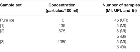
TABLE 1. The concentration of each solution created for the experiment. MI: Microsphere ice; UPI: Ultrapure ice; BI: Bottle isolate.

An additional ten 100 ml samples of liquid solutions [2] and [3] (Table 1), five samples of each solution, were prepared as control samples to test the reliability of the initial concentration of each solution and to test the recovery/loss in discrete samples. They were prepared directly inside new low-density polyethylene (LDPE; Nalgene™) bottles (BI), and stored sealed under controlled temperature conditions (+4°C).

Microsphere Sample Analysis

MI and UPI samples were melted using a Continuous Flow Analysis (CFA) system (Röthlisberger et al., 2000) in the ice chemistry lab at the British Antarctic Survey, United Kingdom. The sampling strategy was to complete sample runs where a single MI sample was first melted and then followed by three rinsing cycles with the meltwater from UPI samples (Figure 1; Table 1). All meltwater was split in the CFA melt plate into five 2-m long channels with identical Perfluoroalkoxy alkanes (PFA) tubing (internal diameter: 1.58 mm), where 40% of the meltwater went into a central “sample line” channel (SL), and the 60% left went randomly into four “waste line” channels (WL) at the sides of the melt plate. Meltwater was pumped using two Ismatec™ IPC digital peristaltic pumps, one for the SL and one for the four WL. Meltwater from the WL and SL was pumped through Polyvinyl chloride (PVC) tubing (internal diameter: 3.17 mm) at 2.5 rpm and 5 rpm, respectively. Meltwater at the end of the SL was directly filtered through 13 mm diameter, 1.0 μm pore size Whatman™ Polycarbonate membrane filter, inside clean polypropylene Swinnnex™ filter holders. Meltwater at the end of the WL was bottled into new low-density polyethylene (LDPE; Nalgene™) bottles, then pumped at 10 rpm (using the same pumps and tubing detailed above) and filtered with the same type of filter and holder used for the SL. After filtering each MI and UPI sample from the WL, sample bottles were rinsed three times with 100 ml of Milli-Q™ water, and all rinsing water was then filtered through the sample filter. During the CFA sampling, filters, filter holders and bottles were changed after every 100 ml ice strip was completely melted and the tubing was empty of meltwater.

FIGURE 1

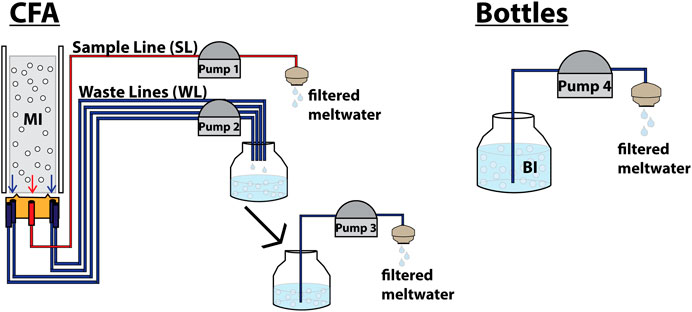
FIGURE 1. Schematic illustration of the experimental setup designed for this work. After filtering BI (100 ml) and after melting and filtering MI (100 ml), the same procedure was repeated three times with 100 ml ultrapure ice (UPI-1, UPI-2, and UPI-3) for MI and with 100 ml ultrapure water for BI. This was done to check for residual microspheres left in the tubing.

Additionally, BI samples were filtered under the same clean setup previously described (Figure 1). After filtering each sample, bottles were filled and rinsed three times with 100 ml Milli-Q™ water. After each rinsing cycle, the rinsing water was filtered.

All filters were mounted onto aluminum stubs for analyses on a Scanning Electron Microscope (SEM) at the Earth Sciences Department of the University of Cambridge. The entire filters were imaged on a Quanta-650F using Back Scattered Electrons (BSE) on a low-pressure mode. Each filter was imaged at ×200 magnification for microsphere identification and counting. The area of each 13 mm diameter filter comprised 16 transects; each transect was counted and the subtotals for each transect were tallied and divided by 16 to calculate the actual mean microsphere density per transect. To optimize the counting method, a Monte Carlo Simulation was used to determine the number of transects required to achieve a representative count. In this simulation X number of random transects were selected, the Monte Carlo Simulation divided the slide into X similar-sized groups of transects with one transect randomly selected from each group to promote greater coverage across the slide, the actual microsphere counts for the respective transects were summed and then divided by X to give a simulated microsphere density. For values of X from 1 to 8 this calculation was repeated up to 10,000 times for each filter. Results for each X value were plotted to create a progression curve. Then, progressions for each filter were averaged to obtain a mean progression curve (Allen et al., 2020).

Microsphere Loss Estimation

Microsphere loss was defined as the average deviation between microspheres recovered from each sample and the microspheres expected to be present in that sample (Table 1). To estimate potential microsphere losses throughout the method, each of the processes prone to produce losses was evaluated (Figure 1). These processes were identified as: pumping meltwater from bottles to filters, melting and transporting of the meltwater through the CFA system, and sample preparation process (together with the microsphere stock uncertainty). To estimate the loss, it was assumed that the only difference between SL samples and WL samples was the meltwater pumping process (Figure 1). Additionally, it was assumed that all samples were equally affected by losses associated with the sample preparation process (such as microsphere rejection while freezing, microsphere breaking while freezing, potential minor variations in the initial volumes pipetted from the stock, among others) and the microsphere stock uncertainty (SPMS). Loss estimations were calculated using the following equations:

$Pump losses (\%)= average BI recovery (\%) - average WL recovery (\%)(1)$

$SPMS losses (\%) = 100(\%) - average BI recovery (\%) - pump losses (\%)(2)$

$CFA losses (\%) = 100 (\%) - average SL recovery (\%)- SPMS losses (\%)(3)$

Ice Core Samples

To assess the performance of the standard method presented in this paper, targeted LC-IPM were analyzed in ice core samples following the sampling strategies detailed in section Discussion.

Ice samples from three Antarctic Peninsula (AP) ice cores (Jurassic, Rothschild and Smyley), provided by the British Antarctic Survey (BAS), were analyzed. The locations of these ice cores are shown in Figure 2 with the site information summarized in Table 2.

FIGURE 2

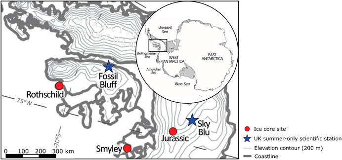
FIGURE 2. Map showing the ice core sites considered in this study. The red circles show the locations of the three ice core sites. The blue stars show the location of two United Kingdom summer-only scientific stations as reference.

TABLE 2

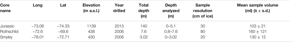
TABLE 2. Summary of each ice core geographical location and main features of the datasets analyzed in this study.

Ice core samples were cut into longitudinal sections using a band-saw with steel blade in the cold laboratory facilities at BAS. The Jurassic ice core samples for IPM analysis were obtained from the WL discharge from the CFA. The WL meltwater was collected in new low-density polyethylene (LDPE; Nalgene™) bottles at 30 cm of ice resolution. The Rothschild and Smyley ice core samples were cut and bottled, and then the sealed bottles were melted inside a fridge at 4°C. Once melted, all samples were treated to remove organic remains. Between 15 ml and 102 ml of 34% Hydrogen peroxide was added to create a 6% solution and left overnight in a warm bath at 60°C. After this, all samples were filtered through 13 mm diameter Whatman™ Polycarbonate membrane filters, with pore size 1.0 μm, inside pre-cleaned polypropylene Swinnnex™ filter holders. Filters were mounted onto aluminum stubs and then imaged on the same SEM detailed in section Laboratory Experiment. Filters were imaged at ×800 magnification for diatom identification, counting and classification, following the analysis strategies recommended in section Sample Analysis Strategy. Filters were analyzed for diatom identification as a real case study of LC-IPM analysis in ice core samples. Duplicates were performed in Rothschild ice core samples to test the reproducibility of the method. Eight sample bottles from the Jurassic and Smyley cores were subjected to additional rinsing cycles with ultrapure water. Rinsing water was filtered and filters were imaged (following the same procedure previously described) to test the effective removal of diatoms from the bottles and the system. Diatom identification and ecological associations were based on Armand et al. (2005), Hasle et al. (1996), Cefarelli et al. (2010), Zielinski and Gersonde (1997) and references therein. Ecological associations were determined for the most abundant species of each core. The assemblage composition was determined from the species with abundances higher than 2.0% of the whole assemblage.

Measurements of Methane sulfonic acid (MSA) were used to estimate the temporality of each ice core record. The MSA record was used as it has demonstrated to present a clear seasonal cycle in Antarctic ice cores, with a broad winter trough and a sharp austral summer maximum (Abram et al., 2013). Discrete ice samples were cut at 10 cm resolution and analyzed in a class-100 clean laboratory using a reagent free Dionex IC-2500 anion system.

Data from the ECMWF ERA5 reanalysis (Hersbach and Dee, 2019) were used to estimate mean precipitation (surface total precipitation parameter in ERA5) at each site. A recent study confirmed the high accuracy of ERA5 in representing the magnitude and variability of near-surface air temperature and wind regimes (Tetzner et al., 2019). Values reported in this work correspond to the annual mean precipitation of the decade before each ice core was drilled. The ERA5 reanalysis extends back to 1979, providing hourly data and at a 0.25° (∼31 km) resolution.

Results

Microspheres

Fourteen CFA runs were completed (MI sample followed by three rinsing cycles of UPI), producing 96 filters. Ten bottle runs were completed (BI sample followed by three rinsing cycles of 100 ml of ultrapure water) producing 40 filters. On each CFA and bottle run, microspheres were recovered and counted from SEM images. Table 3 presents the main results and the basic statistics of the filters analyzed. Table 4 shows the relation between the expected microsphere counts and the results obtained in the experiment.

TABLE 3

TABLE 3. Summary of the statistics of particle recovery. n = number of samples averaged. RSE: Relative Standard Error. (*): Concentrations refer to values presented in Table 1.

TABLE 4

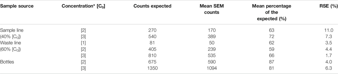
TABLE 4. Comparison between expected microsphere content and microsphere counts obtained from filters analyzed in SEM. RSE: Relative Standard Error. (*): Concentrations refer to values presented in Table 1.

Microsphere Reliability Test

Filters from bottle runs were analyzed to estimate the accuracy of the expected initial microsphere concentration (Table 1). Total counts from the ten runs presented on average 84% ± 4% of the expected initial microsphere concentration, values ranging from 71% to 102%. The discrepancies obtained between the expected counts and the SEM counts were independent (i.e., not proportional) of the initial concentration of microspheres on each sample (Table 4). The screening of the filter showed only microspheres, with no presence or signs of contamination.

Microsphere Recovery

The largest number of microspheres are recovered from the sample filters (MI and BI) as summarized in Table 3. There is a consistent exponential decay in the microsphere counts when transitioning from the sample filters (SL, WL, and BI) to the rinsing cycles (UPI series) (Figure 3), regardless of the sample type, microsphere concentration or the initial sample volume. Despite all exhibiting the same trend, decay is faster for samples collected from the CFA (SL and WL) than samples collected directly from bottles (BI). A common feature is a sharp decay in the microsphere counts to percentages below 1% of the total particulate material after UPI-1.

FIGURE 3

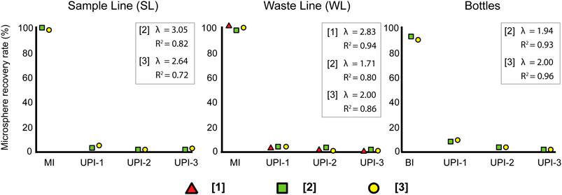
FIGURE 3. Mean trends of microsphere recovery rates from each sample source. Red triangles represent results obtained from low-concentration samples [1], green squares show results obtained from mid-concentration samples [2] and yellow circles show results from high-concentration samples [3]. λ: exponential decay constant.

There are considerable discrepancies when comparing the total number of microspheres counted on the SEM to the predicted number of microspheres on each run (Table 4). SEM microsphere counts are lower than the expected number of microsphere for each sample. The largest discrepancies are associated with the samples collected from the CFA. Microsphere counts in these samples exhibited a consistent average of 65% ± 3% of the expected initial microscope concentration (Tables 1 and 4). The magnitudes of the CFA disparities showed minor variations depending on the sample source (SL = 67.5% ± 6.6%; WL = 62.3% ± 2.0%) and no clear trend associated to the initial concentration of microspheres on each sample set.

Microsphere Loss Estimation

Microsphere losses were estimated on each of the processes performed while applying the method. The highest loss was associated with the preparation of the CFA strips, and the melting and transport of the meltwater through the CFA (21.7% ± 10.2%). Conversely, the lowest loss was associated with the pumping process (5.2% ± 6.9%). The loss associated with sample preparation processes and the microsphere stock uncertainty (SPMS) was estimated to be 10.8% ± 7.8%. Additionally, the loss of each sampling source was estimated (independent of the SPMS). For samples recovered from SL and BI, their losses correspond to the CFA (21.7% ± 10.2%) and to the pumping process (5.2% ± 6.9%), respectively. The loss for samples recovered from the WL is estimated to be the coupled loss from the CFA and the pumping process (26.9% ± 12.3%).

Microsphere Distribution

On each of the thirty-four sample filters, microspheres were counted in transects and subtotals for each transect were tallied to reflect the distribution of microspheres across the whole sample. Microsphere counts per transect were transformed onto a percentage of the total filter count. Transect percentages from all of the sample filters were used to calculate mean values per transect to determine the mean percentage contribution of each transect to a whole filter.

The mean microsphere percentage per transect profile shows a “plateau-shaped” distribution, where the central plateau extends between the fourth and 13th transect (Figure 4). This filter area presents a quasi-uniform distribution with a mean value (Relative standard error (RSE)) of 8.75% (±0.62%), representing 87.5% of the total counts in the filter. Conversely, transects beyond the plateau section (transects 1 to 3 and 14 to 16) present a sharp exponential decay toward the outer transects of the filter. These outer areas present a mean value (RSE) of 2.05% (±0.33%) and represent 12.5% of the total counts in the filter.

FIGURE 4

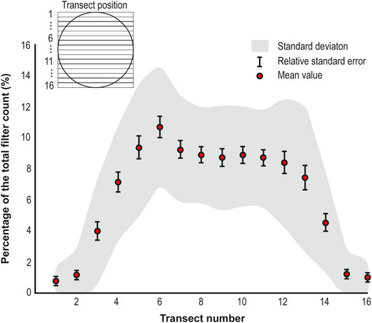
FIGURE 4. Mean microsphere percentage per transect profile and transect spatial distribution.

A Monte Carlo simulation was run to determine the optimum number of transects required to achieve representative counts, using transect counts from the thirty-four sample filters. Given their small contribution to the total counts, transects outside the plateau section were excluded from the simulation. The Monte Carlo simulation showed an increase in the representativeness of the counts (p) with the number of transects counted (n) (Figure 5). There is a steady increase in p until n = 3 (p = 99.7%, Stdev: ±11.327%, RSE: ±1.9%), when p stabilizes at ≈99%. Even though p becomes stable, the standard deviation of p shows a minor decreasing trend until n = 8.

FIGURE 5

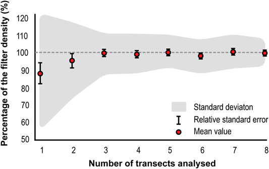
FIGURE 5. Monte Carlo simulated microsphere density per number of transects analyzed. Gray dashed line indicates the 100% limit.

Discussion

Microsphere Extraction, Loss and Recovery

The study of LC-IPM in ice samples requires a standardized method capable of recovering all the material present in the initial samples to ensure consistency and accuracy of the results. Our experiments to extract and recover microspheres from ice samples have shown consistent trends but slightly different levels of performance depending on the procedure used.

Extraction and Loss

An interesting result is the considerable discrepancy between the number of microspheres counted and the expected number of microspheres on each run. The calculated difference between the percentages recovered on the bottle runs (x̄ = 84% ± 4%) and on the CFA runs (x̄ = 65% ± 3%), implies major microsphere losses in the CFA system. This is confirmed by loss estimation, which presents the CFA as the main source of loss in the method (21.7% ± 10.2%). However, the absence of a cumulative increase in the counts from each CFA run (and the consistently low returns on the rinsed samples (UPI)) rules out the possibility of large numbers of microspheres getting lodged or temporally trapped in the CFA melt plate or inside the peristaltic pump system. Therefore, we suggest only a minor fraction of the missing microspheres is temporally trapped inside the CFA system. A major fraction could be potentially lost during the CFA sample preparation (MI) and/or during sample handling (minor scraping off uneven surfaces before loading the ice sample on the CFA). In particular, we propose that many microspheres could be fragmented during the sample freezing (a process not recommended by Polysciences, Inc., the manufacturer of Polybead^® Microspheres) and lost while filtrating or that some fragments were ignored during SEM scanning. If the effects of freezing are pervasive, microsphere fragmentation could account for a considerable fraction of the CFA losses, a loss not accounted in the SPMS loss estimation (Eq. 2). Either way, our preliminary estimation sets an upper threshold for a CFA loss estimation.

Similar losses have been previously reported in methods designed to extract and recover pollen from ice samples (Brugger et al., 2018). In particular, our CFA microsphere loss estimation is consistent with particle losses reported in filtration-based methods to recover pollen from ice cores (24%) (Short and Holdsworth, 1985; Brugger et al., 2018). Moreover, our method presents an equivalent performance to the best performing method designed to extract and recover pollen (22.1%) (Brugger et al., 2018). However, it must be acknowledged that our results are based on the performance of microspheres as analogues of real LC-IPM. Thus, the analysis of real LC-IPM could have higher or lower losses than those found in our experiments.

Previous studies have used polystyrene particles as standards to calibrate instruments or to test particle recovery (Wu et al., 2009; Ellis et al., 2015; Simonsen et al., 2018). However, their analyses have been limited to qualitative observations, instead of a percentile loss/recovery approach. Thus, the loss found here to be caused by sample preparation processes and microsphere stock uncertainty (10.8% ± 7.8%) provides a first quantitative estimate of the concentration uncertainty. Our loss estimation is in close agreement with the uncertainties reported in other particle markers (Lycopodium: 7%, Brugger et al., 2018). However, future experiments should be performed to determine the uncertainty of microsphere concentrations accurately when they are used in solutions as tracers.

Overall, our preliminary loss estimations provide a first approach to quantify the particles that are effectively reaching sample filters or CFA detectors traditionally used to analyze dust (Abakus, Coulter-Counter). Additionally, estimating the loss on each of the processes involved in the method allows comparing datasets obtained with different methods (continuous analysis (CFA) vs. discrete analysis (bottles)).

Recovery

Results from the SEM analyses have shown that despite the losses discussed in section Extraction and Loss, most of the recoverable fraction of microspheres is retrieved directly after filtering the sample (>90.3% ± 1.2%). Nevertheless, a small fraction of microspheres remains inside the tubing, even after the end of sample pumping (before the rinses). In particular, our results show that transporting and removing microspheres from a peristaltic pump system follows a consistent exponential decay trend. This trend indicates the existence of processes that hinder the transport of particles from the ice sample to the sample filter. A possible explanation for this exponential trend is the eventual lodging of a minor percentage of microspheres inside the tubing due to surface roughness or turbulence between the flow and the inner walls of the tubing. Our results are consistent with previous studies from related fields. In particular, exponential decay trends have been identified in studies related to the cleanout of residues from tanks and pipes (Fan, 2014; Osborne et al., 2015).

The exponential trend has important implications for successive sample processing, depending on the sampling setup. On the one hand, discrete sampling leaves behind up to 9.7% ± 0.6% of the particles after filtering the sample and underestimates the number of particles in the original ice sample. However, the exponential trend guarantees that remnants are almost entirely removed after one rinsing cycle, leaving behind less than 0.9% of the recoverable particles. Therefore, we recommend including at least one rinsing cycle (100 ml of Milli-Q™) to ensure more than 99% of the particles are collected in the sample filter. On the other hand, continuous sampling in a CFA system will produce a “memory effect” that will be passed through consecutive samples. Even though the memory effect in the SL will be negligible (<0.5% ± 0.2%), the memory effect in the CFA WL must be considered as it can reach up to 2.8% ± 1.1%. The extent of the memory effect will ultimately depend on the sampling resolution. The trend observed in our experiment demonstrates that WL samples with a sampling resolution of less than 10 cm of ice will produce a bias of >1.5% ± 0.4% in the consecutive sample. The effect on subsequent samples could be considered as negligible (<0.8% ± 0.2%). Therefore, we recommend 10 cm (≈100 ml) as a minimum threshold for sampling resolution with this method, mainly to ensure the memory effect is only affecting the consecutive sample. Additionally, if sampling firn, the sampling resolution must consider changes in the volume of meltwater transported by the WL due to the increase in density with depth. Memory effects, similar to the one previously described, have already been identified in CFA systems (Du et al., 2018).

Our results provide initial evidence of particle loss after the samples have been completely pumped through. This evidence suggests that dust (or LC-IPM) records could be slightly biased.

Sampling Recommendations

Based on our experimental results, we suggest different sampling strategies depending on the concentration of the targeted LC-IPM to be analyzed, the amount of ice available to sample, the sampling resolution and the time efficiency. The CFA SL has been shown to give the best performance to recover LC-IPM from ice samples. However, in a traditional ice core CFA campaign, meltwater from the SL is split into several detectors, reducing significantly the total volume of undisturbed meltwater that can be sampled (<20% of the initial SL volume). Even though the CFA SL presents the best performance, the final volume of water will become a limitation for CFA SL-derived LC-IPM analyses. We recommend that the SL is used only if the targeted LC-IPM is highly concentrated or if the sampling resolution is coarse enough to produce a significant volume of water to filter.

If the initial concentration of the targeted LC-IPM is low, we recommend sampling meltwater either from discrete LDPE bottles or from the CFA WL, depending on the availability of ice to sample. If ice is limited, we recommend sampling the meltwater from WL during a CFA campaign, reusing meltwater that otherwise would be discarded. However, sample bottles must be rinsed at least once and there will be a constant memory effect that must be acknowledged. Additionally, when sampling from the CFA WL, the abundance and diversity of the targeted LC-IPM must be assessed due to the potential contamination from the outer parts of the longitudinal CFA ice core samples. Alternatively, if ice is not limited or if the use of a CFA is not possible, we recommend creating discrete samples by cutting and bottling ice for subsequent melting and filtering. This sampling strategy will still require sample bottles to be rinsed at least once, but without the need to correct for a memory effect. However, it must be acknowledged that this method will be the slowest and possibly unfeasible for processing a large number of samples.

Sample Analysis Strategy

There is need to develop an optimized strategy for the analysis of LC-IPM samples, which traditionally is time-consuming. For this, first, it is necessary to determine how LC-IPM are distributed in sample filters. The mean microsphere distribution profile obtained from the sample filter counts shows a homogenous distribution of the material in the central area of the filter. Even though the material is distributed homogenously, the standard deviation of the central transects suggests that the analysis of a single transect could lead to significantly biased results. Results from the Monte Carlo simulation showed the analysis of three central transects (≈25% of the filter area and ≈26% of the material in the filter) produced the most representative results, with no significant improvements in the representativeness over this number. The optimum number of transects to analyze to obtain accurate results is three (99.7%, Stdev: ±11.3%, RSE: ±1.9%). Compared to other methods, this strategy presents a substantial reduction in the analysis time and more than two-fold increase in the area of the sample covered (Budgeon et al., 2012; Allen et al., 2020). Additionally, the considerable increase in the area covered by this strategy provides a more accurate representation of the diversity of material present on each sample (Allen et al., 2020). Altogether, these findings present an optimized strategy to study LC-IPM in filters, without the need to analyze the whole sample to get representative results. However, these estimations will have a 1.9% relative standard error associated with randomly selecting three transects from the central area of the filter. The error percentage in this analysis strategy is comparable to errors calculated from dust analysis techniques such as Laser particle detection-Abakus (<10%) (Ruth, 2002; Simonsen et al., 2019) and Coulter Counter (5%) (Simonsen et al., 2019).

Microspheres are a useful material for studying the behavior of particles and to calibrate instruments. However, their perfectly spherical shape do not accurately represent the morphological diversity present in IPM (Lambert et al., 2008; Simonsen et al., 2018). This highlights the need to validate our experimental results with real LC-IPM samples.

A Case Study: Diatoms in Ice Core Samples

Diatom Analyses

Thirty-five ice core samples were analyzed following the recommendations and strategies presented in section Discussion. A total of 1,424 diatoms valves and fragments were found among all samples. There was an increasing trend in the mean diatom size from coastal to inland sites (Figure 2), ranging from 9.1 µm (Rothschild) to 21 µm (Jurassic). Identifiable diatoms were classified based on their genus level or higher. Diatoms were well preserved, without evidence of dissolution in their ornamentation (Warnock and Scherer, 2015). Ecological affinities of the identified diatom taxa indicate an almost exclusively marine assemblage, largely dominated by Fragilariopsis spp. and Thalassiosira spp., two abundant genus in the Southern Ocean. Even though diatom assemblages show variations in the AP ice cores, results are consistent in showing that Fragilariopsis cylindrus is the most abundant diatom species across all three ice core sites (Figure 6). The observed diatom diversity suggests the seasonal sea-ice zone as the likely dominant diatom source (Pike et al., 2008; Esper and Gersonde, 2014). This agrees with regional atmospheric circulation showing that most air masses reaching the ice core sites on the AP travel over the Bellingshausen Sea and the English coast (Thomas and Bracegirdle, 2015), areas with the consistent presence of winter and summer sea ice (Abram et al., 2013). Our results agree with previous studies showing the wide presence of marine diatoms in snow and ice samples from the Antarctic ice sheet (Kellogg and Kellog., 1996; Budgeon et al., 2012; Allen et al., 2020).

FIGURE 6

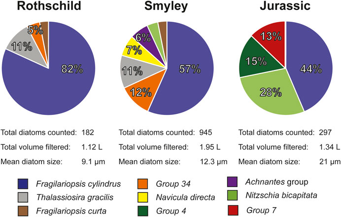
FIGURE 6. Main diatom ecological associations obtained from each of the AP ice cores. Percentages reported in this figure were normalized to the main species present on each core. Group 4, Group 7, and Group 34, each corresponds to a particular diatom species that was not identified.

The AP ice cores differ in their mean diatom abundance. The Jurassic and Rothschild ice cores present similar mean diatom abundance values, while the Smyley core presents considerably higher values (Figure 7). Mean diatom abundances in the AP cores appear to be comparable with results obtained from Wilkes Land (0–180 L⁻¹) and Ellsworth Land (0–140 L⁻¹) (Budgeon et al., 2012; Allen et al., 2020). The diatom abundance depth-profiles show regular sinusoidal short-scale variations down-core (Figure 7). This evidences that the effective deposition and burial of diatoms in the snow is not a constant feature. The ERA5 reanalysis estimates that the mean precipitation rates in Rothschild, Smyley and Jurassic are 95.9, 98.5, and 101.8 cm of water equivalent per year, respectively. Based on reanalysis estimates and MSA concentration profiles, the short scale-variations identified down-core could be indicative of significant inter-annual and intra-annual variations in the diatom deposition. In particular, considering the presence of sharp summer MSA peaks and the slight underestimation in ERA5 precipitation (Tetzner et al., 2019), it is likely that short-scale variations in the diatom record are indicative of intra-annual variations. Inter-annual variations in the ice core diatom record have already shown the potential to be a proxy of wind strength (Allen et al., 2020). However, if the variations seen in the AP cores are also representative of seasonal changes, the diatom record in ice cores could hold the potential to be used as an independent seasonal marker within ice core chronologies. Furthermore, if the diatom record is seasonal, the inter-annual wind proxy could be biased by this effect.

FIGURE 7

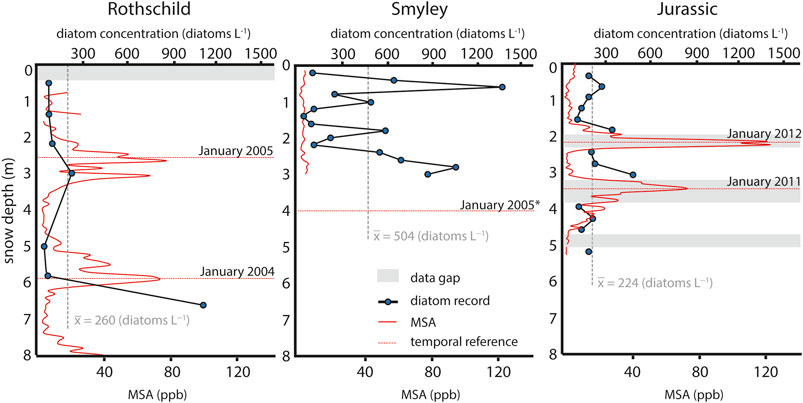
FIGURE 7. Diatom abundance variations down-core and MSA concentration profiles. Gray dashed line indicates the mean diatom abundance on each core. Gray bands indicate data gaps. Red dashed line indicates temporal horizons based on the austral summer maxima in MSA. (*) Temporal horizon estimation based on the record of a 4-metre Automatic Weather Station installed in Smyley in January 2005 and completely buried under the snow by January 2006.

The method presented in this work provides an effective way to recover and analyze diatoms from ice core samples. The high abundance of diatoms in the AP cores, the proximity of their source and the significant variations seen in the depth profiles highlight the potential of these records to provide valuable climate information.

Method Validation

Three tests were conducted in the AP ice core samples to evaluate the performance of the method. To test the reproducibility of the method, duplicates from the Rothschild ice core were analyzed. Duplicates were created covering the same depth and the same water volume. Duplicate diatom counts and diatom abundance show a high degree of correspondence with the original samples (R²= 0.99, p < 0.01) (Figure 8). Even though duplicate counts are slightly higher than the original counts (+8.8%), this magnitude remains within the ±11.3% standard deviation margin predicted by the filter analysis strategy presented in section Sample Analysis Strategy. Additionally, duplicate analyses present a strong agreement with the mean diatom size and the diatom diversity observed in the original sample (Figure 8).

FIGURE 8

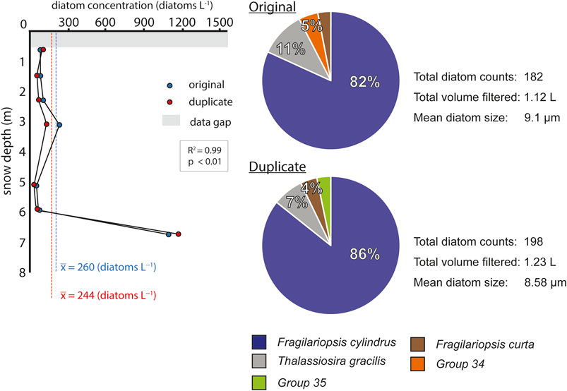
FIGURE 8. Rothschild duplicates. Diatom abundance variations and main diatom associations obtained from the original Rothschild core and the duplicate. Blue dashed line indicates the mean diatom abundance of the original Rothschild core. Red dashed line indicates the mean diatom abundance of the duplicate Rothschild core. Group 34 and Group 35, each corresponds to a particular diatom species that was not identified.

To test the efficiency of removing material from the system, six sample bottles were rinsed for a second and a third time. After each rinsing, water was filtered to scan for the presence of remaining material in the system. Only two diatoms were found in the second rinsing cycle of the 0.4 and 0.6 m-deep samples from the Smyley core. These samples originally yielded 79 and 142 diatom counts, respectively. The presence of one diatom in each sample after a second rinsing cycle agrees with the magnitude predicted by the exponential decay observed in section Microspheres.

To test the consistency in the distribution of particles in the central transects (4th–13th) of the filters (Figure 4), diatom counts per transect were recorded on each filter to determine a mean distribution. Mean values (RSE) show that each of the three central transects holds 36% (±3%), 30% (±2%) and 34% (±3%) of the diatoms counted on each filter. The uniformity of the mean values and the percentile fraction of their relative standard errors match the mean distribution profile presented in section Microsphere distribution.

Studying the presence of diatoms in ice cores has provided a real case study to test the experimental results of our standard method. Even though some studies have cataloged microspheres as unrealistic for this purpose (Simonsen et al., 2018), our experimental results have shown that our proposed method accurately predicts the analytical precision of recovering diatoms from ice samples, validating the use of microspheres for this kind of analyses. These results highlight the potential of our standard method to be applied in the study of other LC-IPM’s in ice cores. Adaptations to our standard method may be necessary when it is applied to different kinds of LC-IPM.

Conclusion

The study of LC-IPM in ice has provided distinctive and valuable information to study the Earth’s past climate. A new standard method to sample, recover and analyze LC-IPM from ice samples has been tested in discrete and continuous analysis setups. Both setups are effective in recovering particles from the sample with quantifiable particle losses. More than 90% of the particles is directly recovered after filtering. The removal of the remaining fraction of the sample follows an exponential decrease trend, with more than 99% of the sample recovered after rinsing the system. This trend predicts a memory effect of up to 2.8% in samples retrieved from the continuous analysis setup.

Particles recovered from the sample present a homogeneous distribution in the sample filters. A statistical analysis of their distribution determined that the analysis of 25% of the filter area lead to representative results (99.7% ± 1.9%). Thus, this procedure optimizes the estimation of particle abundance and diversity.

This method was tested and validated using diatoms in ice cores. The results show a particularly high abundance of diatoms, a traceable marine source and significant variations down-core. Altogether, this demonstrates the existence of a valuable record for future research on past climate, uncovering the high potential of the diatom record from Antarctic Peninsula ice cores.

Overall, the new optimized method presented in this work has demonstrated itself to be effective at extracting, recovering and analyzing micrometre-sized LC-IPM to obtain statistically representative results. This standard method offers the opportunity to produce robust quantitative studies of LC-IPM in samples directly extracted from a CFA. Additionally, the systematic assessment of the method reveals consistent and quantifiable particle loss that most likely reflects the underestimation of the raw microsphere concentration and reveals that a single rinse after sample extraction ensures a >99% extraction.

Data Availability Statement

The raw data supporting the conclusions of this article will be made available by the authors, without undue reservation.

Author Contributions

Conceptualization, DT, ET, and CA; methodology, DT and CA; formal analysis, DT, ET, CA, and EW; investigation, DT; Writing—Original Draft preparation, DT; Writing—Review and Editing, DT, ET, CA, and EW.

Funding

This research was funded by CONICYT–Becas Chile and Cambridge Trust funding program for PhD studies. Grant number 72180432.

Conflict of Interest

The authors declare that the research was conducted in the absence of any commercial or financial relationships that could be construed as a potential conflict of interest.

References

Abram, N. J., Wolff, E. W., and Curran, M. A. J. (2013). A review of sea ice proxy information from polar ice cores. Quat. Sci. Rev. 79, 168–183. doi:10.1016/j.quascirev.2013.01.011

CrossRef Full Text | Google Scholar

Allen, C. S., Thomas, E. R., Blagbrough, H., Tetzner, D. R., Warren, R. A., Ludlow, E. C., et al. (2020). Preliminary evidence for the role played by South Westerly wind strength on the marine diatom content of an Antarctic Peninsula Ice Core (1980–2010). Geosciences 10 (3), 87. doi:10.3390/geosciences10030087

CrossRef Full Text | Google Scholar

Alley, R. B. (2010). Reliability of ice-core science: historical insights. J. Glaciol. 56 (200), 1095–1103. doi:10.3189/002214311796406130

CrossRef Full Text | Google Scholar

Alley, R. B. (2014). The two-mile time machine: ice cores, Abrupt climate change, and our future-updated edition (Princeton: Princeton University Press), Vol. 31.

Armand, L. K., Crosta, X., Romero, O., and Pichon, J. J. (2005). The biogeography of major diatom taxa in Southern Ocean sediments: 1. Sea ice related species. Palaeogeogr. Palaeoclimatol. Palaeoecol. 223 (1–2), 93–126. doi:10.1016/j.palaeo.2005.02.015

CrossRef Full Text | Google Scholar

Baccolo, G., Cibin, G., Delmonte, B., Hampai, D., Marcelli, A., Di Stefano, E., et al. (2018). The contribution of synchrotron light for the characterization of atmospheric mineral dust in deep ice cores: preliminary results from the talos dome ice core (east antarctica). Condens. Matter. 3 (3), 25. doi:10.3390/condmat3030025

CrossRef Full Text | Google Scholar

Bourgeois, J. C., Koerner, R. M., Gajewski, K., and Fisher, D. A. (2000). A holocene ice-core pollen record from Ellesmere Island, Nunavut, Canada. Quat. Res. 54 (2), 275–283. doi:10.1006/qres.2000.2156

CrossRef Full Text | Google Scholar

Brugger, S. O., Gobet, E., Blunier, T., Morales-Molino, C., Lotter, A. F., Fischer, H., et al. (2019). Palynological insights into global change impacts on Arctic vegetation, fire, and pollution recorded in Central Greenland ice. Holocene 29 (7), 1189–1197. doi:10.1177/0959683619838039

CrossRef Full Text | Google Scholar

Brugger, S. O., Gobet, E., Schanz, F. R., Heiri, O., Schwörer, C., Sigl, M., et al. (2018). A quantitative comparison of microfossil extraction methods from ice cores. J. Glaciol. 64 (245), 432–442. doi:10.1017/jog.2018.31

CrossRef Full Text | Google Scholar

Budgeon, A. L., Roberts, D., Gasparon, M., and Adams, N. (2012). Direct evidence of aeolian deposition of marine diatoms to an ice sheet. Antarct. Sci. 24 (5), 527–535. doi:10.1017/s0954102012000235

CrossRef Full Text | Google Scholar

Cefarelli, A. O., Ferrario, M. E., Almandoz, G. O., Atencio, A. G., Akselman, R., and Vernet, M. (2010). Diversity of the diatom genus Fragilariopsis in the Argentine Sea and Antarctic waters: morphology, distribution and abundance. Polar Biol. 33 (11), 1463–1484. doi:10.1007/s00300-010-0794-z

CrossRef Full Text | Google Scholar

Cook, E., Portnyagin, M., Ponomareva, V., Bazanova, L., Svensson, A., and Garbe-Schönberg, D. (2018). First identification of cryptotephra from the Kamchatka Peninsula in a Greenland ice core: implications of a widespread marker deposit that links Greenland to the Pacific northwest. Quat. Sci. Rev. 181, 200–206. doi:10.1016/j.quascirev.2017.11.036

CrossRef Full Text | Google Scholar

Davies, S. M., Abbott, P. M., Pearce, N. J. G., Wastegård, S., and Blockley, S. P. E. (2012). Integrating the INTIMATE records using tephrochronology: rising to the challenge. Quat. Sci. Rev. 36, 11–27. doi:10.1016/j.quascirev.2011.04.005

CrossRef Full Text | Google Scholar

Delmonte, B., Winton, H., Baroni, M., Baccolo, G., Hansson, M., Andersson, P., et al. (2019). Holocene dust in East Antarctica: provenance and variability in time and space. Holocene 30, 0959683619875188. doi:10.1177/0959683619875188

CrossRef Full Text | Google Scholar

Du, W.-t., Kang, S.-c., Qin, X., Sun, W.-j., Zhang, Y.-l., Liu, Y.-s., et al. 2018). Review of pre-processing technologies for ice cores. J. Mt. Sci. 15 (9), 1950–1960. doi:10.1007/s11629-017-4679-2

CrossRef Full Text | Google Scholar

Dunbar, N. W., and Kurbatov, A. V. (2011). Tephrochronology of the Siple Dome ice core, West Antarctica: correlations and sources. Quat. Sci. Rev. 30 (13–14), 1602–1614. doi:10.1016/j.quascirev.2011.03.015

CrossRef Full Text | Google Scholar

Dunbar, N. W., Iverson, N. A., Van Eaton, A. R., Sigl, M., Alloway, B. V., Kurbatov, A. V., et al. (2017). New Zealand supereruption provides time marker for the Last Glacial Maximum in Antarctica. Sci. Rep. 7 (1), 12238. doi:10.1038/s41598-017-11758-0

PubMed Abstract | CrossRef Full Text | Google Scholar

Ellis, A., Edwards, R., Saunders, M., Chakrabarty, R. K., Subramanian, R., van Riessen, A., et al. (2015). Characterizing black carbon in rain and ice cores using coupled tangential flow filtration and transmission electron microscopy. Atmos. Meas. Tech. 8, 3959–3969. doi:10.5194/amt-8-3959-2015

Esper, O., and Gersonde, R. (2014). Quaternary surface water temperature estimations: new diatom transfer functions for the Southern Ocean. Palaeogeogr. Palaeoclimatol. Palaeoecol. 414, 1–19. doi:10.1016/j.palaeo.2014.08.008

CrossRef Full Text | Google Scholar

Fan, M. (2014). Effectiveness of pre-rinse during in-place cleaning of stainless steel pipe lines. PhD dissertation: Ohio: Ohio State University.

Google Scholar

Festi, D., Kofler, W., Bucher, E., Carturan, L., Mair, V., Gabrielli, P., et al. (2015). A novel pollen-based method to detect seasonality in ice cores: a case study from the Ortles glacier, South Tyrol, Italy. J. Glaciol. 61 (229), 815–824. doi:10.3189/2015jog14j236

CrossRef Full Text | Google Scholar

Hasle, G. R., Syvertsen, E. E., and von Quillfeldt, C. H. (1996). Fossula Arcticagen. nov., spec. nov., a marine Arctic araphid diatom. Diatom. Res. 11 (2), 261–272. doi:10.1080/0269249x.1996.9705383

CrossRef Full Text | Google Scholar

Hersbach, H., and Dee, D. J. E. N. (2019). ERA5 reanalysis is in production. ECMWF newsletter 147 (7), 5–6. doi:10.21957/vf291hehd7

Google Scholar

Kellogg, D. E., and Kellogg, T. B. (1996). Diatoms in South Pole ice: implications for eolian contamination of Sirius Group deposits. Geology 24 (2), 115–118. doi:10.1130/0091-7613(1996)024<0115:dispii>2.3.co;2

CrossRef Full Text | Google Scholar

Kellogg, D. E., and Kellogg, T. B. (2005). Frozen in time: the diatom record in ice cores from remote drilling sites on the Antarctic ice sheets. Princeton, NJ, United States: Princeton University Press, 69–93.

CrossRef Full Text

Lambert, F., Delmonte, B., Petit, J. R., Bigler, M., Kaufmann, P. R., Hutterli, M. A., et al. (2008). Dust-climate couplings over the past 800,000 years from the EPICA Dome C ice core. Nature 452 (7187), 616–619. doi:10.1038/nature06763

PubMed Abstract | CrossRef Full Text | Google Scholar

Legrand, M., and Mayewski, P. (1997). Glaciochemistry of polar ice cores: a review. Rev. Geophys. 35 (3), 219–243. doi:10.1029/96rg03527

CrossRef Full Text | Google Scholar

McConnell, J. R., Edwards, R., Kok, G. L., Flanner, M. G., Zender, C. S., Saltzman, E. S., et al. (2007). 20th-century industrial black carbon emissions altered arctic climate forcing. Science 317 (5843), 1381–1384. doi:10.1126/science.1144856

PubMed Abstract | CrossRef Full Text | Google Scholar

Nakazawa, F., and Fujita, K. (2006). Use of ice cores from glaciers with melting for reconstructing mean summer temperature variations. Ann. Glaciol. 43, 167–171. doi:10.3189/172756406781812302

CrossRef Full Text | Google Scholar

Osborne, P. P., Xu, Z., Swanson, K. D., Walker, T., and Farmer, D. K. (2015). Dicamba and 2,4-D residues following applicator cleanout: a potential point source to the environment and worker exposure. J. Air Waste Manag. Assoc. 65 (9), 1153–1158. doi:10.1080/10962247.2015.1072593

PubMed Abstract | CrossRef Full Text | Google Scholar

Osmont, D., Wendl, I. A., Schmidely, L., Sigl, M., Vega, C. P., Isaksson, E., et al. (2018). An 800-year high-resolution black carbon ice core record from Lomonosovfonna, Svalbard. Atmos. Chem. Phys. 18 (17), 12777–12795. doi:10.5194/acp-18-12777-2018

CrossRef Full Text | Google Scholar

Pike, J., Allen, C. S., Leventer, A., Stickley, C. E., and Pudsey, C. J. (2008). Comparison of contemporary and fossil diatom assemblages from the western Antarctic Peninsula shelf. Mar. Micropaleontol. 67 (3–4), 274–287. doi:10.1016/j.marmicro.2008.02.001

CrossRef Full Text | Google Scholar

Röthlisberger, R., Bigler, M., Hutterli, M., Sommer, S., Stauffer, B., Junghans, H. G., et al. (2000). Technique for continuous high-resolution analysis of trace substances in firn and ice cores. Environ. Sci. Technol. 34 (2), 338–342. doi:10.1021/es9907055

CrossRef Full Text | Google Scholar

Ruth, U. (2002). Concentration and size distribution of microparticles in the NGRIP ice core (Central Greenland) during the last glacial period. PhD dissertation. Bremen.

Google Scholar

Ruth, U., Wagenbach, D., Steffensen, J. P., and Bigler, M. (2003). Continuous record of microparticle concentration and size distribution in the central Greenland NGRIP ice core during the last glacial period. J. Geophys. Res.: Atmos. 108 (D3), 4098. doi:10.1029/2002jd002376

CrossRef Full Text | Google Scholar

Short, S. K., and Holdsworth, G. (1985). Pollen, oxygen isotope content and seasonally in an ice core from the penny Ice Cap, Baffin Island. Arctic 38, 214–218. doi:10.14430/arctic2136

CrossRef Full Text | Google Scholar

Sigl, M., Winstrup, M., McConnell, J. R., Welten, K. C., Plunkett, G., Ludlow, F., et al. (2015). Timing and climate forcing of volcanic eruptions for the past 2,500 years. Nature 523 (7562), 543–549. doi:10.1038/nature14565

PubMed Abstract | CrossRef Full Text | Google Scholar

Simonsen, M. F., Baccolo, G., Blunier, T., Borunda, A., Delmonte, B., Frei, R., et al. (2019). East Greenland ice core dust record reveals timing of Greenland ice sheet advance and retreat. Nat. Commun. 10 (1), 4494–4498. doi:10.1038/s41467-019-12546-2

PubMed Abstract | CrossRef Full Text | Google Scholar

Simonsen, M. F., Cremonesi, L., Baccolo, G., Bosch, S., Delmonte, B., Erhardt, T., et al. (2018). Particle shape accounts for instrumental discrepancy in ice core dust size distributions. Clim. Past 14 (5), 601–608. doi:10.5194/cp-14-601-2018

CrossRef Full Text | Google Scholar

Tetzner, D., Thomas, E., and Allen, C. (2019). A validation of ERA5 reanalysis data in the Southern Antarctic Peninsula-Ellsworth Land region, and its implications for ice core studies. Geosciences 9 (7), 289. doi:10.3390/geosciences9070289

CrossRef Full Text | Google Scholar

Thomas, E. R., and Bracegirdle, T. J. (2015). Precipitation pathways for five new ice core sites in Ellsworth Land, West Antarctica. Clim. Dynam. 44 (7–8), 2067–2078. doi:10.1007/s00382-014-2213-6

CrossRef Full Text | Google Scholar

Tison, J. L., de Angelis, M., Littot, G., Wolff, E., Fischer, H., Hansson, M., et al. (2015). Retrieving the paleoclimatic signal from the deeper part of the EPICA Dome C ice core. Cryosphere 9, 1633–1648. doi:10.5194/tc-9-1633-2015

CrossRef Full Text | Google Scholar

Vallelonga, P., and Svensson, A. (2014). “Ice core archives of mineral dust,” in Mineral dust (Dordrecht: Springer), 463–485.

CrossRef Full Text | Google Scholar

Warnock, J. P., and Scherer, R. P. (2015). A revised method for determining the absolute abundance of diatoms. J. Paleolimnol. 53 (1), 157–163. doi:10.1007/s10933-014-9808-0

CrossRef Full Text | Google Scholar

Wolff, E. W., Chappellaz, J., Blunier, T., Rasmussen, S. O., and Svensson, A. (2010). Millennial-scale variability during the last glacial: the ice core record. Quat. Sci. Rev. 29 (21–22), 2828–2838. doi:10.1016/j.quascirev.2009.10.013

CrossRef Full Text | Google Scholar

Wu, G., Zhang, C., Gao, S., Yao, T., Tian, L., and Xia, D. (2009). Element composition of dust from a shallow Dunde ice core, Northern China. Global Planet. Change 67 (3–4), 186–192. doi:10.1016/j.gloplacha.2009.02.003

CrossRef Full Text | Google Scholar

Zielinski, U., and Gersonde, R. (1997). Diatom distribution in Southern Ocean surface sediments (Atlantic sector): implications for paleoenvironmental reconstructions. Palaeogeogr. Palaeoclimatol. Palaeoecol. 129 (3–4), 213–250. doi:10.1016/s0031-0182(96)00130-7

CrossRef Full Text | Google Scholar