Analysis of Swarm Satellite Magnetic Field Data Before the 2016 Ecuador (Mw = 7.8) Earthquake Based on Non-negative Matrix Factorization

Introduction

Earthquakes are the most energetic phenomena in the lithosphere and on the Earth (Bolt, 1999). During the long-term earthquake preparation processing and at the largest energy release moment of earthquakes, some seismic-linked anomalies could occur in the lithosphere, atmosphere, and ionosphere (Parrot, 1995; Freund, 2000; Liu et al., 2015; Hattori and Han, 2018; Piscini et al., 2019). With the development of the Lithosphere–Atmosphere–Ionosphere Coupling (LAIC) model, the study of seismo-ionospheric anomalies has attracted more and more attention (Hayakawa and Molchanov, 2002; Pulinets and Ouzounov, 2011; De Santis et al., 2015, 2019a; Shen et al., 2018; Li et al., 2019; Fu et al., 2020; Zhima et al., 2020). Recently, a substantial amount of satellite observation data are used to study the ionosphere anomalies before large earthquakes (Pulinets and Boyarchuk, 2005; Ho et al., 2018; Natarajan and Philipoff, 2018; Marchetti et al., 2019c; Zhang et al., 2019).

Swarm is a satellite mission of the European Space Agency (ESA). The mission consists of three satellites (Alpha, Bravo, and Charlie) that are devoted to studying the geomagnetic field and its dynamics (Olsen et al., 2006; Bouffard et al., 2019). The magnetic field data of Swarm satellites are widely used in fields, such as studying the ionospheric current systems (Alken, 2016) and the magnetic storms (Wang et al., 2019), and constructing the magnetic field models (Finlay et al., 2015, 2016). Beyond this, the high-precision magnetic field data are also applied to study the ionosphere anomalies, which are possibly related to earthquakes (De Santis et al., 2019b; Marchetti et al., 2019a). After the launch of the Swarm satellites at the end of 2013, some large earthquakes occurred. We focused on the 7.8 Mw earthquake that occurred in Ecuador (0.35°N, 79.93°W) on April 16, 2016.

Since satellite magnetic field data are affected by geomagnetic activity (Zhima et al., 2014; Perrone et al., 2018), in the routine analysis of the anomalies of earthquakes, the data under strong geomagnetic conditions are usually deleted. Zhang et al. (2009) studied the 2007 Chile M7.9 earthquake using the DEMETER satellite magnetic field data with Kp < 3 and Dst > −20 nT and found that the low frequency electromagnetic disturbances increased 1 week before the earthquake. Akhoondzadeh et al. (2019) used the magnetic field data collected under quiet geomagnetic conditions to study the 2017 Sarpole Zahab (Mw = 7.3) earthquake and observed ionospheric magnetic anomalies between 8 and 11 days prior to the occurrence of the event. De Santis et al. (2019c) used the Swarm satellite magnetic field data with |Dst| ≤ 20 nT and a_p ≤ 10 nT to study 12 earthquakes with magnitudes from 6.1 to 8.3, and they observed some ionospheric magnetic field anomalies before most of the events (Yan et al., 2013; Marchetti and Akhoondzadeh, 2018; De Santis et al., 2019b; Marchetti et al., 2019a,b).

Hattori et al. (2004) applied the principal component analysis to decompose the magnetic field data of three ground-based stations (including the data under strong geomagnetic activity). The first and the second principal components were found to be associated with the geomagnetic variation and man-made activity, respectively, and the residual third component contained the earthquake precursory signature. Then, in 2019, the principal component analysis was applied to the satellite magnetic field data by Zhu et al. (2019); they removed the component, which has a high correlation coefficient with the a_p index, and extracted earthquake-related anomalies using the residual component.

Non-negative matrix factorization (Lee and Seung, 1999) is a parts-based matrix decomposition method that has the advantage of obtaining local features from the whole data, which differs from the principal component analysis. NMF has been successfully applied in various fields. Lee and Seung (1999) proposed NMF and applied the method to decompose face images into basis images, such as the mouth, the nose, and other facial parts. Smaragdis and Brown (2003) applied NMF to decompose complex piano music and obtained the spectral bases of each note and its weight in time. Mouri et al. (2009) applied NMF to decompose electromagnetic data with extremely low-frequency bands from multiple ground stations and obtained local signals (which are emitted by regional electromagnetic radiation sources) from the extremely low-frequency data. Since the impact of earthquakes occurs only near the epicenters. Based on the advantage of NMF that could obtain local features from the overall data, in this paper, we used the NMF to analyze the ionosphere magnetic field data of Swarm Alpha satellite, including the data collected under quiet geomagnetic conditions and those under strong geomagnetic conditions, to explore the 2016 Ecuador earthquake (April 16, 0.35°N, 79.93°W).

First, we briefly described the Swarm satellite magnetic field data and the NMF method. Next, we performed NMF to decompose the short-time Fourier transform (STFT) magnitude spectra of each track and obtained three basis features and their corresponding weights. We calculated the energy-entropy ratio of the three weight components. For the weight component with the highest energy-entropy ratio, we computed the cumulative number of tracks, which had anomalies inside the earthquake-sensitive area. In addition, we analyzed the influence of geomagnetic activity and plasma bubbles on the cumulative anomaly. From the random earthquake study and low-seismicity period study, we explored whether the cumulative anomaly was obtained by chance. Finally, we studied the correlation between the ionosphere magnetic anomaly and the lithosphere activity.

Data and Method

Swarm Satellite Magnetic Field Data

The Swarm mission consisted of three identical satellites (Alpha, Bravo, and Charlie), which had been launched into near-polar orbits on November 22, 2013 (Bouffard et al., 2019). The satellites, Alpha and Charlie, flew almost side-by-side (longitudinal separation of 1.4° at the equator) at an altitude near 462 km (initial altitude) and the Bravo flew higher, near 511 km (initial altitude). The three satellites completed one track in about 90 min, accomplished nearly 15 day-and-night passes every 24 h, and drifted about 1 h in local time (LT), every 10 days. The objective of the mission was to provide the best survey and the temporal evolution of the geomagnetic field, obtain a space-time characterization of the internal field sources in the Earth, while improving the understanding of the interior of the Earth and the Geospace environment (Friis-Christensen et al., 2006, 2008; Olsen et al., 2006).

Each satellite of the Swarm mission was equipped with seven instruments. The main sensors included two magnetometers, an Absolute Scalar Magnetometer that provided measurements of the field intensity, and a Vector Field Magnetometer that measured the magnetic field from three different directions. These sensors made high-precision and high-resolution measurements of the strength, direction, and variation of the magnetic field. The observations are provided as Level-1b data, which are then calibrated and formatted time series (Olsen et al., 2013).

The observation data of vector magnetic field in L1b products are shown in two reference systems: (1) the instrument frame and (2) the North (X) East (Y) Center (Vertical, Z) frame. The magnetic field of the Y-East component could be affected by lithospheric activity and is less influenced by external magnetic disturbances (Pinheiro et al., 2011). In this study, we analyzed the Y-East component magnetic field data (Level-1b 1 Hz data) of the Swarm Alpha satellite to study the 2016 Ecuador earthquake.

Non-negative Matrix Factorization

The non-negative matrix factorization (Paatero and Tapper, 1994; Lee and Seung, 2000; Smaragdis, 2004; Cichocki et al., 2006) is a matrix factorization algorithm that approximates a given non-negative matrix as a product of two other non-negative matrices. The two decomposed non-negative matrices consist of a few basis vectors which contain the potential structures of the given non-negative matrix. This algorithm can obtain parts-based representations of non-negative data and make no further assumptions about their statistical dependencies. Thus, NMF could obtain local features from the overall data.

The goal of NMF is to approximate the non-negative matrix V as a product of two non-negative matrices, W and H. The approximate factorization can be written as in Equation (1).

$\begin{array}{l}V\approx WH\\ \approx \begin{array}{c}[W_{*1}\cdots W_{*r}]\\ \end{array}\left[\begin{array}{c}{H}_{1*}\\ ⋮\\ H_{r*}\\ \end{array}\right]& (1)\end{array}$

where, V ∈ ℝ^{≥0, m×n} is the original matrix, W ∈ ℝ^{≥0, m×r} is the basis matrix, and H ∈ ℝ^{≥0, r×n} is the weight matrix. W_*1, …, W_*r are the columns of matrix W and can be interpreted as basis vectors of matrix V. H_1*, …, H_r* are the rows of matrix H, which have a one-to-one correspondence with the columns of W and can be interpreted as the weights of these basis vectors. The rank r corresponds to the number of basis vectors, and is generally selected, such that (n + m)r < nm.

To minimize the error of reconstruction of V by WH, we use the cost function based on the generalized Kullback–Leibler divergence. We constrained the solutions of NMF problems by the minimum determinant constraint (Schachtner et al., 2009), which could achieve unique and optimal solutions in a general setting. The cost function is shown in Equation (2).

$\begin{array}{l}{D}_{detKL}(V|W,H)={\displaystyle \sum _{i=1}^m}{\displaystyle \sum _{j=1}^n}\left(V_{ij}ln\frac{V_{ij}}{{\left[WH\right]}_{ij}}-V_{ij}+{\left[WH\right]}_{ij}\right)\\ +\alpha det\left(H{H}^T\right)& (2)\end{array}$

where, α is the balance parameter. When α remains small enough, the reconstruction error does not increase during an iteration step, and very satisfactory results are obtained.

To optimize this function, we used an efficient multiplicative update algorithm introduced by Lee and Seung (2000); the iterative updated rules of basis matrix, W and weight matrix, H are shown in Equations (3) and (4).

$\begin{array}{ll}W\leftarrow W\frac{\frac{V}{\left[WH\right]}{H}^T}{I{H}^T}& (3)\end{array}$

$\begin{array}{ll}H\leftarrow H\left(\frac{W^T\frac{V}{\left[WH\right]}}{W^{T}I}-\alpha det\left(H{H}^T\right)\frac{\left[{\left(H{H}^T\right)}^{-1}H\right]}{W^{T}I}\right)& (4)\end{array}$

We stopped the iteration when the D_detKL (V|W, H)is was smaller than the threshold Th or the number of iterations reached the upper limit, N_iter. The formula for calculating Th is shown in Equation (5).

$\begin{array}{ll}Th=\epsilon {\displaystyle \sum _{i=1}^m}{\displaystyle \sum _{j=1}^n}{V}_{ij}& (5)\end{array}$

where, ε is the error factor. This parameter should be a small value and set according to the actual needs.

Overall, the NMF algorithm can be summarized as follows:

1. Initialize matrix W and matrix H to non-negative values.

2. Update matrix W and H using Equations (3) and (4).

3. Calculate D_detKL (V|W, H) using Equation (2). If D_detKL (V|W, H) is smaller than Th or the number of iterations reaches the upper limit, N_iter, stop updating; otherwise return to Step 2.

For the initialization (Step 1), we used the Gauss random.

According to NMF, each element in matrix V can be described by the corresponding row of basis matrix W and the column of weight matrix H, as shown in Equation (6).

$\begin{array}{ll}{V}_{ij}={\displaystyle \sum _{nr=1}^r}{W}_{i,nr}{H}_{nr,j}& (6)\end{array}$

where, Vij is the element in i row and j column of matrix V.

From this formula, we can see that the element Vij in matrix V can be calculated by the corresponding i row of W and j column of H. Since NMF uses a small amount of data to represent the original data, matrix W contains the main vertical features of matrix V and matrix H contains the horizontal information of these features. When there exists a local feature in the original matrix V, which has a special vertical feature and concentrates in a certain local position in the horizontal direction, this feature can be represented by one of the basis vectors of W and its corresponding weight of H. We expect that the anomalies possibly produced by earthquakes are special, in terms of frequency and/or pattern, and occur not so far from the epicenters. Thus, some of these anomalies could have local features, and through NMF, we can potentially obtain the components which represent the anomalies possibly related to the earthquake.

Data Processing and Results

Ecuador Earthquake and Data Selection

On April 16, 2016, at 23:58:36 Coordinated Universal Time (UTC), a strong earthquake with a magnitude of Mw = 7.8, occurred ~27 km south-southeast of Muisne, in the province of Esmeraldas, offshore of the west coast of northern Ecuador. The Ecuador earthquake was “the result of shallow thrust faulting on or near the plate boundary between the Nazca and South American plates. At the location of the earthquake, the Nazca plate subducted eastward, beneath the South American plate at a velocity of 61 mm/year” [from the United States Geological Survey (USGS)]. The location of the Ecuador earthquake is marked as a red star (0.35°N, 79.93°W, depth 21.0 km) in Figure 1A.

FIGURE 1

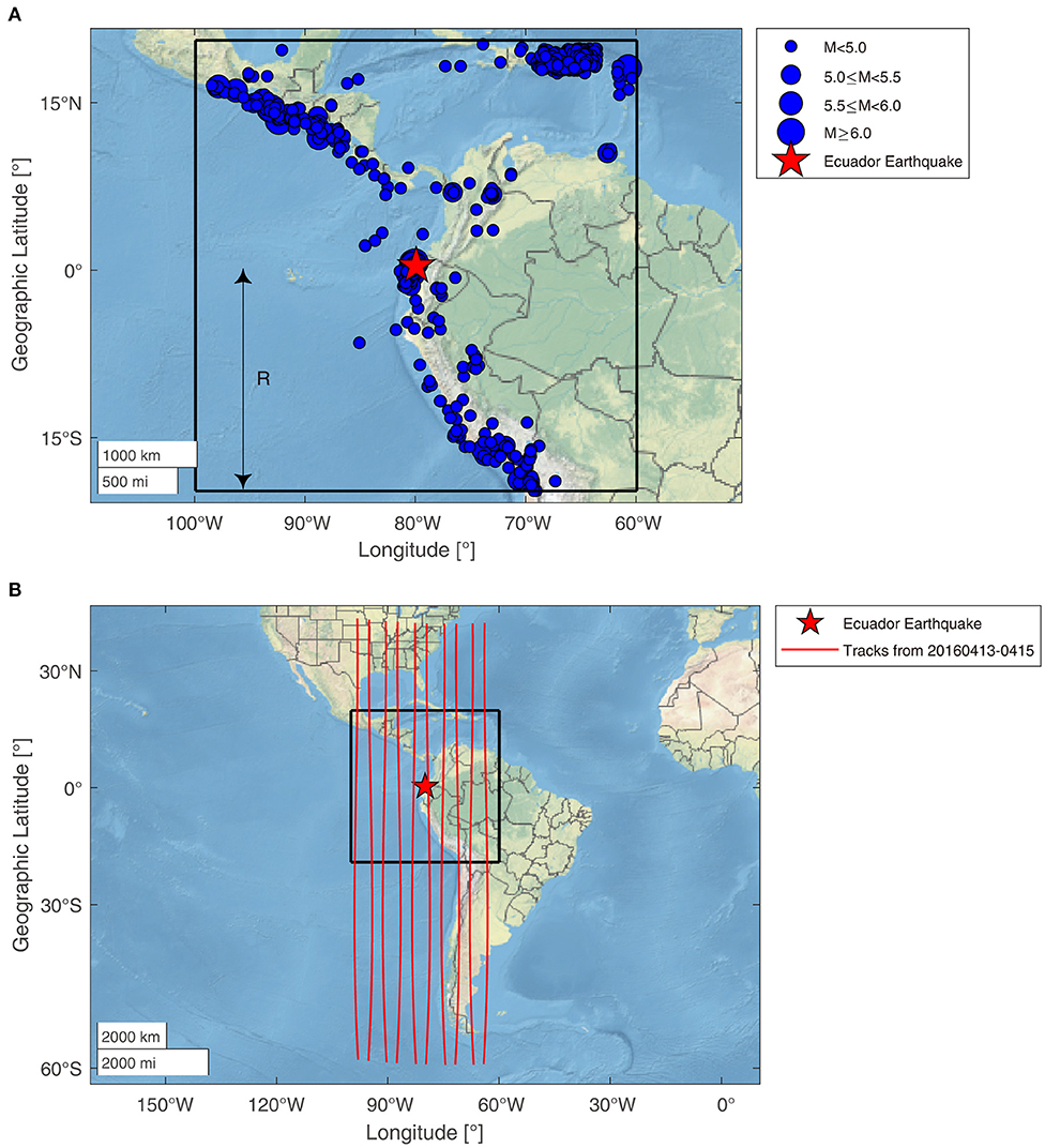
Figure 1. Geographical location and earthquake-sensitive area selected for the Ecuador earthquake. The geographical distribution of the investigated tracks from April 13 to 15, 2016. (A) The epicenter and the earthquake-sensitive area of 2016 Ecuador earthquake. The red star and the black rectangle are the epicenter and the earthquake-sensitive area of the Ecuador earthquake, respectively. The blue dots with black edges mark the earthquakes occurred inside the earthquake-sensitive area from February 16 to May 16, 2016. The half of side length R is the Dobrovolsky's radius strain. (B) The geographical distribution of the investigated tracks from April 13 to 15, 2016. The red lines are investigated tracks.

We studied the tracks that crossed the rectangular region, with R = 2259.4 km (half the side length), which is shown as a black rectangle in Figure 1A. The distance, R is the Dobrovolsky radius strain (Dobrovolsky et al., 1979); R = 10^0.43M(M is the magnitude of the earthquakes) estimates the size of the effective precursor manifestation zone of an earthquake. We assumed that the rectangular region was affected by the Ecuador earthquake, and referred to it as the “earthquake-sensitive area,” while the outside area was not influenced by the earthquake. Moreover, the geomagnetic latitudes of the tracks that we investigated ranged from −50° to + 50° (we avoided aurora and polar interferences). Taking April 13–15, 2016, as an example, the tracks of the Swarm A satellites flying over the earthquake-sensitive area are shown in Figure 1B.

Since we expected the influence of earthquakes to occur only near the epicenters, and due to the advantage of NMF to obtain local features from the overall data, we applied NMF to all the observed satellite magnetic field data, and did not delete the data under strong geomagnetic activity. We analyzed 302 effective tracks from February 16 to May 16, 2016.

Swarm Alpha Satellite Magnetic Field Data Decomposition

In this part, we applied NMF to decompose the Y-East component magnetic field data of the Swarm Alpha satellite. First, we preprocessed the magnetic field data. For each track, the predicted value from the CHAOS-6 geomagnetic field model was subtracted from the magnetic field measurement to remove the core and the static crustal magnetic fields (Finlay et al., 2016). Then, we calculated the first difference of the residuals, along the tracks. The preprocessed magnetic field data for one track data is represented by the vector X as reported in Equation (7).

$\begin{array}{ll}X=\left[x_1{,x}_2,\dots {,x}_{L-1}\right]& (7)\end{array}$

where, L is the number of samples along the track.

After preprocessing, we performed STFT to X, setting the window length to be equal to 64 and the step length to be equal to 16 (with 1 Hz sampling rate of the data, the spatial resolution would be about 122 km). Then the STFT magnitude spectrum V was decomposed by NMF to three basis vectors, namely W_*1, W_*2, and W_*3, and their corresponding weights, H_1*, H_2*, and H_3*, as shown in Equation 8, with the number of basis vector, r = 3. For convenience, we refer below the three basis vectors as W1, W2, and W3, and the three corresponding weights as H1, H2, and H3. In addition, we set the times of the iterative update threshold, N_iter= 1000, the balance parameter α = 0.001 in Equations (2) and (4), and the error factor, ε = 0.0001 in Equation (5).

$\begin{array}{ll}V\approx \left[W_{*1}{W}_{*2}{W}_{*3}\right]\left[\begin{array}{c}{H}_{1^{*}}\\ H_{2^{*}}\\ H_{3^{*}}\\ \end{array}\right]& (8)\end{array}$

The magnitude spectrum, V describes the amplitude–frequency characteristics at different locations along the track. The W1, W2, and W3 describe the basis features (vertical structure) of V. H1, H2, and H3 describe the weight coefficients of the three basis features over location and could show where the features W1, W2, and W3 appeared along the track. If there exists a basis feature, Wx (x = 1, 2, or 3), the high value of the corresponding weight Hx concentrates inside the earthquake-sensitive area; this feature reflects the local feature of the area and it is possibly associated with the Ecuador earthquake. We regarded it as a kind of anomaly inside the earthquake-sensitive area.

Taking one track on April 9, 2016 as an example, the NMF decomposition results of the Y-East component magnetic field data for this track is shown in Figure 2. The preprocessed magnetic field data of the track is shown in Figure 2A. The STFT magnitude spectrum V of the data is shown in Figure 2B. The three basis vectors, W1, W2, and W3 are shown in Figure 2C. The three weight components, H1, H2, and H3 are shown in Figure 2D.

FIGURE 2

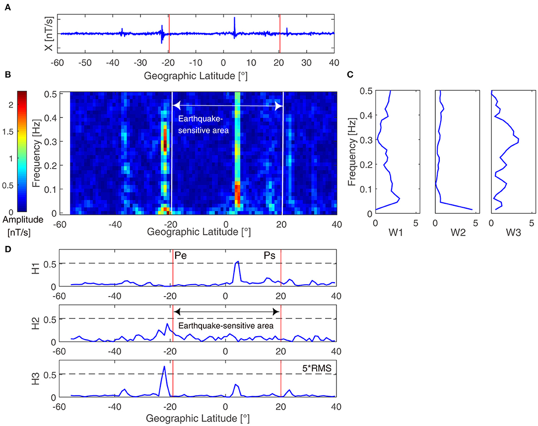
Figure 2. The NMF decomposition results of the Y-East component magnetic field data of a track on April 9, 2016. (A) The preprocessed Y-East component magnetic field data of this track. The red lines show the edges of the earthquake-sensitive area. (B) The STFT magnitude spectrum V of this track. The white lines show the edges of the earthquake-sensitive area. (C) The three basis vectors W1, W2, and W3 of magnitude spectrum V decomposed by NMF. (D) The three weight components H1, H2, and H3 corresponding to the basis vectors. The points between P_s and P_e are inside the earthquake-sensitive area. The red lines show the edges of the earthquake-sensitive area. The black horizontal dotted lines show the 5 times RMS of the components, H1, H2, and H3, respectively.

As shown in Figures 2A,B, before applying NMF, the features of the preprocessed data occurred inside and outside the earthquake-sensitive area. After decomposition, in Figures 2C,D, for feature W1, the corresponding weight, H1 has high values inside the earthquake-sensitive area at ~5° N latitude [with the highest value of 0.5560 which is over 5^*RMS (Root Mean Square) of H1], and it has low values outside the area. For feature W2, the corresponding weight, H2 has slightly high values outside the earthquake-sensitive area (with the highest value of 0.4015, which is 0.78 of 5^*RMS of H2). For feature W3, the corresponding weight, H3 has a very high value at approximately 22° S latitude outside the earthquake-sensitive area (with the highest value of 0.6831, which is over the 5^*RMS of H3) and slightly higher weights inside the area (with the highest value of 0.28244, which exceeds the 5^*RMS of H3 by half of the same value). From these decomposition results, for the example track, the high values of weight, H1 is concentrated inside the earthquake-sensitive area. Thus, the basis feature of W1 reflects the local feature of this area and is possibly associated with the Ecuador earthquake. The high value of H1 is an anomaly inside the earthquake-sensitive area.

The basis vectors describe features and their corresponding weights describe where these features are located along the track. We utilized the weight H components to detect whether anomalies existed inside the earthquake-sensitive area, which are possibly related to earthquakes. The higher the concentration of the H components concentrated inside the earthquake-sensitive area, the more likely this component would have anomalies inside the earthquake-sensitive area. We evaluated the concentration of energy and entropy inside the earthquake-sensitive area for three H components of all the studied tracks, by the energy-entropy ratio. The energy-entropy ratio shows the energy and entropy of the earthquake-sensitive area over those of the whole track, as shown in Equation (9).

$\begin{array}{ll}{\gamma }_n=\frac{\frac{{\displaystyle {\sum }_{j=P_s}^{P_e}}{H{n}_j}^2}{{\displaystyle {\sum }_{j=1}^N}{H{n}_j}^2}+\frac{Z_{inXsn}}{Z_{sXsn}}}{2},(n=1,2,3)& (9)\end{array}$

where, the points between P_s and P_eare located inside the earthquake-sensitive area, as shown in Figure 2D. Xsn is the time-domain reconstruction signal for the Hn component. Z_sXsn is the Shannon entropy (Shannon, 2001) of the whole track for Xsn, and Z_inXsn is the entropy inside the earthquake-sensitive area for Xsn.

The average and standard deviation of the largest energy-entropy ratio, the second largest energy-entropy ratio, and the smallest energy-entropy ratio for the three decomposed H components of all the studied tracks are 0.571±0.106, 0.456 ±0.114, and 0.340 ±0.103, respectively. The largest average value is 25.22% higher than the second largest average value, and 67.94% higher than the smallest average value. From this statistical result, we could see that there existed an H component among the three decomposed H components, whose energy and entropy is much more concentrated inside the earthquake-sensitive area than in the other two H components. Therefore, this H component is more likely to have anomalies inside the earthquake-sensitive area, which is possibly related to the Ecuador earthquake. We refer to this component as Hs1 (the H component with the largest energy-entropy ratio), and the remaining two H components as Hs2 and Hs3, by the descending order of their energy-entropy ratio.

Definition of Anomalous Tracks

Here, we defined the anomalous tracks for the H components. We calculated the RMS of the Hsn (n = 1, 2, or 3) component and set the threshold, K^*RMS (K = 5). The values that exceeded the threshold are the anomalies of this Hsn component, and a track with one or more anomalies is an anomalous track for this Hsn component. The track is an inside anomalous track for this Hsn component, if one or more anomalies occurred inside the earthquake-sensitive area. The track is an outside anomalous track for this Hsn component, if one or more anomalies occurred outside the earthquake-sensitive area. For example, the track in Figure 2 is an inside anomalous track for Hs1 component, but an outside anomalous track for Hs3 component.

Results

In this part, we calculated the cumulative number of inside anomalous tracks for Hs1 component, from 60 days before the earthquake to 30 days after the earthquake, to study the Ecuador earthquake. In addition, the cumulative number of inside anomalous tracks for Hs2 and Hs3 components and that of the outside anomalous tracks for the three H components were also computed for comparison. Finally, we obtained six cumulative results over time, which are presented in Figure 3. The three inside cumulative results are shown in Figure 3A, and the three outside cumulative results are shown in Figure 3B.

FIGURE 3

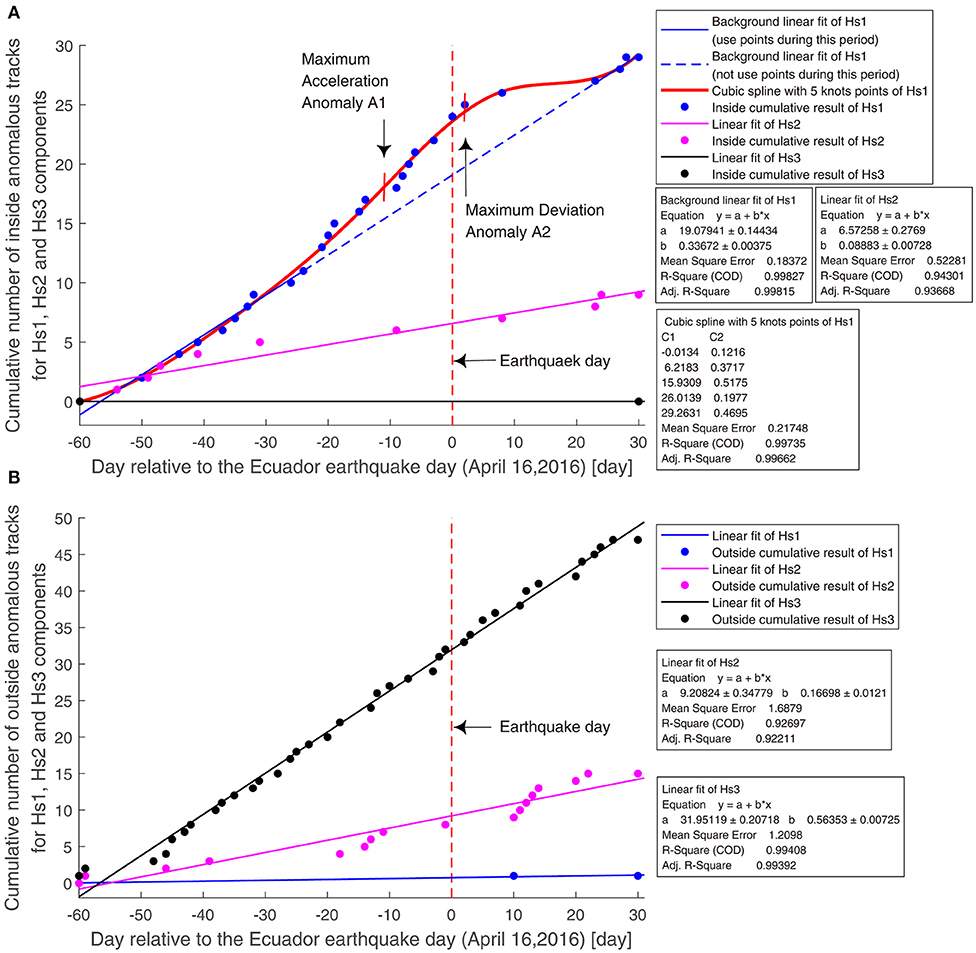
Figure 3. The cumulative number of inside anomalous tracks and those of outside anomalous tracks for components Hs1, Hs2, and Hs3, from 60 days before to 30 days after the earthquake. (A) The cumulative number of inside anomalous tracks for components Hs1, Hs2 and Hs3. The red curve is the cubic spline with 5-knots points using all points. The solid line indicates that we use the points during this period to do the linear fit. The dashed line indicates that we do not use the points during this period to do the linear fit. The day of the earthquake is represented as a red vertical dotted line. (B) The cumulative number of outside anomalous tracks for components, Hs1, Hs2, and Hs3. The day of the earthquake is represented as a red vertical dotted line.

Moreover, if there are nx anomalous tracks on the t^th day, the cumulative sequence Nx(t) is increased by nx on the previous day. For the cumulative results without any value on the first day (day −60), we made 0 as the value of the first day (day −60). For the cumulative results without any value on the last day of the cumulative (day +30), we made the last value of the result as the value of this day (day +30). Thus, all the cumulative results had values on the first day and last day during the cumulative range. In this way, all the cumulative results had exactly the same time range, and all the results show the variation of the entire investigated time range.

For the inside cumulative result of Hs1 component, we performed sigmoid fit, 3-degree polynomial fit, 6-degree polynomial fit, cubic spline with 2-knot points, and cubic spline with 5- knot points (D'Errico, 2021), using all of the blue points. The two cubic spline fits are constrained to be monotonical. We compared the mean squared error, adjusted the coefficient of determination and akaike information criterion, and found that the cubic spline with 5-knot points has the best fitting effect. Thus, for the inside cumulative result of Hs1 component, we performed a cubic spline with 5-knot points using all of the points, as shown in the red curve in Figure 3A. Based on this fit, we selected the points from day −60 to day −24 and from day +23 to day +30, and performed a linear fit to show the anomaly part of the cumulative result and we referred to it as background linear fit of the Hs1 component.

In Figure 3A, the inside cumulative result of Hs1 component shows a clear acceleration before the earthquake, deviating from the previous linear growth, and then recovers after the event. Compared to this result, the inside cumulative result of Hs2 exhibits approximately linear growth, and the Hs3 component does not have an inside anomalous track, as shown in Figure 3A.

As shown in Figure 3B, Hs1 component has only one outside anomalous track. The outside cumulative result of the Hs2 component presents roughly a linear growth. There are two clear increase groups in the cumulative result. We checked the Dst, a_p, and AE indices of the anomalous tracks for these two groups. The group from-14 days to −11 days has three anomalous tracks, two of them with |Dst| > 20 nT and a_p > 10 nT. The group from +10 days to +14 days has five anomalous tracks; the tracks in day +11, day +12, and day +14 present values of the AE index higher than 100 nT, 80 nT, and 300 nT, respectively. Moreover, the AE index is 299 nT 2 h before the anomalous track in day +11 and 3 h before the anomalous track in day +12. From these results, we infer that the anomalous tracks of these two groups are likely to be affected by the geomagnetic activity. The outside cumulative result of Hs3 component shows a quasi-linear trend.

Moreover, on comparing the cumulative number of inside cumulative results with those outside for the three H components, we found that almost all anomalies of Hs1 component occur inside the earthquake-sensitive area. However, for the Hs2 component, some anomalies are located inside the earthquake-sensitive area, some anomalies are located outside this area, and all anomalies of Hs3 component are outside the earthquake-sensitive area. From these results, we found that the inside cumulative result of Hs1 component is more likely to reflect the anomalies of the Ecuador earthquake.

Then, we further analyzed the inside result of the Hs1 component. From Figure 3A, until 20 days before the main shock, the cumulative number of Hs1 has exhibited linear growth and then begins to show accelerated growth. The increased speed reaches its maximum 11 days before the main shock, which is shown as the maximum acceleration anomaly, A1 in Figure 3A. Meanwhile, the cumulative number deviates from the previous linear growth, and the deviation extent reaches its highest in 2 days after the Ecuador earthquake, which is shown as the maximum deviation anomaly, A2 in Figure 3A. Eight days after the main shock, the cumulative number stops increasing temporarily, which is consistent with the deceleration time of the aftershock cumulative seismicity for the northern and southern patches (Agurto-Detzel et al., 2019). Thus, we speculated that the gap between +8 days to +22 days is possibly affected by the decrease of the seismic activity. Then, 23 days after the main shock, the cumulative number recovers to its linear growth. The abnormal phenomenon of the inside cumulative result for Hs1 component that the cumulative number accelerated before the earthquake and recovered after it is consistent with the studies of De Santis et al. (2017, 2019c). These studies indicated that the cumulative number of anomalies for a critical system would accelerate when approaching its critical time and recover after a large event (De Santis et al., 2017, 2019c), that is, the 7.8 Mw earthquake.

We also found that the accelerated cumulative anomaly of Hs1 component is similar to the results of the other two studies on the Ecuador earthquake, which also used the magnetic field data of the Swarm satellites but excluded the influences of the geomagnetic activity. The maximum acceleration anomaly, A1 in Figure 3A corresponds to a study by Akhoondzadeh et al. (2018). Their study shows that the cumulative number of anomalous tracks accelerates ~9 days before the Ecuador earthquake, when the magnetic field data collected under quiet geomagnetic conditions are considered. The maximum deviation anomaly, A2 in Figure 3A is consistent with the study of Zhu et al. (2019). Their study indicated that the increased speed of the cumulative number of anomalous tracks reaches its maximum around the time of the Ecuador earthquake, after using principal component analysis to remove the component affected by geomagnetic activity.

In addition, we performed some confutation analysis to prove that the accelerated cumulative anomaly is possibly related to the Ecuador earthquake rather than caused by other disturbances.

Confutation Analysis

Geomagnetic Activity Influence Study

To study whether the accelerated cumulative anomaly of Hs1 component is affected by geomagnetic activity, we performed two types of research. First, we analyzed the correlation between the time-domain reconstruction signal of Hs1 component and the geomagnetic index and compared the results with those of the original time domain signal and the other two H components.

For each investigated track (from 30 days before the earthquake to 30 days after the earthquake), we computed the median value of the time-domain signal X before the NMF decomposition and those of the time-domain reconstruction signal for the H components, Xs1, Xs2, Xs3 and Xs2 + Xs3. We compared the variation of the median value for the signals with their corresponding a_p index [from the International Service of Geomagnetic Indices (ISGI)], as shown in Figure 4.

FIGURE 4

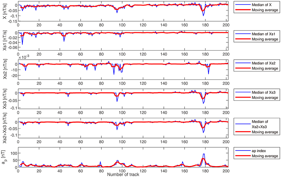
Figure 4. The median value of the X, Xs1, Xs2, Xs3, and Xs2 + Xs3 from 30 days before to 30 days after the earthquake, and their corresponding a_pindex. The X is the time domain signal before the NMF decomposition. The Xs1, Xs2, Xs3, and Xs2 +Xs3 are the time-domain reconstruction signal of H components. The red curves are the moving averages of the signals.

In Figure 4, Xs1 is not significantly correlated to the a_p index, but the X, Xs3 and Xs2 + Xs3 seem to be adequately correlated with the geomagnetic a_p index. Then, we calculated the correlation coefficient between the a_p index and X, Xs1, Xs2, Xs3, and Xs2 + Xs3, where the results show the values, a −0.76, −0.20, −0.40, −0.82, and −0.84, respectively. These results reflect that the time-domain signals, X, Xs3, and Xs2, + Xs3 have strong correlations with the a_p index; the absolute values of these correlation coefficients are over 0.8. In contrast, the correlation coefficient between Xs1 and the a_p index is very low; the absolute value of the correlation coefficient is 0.20. Thus, after the NMF decomposition, the signal influenced by the geomagnetic activity seems to be included in the Xs2 and Xs3 components. However, the Xs1 component is not likely to relate to the geomagnetic activity.

Second, we examined the influence of the geomagnetic activity on the anomalous tracks of Hs1 component, and compared the results with those of the other two components. We set the Dst index (from ISGI) classification standard and divided the spatial conditions into four levels, from L0 toL3. Then, we calculated the numbers and percentages of anomalous tracks for Hs1, Hs2, and Hs3 components, before the earthquake, at different Dst levels, as shown in Table 1.

TABLE 1

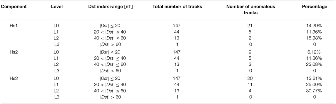
Table 1. The numbers and percentages of anomalous tracks for Hs1, Hs2, and Hs3 components at different Dst levels before the Ecuador earthquake.

From Table 1, with the increase of the Dst level, the percentage of anomalous tracks for the Hs1 component shows a slight fluctuation; it first decreases by 20% and then increases by 35%. The percentage of anomalous tracks for the Hs2 and Hs3 components continuously increase with stronger geomagnetic activity. The percentage of anomalous tracks for Hs2 increases by 85% and then increases by 103%. At the L0 level, the percentage of anomalous tracks for the Hs3 is similar to Hs1, but at the L₂ and L₁ levels, the results of Hs3 are approximately twice as large as those of Hs1. Therefore, the anomalous tracks of Hs2 and Hs3 components are likely to be influenced by the geomagnetic activity. However, the anomalous tracks of Hs1 component are almost not affected by the geomagnetic activity.

From these two studies, we come to know that the accelerated cumulative anomaly of Hs1 component is hardly influenced by the geomagnetic activity.

We also assess the solar activity index, namely the F10.7 index within the study time range. Although the solar activity index near the earthquake is high [max: 107 solar flux unit (sfu)], no sudden change is evident. In addition, a previous study showed that the solar radio flux parameter probably did not affect the seismo-ionospheric anomalies detected around the date of Ecuador earthquake (Akhoondzadeh et al., 2018). Therefore, we did not consider the influence of the solar activity index, F10.7 on the ionosphere magnetic anomalies.

Plasma Bubbles Influence Study

The ionospheric magnetic field data might be affected by small-scale ionospheric irregularities, namely plasma bubbles. To explore whether the accelerated cumulative anomaly of Hs1 component is affected by plasma bubbles, we checked the Bubble index and the Bubble probability of the anomalous tracks (Park et al., 2013).

Both the Bubble index and the Bubble probability of the points inside the earthquake-sensitive area of the inside anomalous tracks for Hs1 component, from day−14 to day +2, at the critical accelerated phase are 0, which means that the data are not affected by the plasma bubbles. So, we can speculate that the accelerated cumulative anomaly of Hs1 component is not probably caused by the plasma bubble.

Random Earthquake Study and Low-Seismicity Period Study

In this section, we performed a random earthquake study proposed by Parrot (2011) and low-seismicity period study to analyze the relationship between the Ecuador earthquake and the accelerated cumulative anomaly of the magnetic field data.

We randomly selected four pseudo earthquake epicenters around the world, which cover different latitude positions (excluding high latitudes), and studied them with the same time duration and the same size of earthquake-sensitive area as those of the Ecuador earthquake, without earthquakes over 5.5, as shown in Table 2 and Figure 5. In particular, we noted that the latitude of the Random 1 epicenter is similar to that of the Ecuador earthquake epicenter and the Random 2 epicenter is in a region that sometime has active ionospheric irregularities (Yizengaw and Groves, 2018). The LT of the four random pseudo earthquakes is almost the same as that of the Ecuador earthquake.

TABLE 2

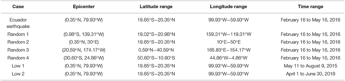
Table 2. The locations, earthquake-sensitive areas, and study time ranges of Ecuador earthquake, four random pseudo earthquakes, and two low-seismicity period cases.

FIGURE 5

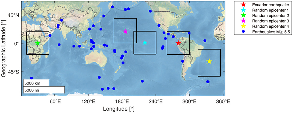
Figure 5. The geographical locations and earthquake-sensitive areas of the Ecuador earthquake and four random pseudo earthquakes. The black rectangles show the earthquake-sensitive areas of the Ecuador earthquake and four random pseudo earthquakes. The blue dots show the earthquakes with magnitude ≥5.5 worldwide from February 16 to May 16, 2016.

We also studied two low-seismicity periods with the same location and earthquake-sensitive area as those of the Ecuador earthquake; no earthquake with a magnitude over 5.8 occurred in these two periods, as shown in Table 2. Although the LT of the data for the two cases are not exactly same with those for the Ecuador earthquake, they cover the LT (sweeps from 21 to 20 LT for nighttime tracks and from 9 to 8 LT for daytime tracks) at the increased phase of the cumulative results.

Likewise, we calculated the cumulative number of the inside anomalous tracks of Hs1 component for the four random pseudo earthquakes and two low-seismicity periods, and then compared them with the cumulative results of the Ecuador earthquake, as shown in Figures 6, 7.

FIGURE 6

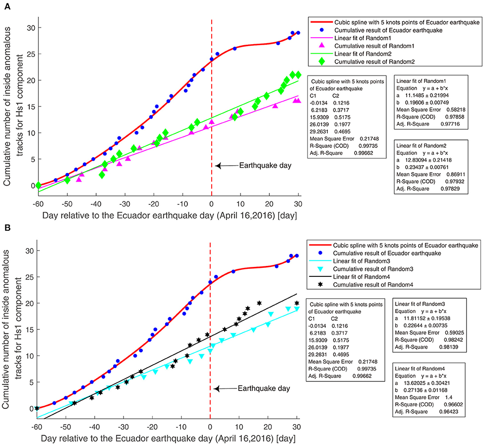
Figure 6. The cumulative number of inside anomalous tracks of Hs1 component for the Ecuador earthquake and the four random pseudo earthquakes. (A) The cumulative results for two low latitude random pseudo earthquakes, Random 1, Random 2, and the Ecuador earthquake. The day of the earthquake is represented as a red vertical dotted line. (B) The cumulative results for two middle latitude random pseudo earthquakes, Random 3, Random 4, and the Ecuador earthquake. The day of the earthquake is represented as a red vertical dotted line.

FIGURE 7

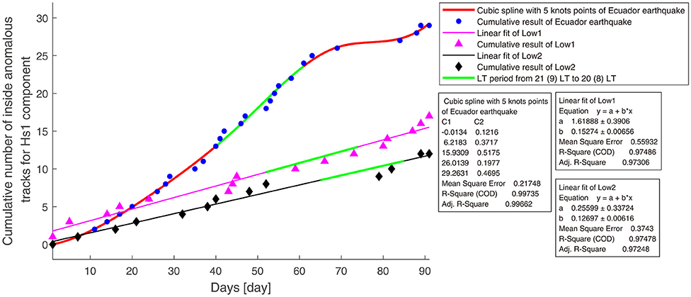
Figure 7. The cumulative number of inside anomalous tracks of Hs1 component for the Ecuador earthquake and two low-seismicity period cases. The green curves show the LT period from 21 (9) to 20 (8) LT for the three cumulative results.

In Figures 6, 7, the cumulative number of the inside anomalous tracks for four random pseudo earthquakes and two low-seismicity period cases show approximately linear growth. To avoid the influence of LT, we checked the cumulative results of Low 1 and Low 2 from 21 (9) to 20 (8) LT, as shown by the green curves in Figure 7, and we found that they did not show accelerated increase. Thus, in non-earthquake regions or during non-earthquake periods, the cumulative results exhibited linear increase trend. The results are consistent with the “typical random process,” proposed by De Santis et al. (2017); for a random process, the accumulated value is expected to show a statistically linear increase. However, for the actual Ecuador earthquake, as the earthquake approaches, the cumulative number of anomalous tracks accelerates growth and then recovers after the event, confirming that this trend seems to be related to the seismic event.

Moreover, from Figure 6 before the day of the earthquake, the average number of anomalous tracks for the four random earthquakes is ~10, while the number of anomalous tracks of the real Ecuador earthquake is ~25. This result shows that the number of anomalies for non-earthquake region cases is less than that of the real earthquake, which possibly supports the earthquake source of at least a subset of the anomalies (15 during the 2 months before the Ecuador earthquake), which is also consistent with the study of Parrot (2011).

These results further verify that the accelerated cumulative anomaly of Hs1 component of the ionosphere magnetic field is not obtained by simple chance or influenced by the study time period, geographical location, and LT, and it is possibly associated with the Ecuador earthquake.

Cumulative Benioff Strain S Study

In this section, we studied the correlation between the accelerated cumulative anomaly of the ionosphere magnetic field data and the lithosphere activities. Considering the cumulative effect of a series of N earthquakes before a large earthquake, we calculated the cumulative Benioff strain S (Benioff, 1949; De Santis et al., 2019a), which could estimate the strain-rebound increment by the earthquake energy, to study the lithosphere activity before the Ecuador earthquake, and compared it with the cumulative result of Hs1 component for the ionosphere magnetic field data.

Because of the limitations in the detection capability of the seismograph network, some weak earthquakes are not recorded. We used the maximum curvature technique (Xie et al., 2019) to estimate the smallest magnitude Mc that could be completely detected in the seismic-relevant area (with half large size of the earthquake-sensitive area of the Ecuador earthquake). The estimated complete magnitude is Mc = 4.3 by the seismic events (from USGS) in 2016. Then we selected the seismic events with magnitudes ≥4.3 and hypocentral depths ≤50 km, from February 16, 2016 until the moment of the Ecuador earthquake, in the seismic-relevant area to calculate the cumulative Benioff strain S.

For each selected seismic event, we calculated the released energy as explained in Equation (10) (Han et al., 2014).

$\begin{array}{ll}{E}_i=10^{4.8+1.5M_i}& (10)\end{array}$

where, Mi is the magnitude of the ith earthquake. Then we computed the cumulative Benioff strain S as explained in Equation (11) (Marchetti et al., 2019c).

$\begin{array}{ll}S={\displaystyle \sum _{i=1}^{nc}}\sqrt{E_i}& (11)\end{array}$

where, nc is the total number of the earthquakes.

The cumulative Benioff strain S around the epicenter of the Ecuador earthquake and the cumulative number of the inside anomalous tracks of Hs1 component for ionospheric magnetic field data are shown in Figure 8.

FIGURE 8

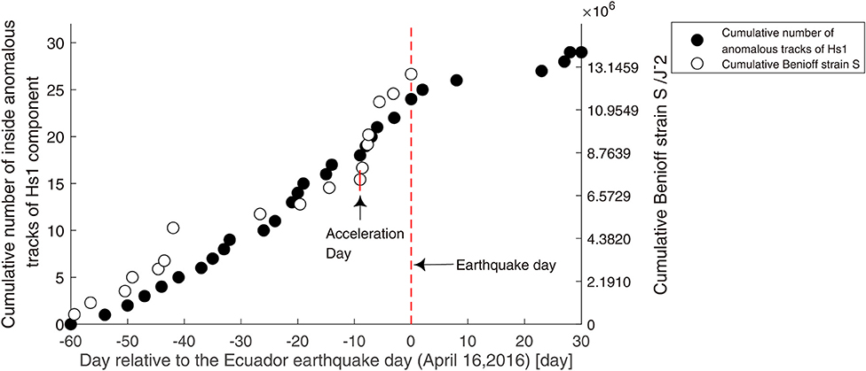
Figure 8. The cumulative Benioff strain S around the Ecuador earthquake epicenter and the cumulative number of inside anomalous tracks of Hs1 component for the magnetic field data, from February 16, 2016, to May 16, 2016. The day of the earthquake is represented as a red vertical dotted line.

In Figure 8, until 8 days before the main shock, the cumulative Benioff strain S shows an approximate linear increase. After this day, the cumulative result shows a trend of accelerated growth and it continues until the moment of occurrence before the Ecuador earthquake. The clustering of earthquakes before a large earthquake might be a result of several physical mechanisms operating in the seismogenic crust (Shcherbakov et al., 2019). Therefore, this acceleration phenomenon may correspond to the energy release before the Ecuador earthquake and may be connected to the lithosphere activities before the earthquake, that is, the seismic activation of the fault system (Marchetti et al., 2019c).

Comparing the cumulative Benioff strain S and the cumulative results of Hs1 component of the ionosphere magnetic field data, we found that they have similar accelerate growth trend before the earthquake. And, as the earthquake approached, the anomaly phenomena in both the ionosphere and lithosphere became more and more obvious. Meanwhile, the acceleration day (8 days before the earthquake) of the cumulative Benioff strain S is near the day (11 days before the earthquake) when the increased speed of the cumulative number of the magnetic field data reached its maximum. This consistency indicates that the accelerated cumulative anomaly of Hs1 component for the ionosphere magnetic field data are possibly associated with the lithosphere activities, which are related to the Ecuador earthquake.

The correspondence between the accelerated cumulative anomaly of the ionosphere magnetic field data and the lithosphere activities is consistent with the study on the Nepal earthquake by De Santis et al. (2017). This study indicates that the cumulative number of ionosphere magnetic anomalies and those of M4+ earthquakes have similar trends before and after the earthquake. By De Santis, this similar behavior between them supports the LAIC and the hypothesis that “the noticed magnetic anomalies in Swarm data are mostly of internal origin, due to a LAI coupling.”

According to LAIC models, the anomalies, which occurred in different layers before strong earthquakes, could be explained as a synergy between the lithosphere, atmosphere (included the Earth's surface), and ionosphere processes and anomalous variations which are usually named as medium/short-term earthquake precursors. From the LAIC model, before the earthquake, fault activation releases some positive charged holes (Freund, 2011) or leads to gas migration including radon emanation (Pulinets and Ouzounov, 2011). Then the release of radon induces the ionization of the atmosphere. Formation of large ion clusters led to variations in the atmospheric electricity which is the main source of ionospheric anomalies over seismically active areas including the electromagnetic anomaly before the earthquake. Other coupling mechanisms have also been hypnotized; for example, a complete electric coupling induced by a change in the ground resistivity due to the variation of the strain on the fault (Kuo et al., 2014), or even a surface warming could produce an acoustic gravity wave before the occurrence of the earthquake (Hayakawa, 2011).

This correspondence between the anomalous behavior in the ionosphere and that in the lithosphere is consistent with the synergy among the processes of the different layers, and their anomalies are explained by one of the LAIC models. Therefore, our result supports the LAIC effects and we suggest that the Ecuador earthquake possibly involved a physical coupling between the lithosphere and the ionosphere in its preparation phase, and the accelerated cumulative anomaly of Hs1 component for the ionosphere magnetic field data is likely to originate in the lithosphere.

Investigation of Anomalies During the Accelerated Increase Phase

We investigated the anomalies extracted during the accelerated increase phase, from 26 days before the earthquake to the day of the earthquake (the anomalies in these days are more possibly related to the earthquake).

We checked the extracted anomalies one by one and found that the anomaly at track 5 on April 2, 2016, 14 days before the earthquake, is the closest anomaly to the epicenter of the Ecuador earthquake (<500 km away from the epicenter). The preprocessed East component of magnetic field data X for this anomalous track, the time-domain reconstruction signals, Xs1, Xs2, and Xs3 of the three decomposition components of this track, the feature Ws1, the weight, Hs1 and the location of this anomaly are shown in Figure 9. From Figure 9, it is clear that in Xs1, the anomaly lasted from −7° latitude to +7° latitude and the maximum value of this anomaly is almost at the same latitude of the epicenter. According to Ws1, the frequency with the highest amplitude of this anomaly is around 0.36 Hz. According to Hs1, the weight of this anomaly is surely concentrated inside the earthquake-sensitive area. Compared with Xs1, the original data X has two obvious anomalies. The northern one centered about at 0° latitude is found also in Xs1, while a double pattern is found in Xs2 and Xs3. Although these two anomalies in X are nearer and symmetrical to the geomagnetic equator (around −10° geographic latitude), the LT is 21 o'clock, they are not directly to be affected by the sunset. Moreover, the NFM technique underlines that the northern anomaly is different from the standard double pattern, which could be a residual of the daily interaction between the Sun and the ionosphere. From these results, the anomaly of Xs1 is more likely related to the earthquake.

FIGURE 9

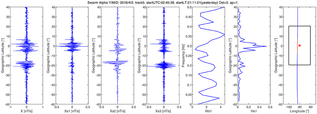
Figure 9. Analysis of the anomaly closer to the epicenter of the Ecuador earthquake which occurred in the anomalous track on April 2, 2016. X represents the preprocessed East component of magnetic field data for this track. Xs1, Xs2, and Xs3 are the time-domain reconstruction signals of three decomposition component of this track. The Ws1 and Hs1 are, respectively, the feature and weight of this anomaly. The red star represents the epicenter of the Ecuador earthquake and the black square represents the earthquake-sensitive area of the earthquake. The blue line represents the flight path of this track. The short red line shows the location of this anomaly.

In addition, we analyzed the relationship between the amplitude of anomalies and their distance from the epicenters, from 26 days before the earthquake to the day of the earthquake. The smallest distance from the epicenter is 465 km and the largest distance from the epicenter is 2,792 km. We divided the anomalies into three groups, according to their distance from the epicenter. For each group, we calculated the average energy of the anomalies. The relationship between the average energy of the anomalies and their distances from the epicenter is shown in Figure 10A. From Figure 10A, we can see that as the location of the anomaly is farther from the epicenter of the earthquake, the average energy of the anomaly decreased. This result is consistent with one of the standards for excellent earthquake precursors proposed by the International Association of Seismology and Physics of Earth's Interior (IASPEI) in 1991 and 1997 (Wyss, 1991, 1997; Wyss and Booth, 1997). This standard observes that “the amplitude of the observed anomaly should bear a relation to the distance from the eventual mainshock,” and it is also affirmed by Rikitake and Yamazaki (1985).

FIGURE 10

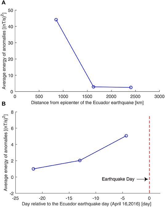
Figure 10. The investigations of the average energy of the anomalies. (A)The relationship between the average energy of the anomalies and the distance from the epicenter of the anomalies. (B) The relationship between the average energy of the anomalies and the occurrence time of anomalies. The anomalies were extracted from 26 days before the earthquake to the day of the earthquake.

The relationship between the amplitude and the time of occurrence of the anomalies was also investigated. The anomalies were divided into three groups, according to their time of occurrence. The average energy of the anomalies for each group was computed. The relationship between the average energy of the anomalies and their occurrence time is shown in Figure 10B. According to Figure 10B, at the advent of earthquake, the average energy of the anomalies increased. This result is reasonable, since generally with the advent of the earthquake, the anomalies should be stronger.

These two analyses further prove that the anomalies we extracted at the accelerated increase phase before the earthquake are likely to be related to the earthquake.

Conclusions

In this paper, we used the NMF to analyze the magnetic field data of Swarm Alpha satellite and explored the 2016 Mw 7.8 Ecuador earthquake, including all the observation data, regardless of the strength of the geomagnetic activity. After decomposition, we obtained three H components, and found that almost all the anomalies of one of the H components, that is the Hs1 component, occurred inside the earthquake-sensitive area, and the inside cumulative result of this component showed a clear acceleration before the Ecuador earthquake and recovered after it, which obeys the power-law behavior of a critical system (De Santis et al., 2017). By different analyses, we excluded the influence of the geomagnetic activity and the plasma bubbles on the accelerated cumulative anomaly, and proved that this anomaly was not obtained by simple chance. Moreover, we found that the accelerated cumulative anomaly for the ionosphere magnetic field data was possibly associated with the lithosphere activities before the Ecuador earthquake, which also corresponds to the LAIC effect. By investigating the anomalies, we further found that as the location of the anomaly is farther from the epicenter of the earthquake, the average energy of the anomaly decreased, and with the advent of the earthquake, the average energy of the anomalies increased. Thus, the anomalies that we extracted are possibly related to the Ecuador earthquake.

These abovementioned results show that the NMF method has the capacity to detect the local feature of the earthquake-sensitive area. For the Ecuador earthquake, based on NMF decomposition, by using all the observed magnetic field data without considering the geomagnetic activity, we obtained a weight component, whose cumulative result has an accelerated anomaly that is possibly related to the earthquake and not affected by the geomagnetic activity. This type of method could introduce a new perspective and analyze as much observation data as possible to study the earthquakes.

We suggest that our paper promotes the development from the search of anomalies that are likely to be related to earthquakes at the quiet geomagnetic conditions (which is still a difficult task) to the search of the anomalies that are likely to be related to earthquakes without considering the geomagnetic activity. We propose to address this problem with the use of NMF, but we do not exclude other methods that can more efficiently achieve the same goal.

We remind that the objective of these present analyses is not a retrospective prediction of an earthquake, but to emphasize that by NMF, we can use more data to analyze earthquakes. We would expect that using the satellite magnetic field data without considering the geomagnetic condition might be a better and more comprehensive method to understand earthquakes than using the data at quiet geomagnetic conditions alone.

In addition, further study should analyze the regular patterns among the local feature of the earthquake-sensitive area for different tracks. More case studies should be undertaken especially the investigation of other large earthquakes will be an important matter for future work.

Data Availability Statement

Publicly available datasets were analyzed in this study. This data can be found here: Swarm data: https://swarm-diss.eo.esa.int/. The geomagnetic index: http://isgi.unistra.fr/data_download.php. The F10.7: ftp://ftp.ngdc.noaa.gov/STP/swpc_products/daily_reports/space_weather_indices. The seismic data: https://earthquake.usgs.gov/earthquakes/search/.

Author Contributions

KZ conceived and designed the project, guided the writing of the manuscript, and revised the manuscript. MF worked on the data analysis, the interpretation of the data, and wrote the manuscript. XH and KL contributed to data acquisition and revised the manuscript. DM contributed to data interpretation, gave some guiding opinions, and revised the manuscript. ZY, CC, HS, and YC contributed to the data interpretation and revised the manuscript. All authors contributed to the revision of the manuscript, read, and approved the submitted version.

Funding

This research was supported by the National Natural Science Foundation of China under Grant No. 41974084 and the International Cooperation Project of Department of Science and Technology of Jilin Province No. 20200801036GH.

Conflict of Interest

The authors declare that the research was conducted in the absence of any commercial or financial relationships that could be construed as a potential conflict of interest.

Acknowledgments

The authors would like to acknowledge the European Space Agency for the Swarm data, the International Service of Geomagnetic Indices for the Dst index data and a_p index data, the National Oceanic Atmospheric Administration for the F10.7 data, and the United States Geological Survey for the seismic events list data. We are grateful to the College of Instrumentation and Electrical Engineering of Jilin University, the Key Laboratory of Geo-Exploration Instrumentation of the Ministry of Education in Jilin University of China, and the National Institute of Geophysics and Volcanology. We are grateful to Prof. Xuhui Shen (from the Institute of Crustal Dynamics, China Earthquake Administration), Prof. Xiuying Wang (from the Institute of Crustal Dynamics, China Earthquake Administration), and Prof. Angelo De Santis (from the Environment Department of Istituto Nazionale di Geofisica e Vulcanologia, Rome, Italy) for their contribution to this article.

References

Agurto-Detzel, H., Font, Y., Charvis, P., Régnier, M., Rietbrock, A., Ambrois, D., et al. (2019). Ridgesubduction and afterslip control aftershock distribution of the 2016 Mw 7.8 Ecuador earthquake. Earthand Planet. Sci. Lett. 520, 63–76. doi: 10.1016/j.epsl.2019.05.029

CrossRef Full Text | Google Scholar

Akhoondzadeh, M., De Santis, A., Marchetti, D., Piscini, A., and Cianchini, G. (2018). Multi precursorsanalysis associated with the powerful Ecuador (Mw= 7.8) earthquake of 16 April 2016 using Swarmsatellites data in conjunction with other multi-platform satellite and ground data. Adv. Space Res. 61, 248–263. doi: 10.1016/j.asr.2017.07.014

CrossRef Full Text | Google Scholar

Akhoondzadeh, M., De Santis, A., Marchetti, D., Piscini, A., and Jin, S. (2019). Anomalous seismo-laivariations potentially associated with the 2017 Mw=7.3 Sarpol-e Zahab (Iran) earthquake from Swarmsatellites, GPS-TEC and climatological data. Adv. Space Res. 64, 143–158. doi: 10.1016/j.asr.2019.03.020

CrossRef Full Text | Google Scholar

Alken, P. (2016). Observations and modeling of the ionospheric gravity and diamagnetic current systemsfrom CHAMP and Swarm measurements. J. Geophys. Res. Space Phys. 121, 589–601. doi: 10.1002/2015ja022163

CrossRef Full Text | Google Scholar

Benioff, H. (1949). Seismic evidence for the fault origin of oceanic deeps. Bull. Geol. Soc. Am. 60, 1837–1856. doi: 10.1130/0016-7606(1949)60[1837:SEFTFO]2.0.CO;2

CrossRef Full Text | Google Scholar

Bolt, B. A. (1999). Earthquake. NewYork, NY: W. H. Freeman.

Google Scholar

Bouffard, J., Floberghagen, R., and Olsen, N. (2019). The Swarm Satellite Trio Studies Earth and Its Environment. EOS.

Google Scholar

Cichocki, A., Zdunek, R., and Amari, S. (2006). “New algorithm for non-negative matrix factorization inapplication to blind source separation,” in Proceedings of ICASSP'06 (Toulouse: IEEE Press), 621–624.

Google Scholar

De Santis, A., Abbattista, C., Alfonsi, L., Amoruso, L., Campuzano, S. A., Carbone, M., et al. (2019a). Geosystemics view of earthquakes. Entropy 21:412. doi: 10.3390/e21040412

PubMed Abstract | CrossRef Full Text | Google Scholar

De Santis, A., Balasis, G., Pavón-Carrasco, F. J., Cianchini, G., and Mandea, M. (2017). Potential earthquake precursory pattern from space: the 2015 Nepal event as seen by magnetic Swarm satellites. Earth Planet. Sci. Lett. 461, 119–126. doi: 10.1016/j.epsl.2016.12.037

CrossRef Full Text | Google Scholar

De Santis, A., De, F. G., Spogli, L., Perrone, L., Alfonsi, L., Qamili, E., et al. (2015). Geospaceperturbations induced by the earth: the state of the art and future trends. Phys. Chem. Earth 85–86, 17–33. doi: 10.1016/j.pce.2015.05.004

CrossRef Full Text | Google Scholar

De Santis, A., Marchetti, D., Pavon-Carrasco, F. J., Cianchini, G., Perrone, L., Abbattista, C., et al. (2019b). Precursory worldwide signatures of earthquake occurrences on Swarm satellite data. Sci. Rep. 9:20287. doi: 10.1038/s41598-019-56599-1

PubMed Abstract | CrossRef Full Text | Google Scholar

De Santis, A., Marchetti, D., Spogli, L., Cianchini, G., Pavón-Carrasco, F. J., Franceschi, G. D., et al. (2019c). Magnetic field and electron density data analysis from Swarm satellites searching for ionosphericeffects by great earthquakes: 12 case studies from 2014 to 2016. Atmosphere 10:371. doi: 10.3390/atmos10070371

CrossRef Full Text | Google Scholar

D'Errico, J. (2021). SLM - Shape Language Modeling, MATLAB Central File Exchange. Available online at: https://www.mathworks.com/matlabcentral/fileexchange/24443-slm-shape-language-modeling (accessed February 23, 2021).

Dobrovolsky, I. R., Zubkov, S. I., and Myachkin, V. I. (1979). Estimation of the size of earthquakepreparation zones. Pure Appl. Geophys. 117, 1025–1044. doi: 10.1007/BF00876083

CrossRef Full Text | Google Scholar

Finlay, C. C., Olsen, N., Kotsiaros, S., Gillet, N., and Tøffner-Clausen, L. (2016). Recent geomagneticsecular variation from Swarm and ground observatories as estimated in the CHAOS-6 geomagnetic fieldmodel. Earth Planets Space 68:112. doi: 10.1186/s40623-016-0486-1

CrossRef Full Text | Google Scholar

Finlay, C. C., Olsen, N., and Tøffner-Clausen, L. (2015). DTU candidate field models for IGRF-12 and theCHAOS-5 geomagnetic field model. Earth Planets Space 67:114. doi: 10.1186/s40623-015-0274-3

CrossRef Full Text | Google Scholar

Freund, F. (2000). Time-resolved study of charge generation and propagation in igneous rocks. J. Geophys. Res. Solid Earth 105, 11001–11019. doi: 10.1029/1999JB900423

CrossRef Full Text | Google Scholar

Freund, F. (2011). Pre-earthquake signals: underlying physical processes. J. Asian Earth Sci. 41, 383–400. doi: 10.1016/j.jseaes.2010.03.009

CrossRef Full Text | Google Scholar

Friis-Christensen, E., Lühr, H., and Hulot, G. (2006). Swarm: a constellation to study the Earth's magneticfield. Earth Planets Space 58, 351–358. doi: 10.1186/BF03351933

CrossRef Full Text | Google Scholar

Friis-Christensen, E., Lühr, H., Knudsen, D., and Haagmans, R. (2008). Swarm - an earth observationmissioninvestigatinggeospace. Adv. Space Res. 41, 210–216. doi: 10.1016/j.asr.2006.10.008

CrossRef Full Text | Google Scholar

Fu, C., Lee, L., Ouzounov, D., and Jan, J. (2020). Earth's outgoing longwave radiation variability prior to M ≥ 6.0earthquakes in the Taiwan area during 2009-2019. Front. Earth Sci. 8:364. doi: 10.3389/feart.2020.00364

CrossRef Full Text | Google Scholar

Han, P., Hattori, K., Hirokawa, M., Zhuang, J., Chen, C., Febriani, F., et al. (2014). Statistical analysis ofULF seismomagnetic phenomena at Kakioka, Japan, during 2001-2010. J. Geophys. Res. Space Phys. 119, 4998–5011. doi: 10.1002/2014JA019789

CrossRef Full Text | Google Scholar

Hattori, K., and Han, P. (2018). “Statistical analysis and assessment of ultralow frequency magnetic signals inJapan as potential earthquake precursors,” in Pre-earthquake Processes: A Multidisciplinary Approach toEarthquake Prediction Studies, eds D. Ouzounov, S. Pulinets, K. Hattori, and P. Taylor (Hoboken, NJ: John Wiley & Sons), 229–240.

Google Scholar

Hattori, K., Serita, A., Gotoh, K., Yoshino, C., Harada, M., Isezaki, N., et al. (2004). ULF geomagneticanomaly associated with 2000 Izu Islands earthquake swarm, Japan. Phys. Chem. Earth Parts A B C 29, 425–435. doi: 10.1016/j.pce.2003.11.014

CrossRef Full Text | Google Scholar

Hayakawa, M. (2011). On the fluctuation spectra of seismo-electromagnetic phenomena. Nat. Hazards Earth Syst. Sci. 11, 301–308. doi: 10.5194/nhess-11-301-2011

CrossRef Full Text | Google Scholar

Hayakawa, M., and Molchanov, O. A. (2002). Seismo Electromagnetics Lithosphere-Atmosphere-Ionosphere Coupling. Tokyo: TERRA-PUB.

Google Scholar

Ho, Y., Jhuang, H., Lee, L., and Liu, J. (2018). Ionospheric density and velocity anomalies before M ≥ 6.5 earthquakes observed by DEMETER satellite. J. Asian Earth Sci. 166, 210–222. doi: 10.1016/j.jseaes.2018.07.022

CrossRef Full Text | Google Scholar

Kuo, C. L., Lee, L. C., and Huba, J. D. (2014). An improved coupling model for the lithosphere-atmosphere-ionosphere system. J. Geophys. Res.:Space Phys. 119, 3189–3205, doi: 10.1002/2013JA019392

PubMed Abstract | CrossRef Full Text | Google Scholar

Lee, D. D., and Seung, H. S. (1999). Learning the parts of objects by non-negative matrix factorization. Nature 401, 788–791.

PubMed Abstract | Google Scholar

Lee, D. D., and Seung, H. S. (2000). “Algorithms for non-negative matrix Factorization,” in International Conference on Neural Information Processing Systems, NIPS (Denver, CO: MIT Press), 556–562.

Li, M., Lu, J., Zhang, X., and Shen, X. (2019). Indications of ground-based electromagnetic observationsto a possible lithosphere-atmosphere-ionosphere electromagnetic coupling before the 12 May 2008 Wenchuan Ms 8.0 earthquake. Atmosphere 10:355. doi: 10.3390/atmos10070355

CrossRef Full Text | Google Scholar

Liu, J. Y., Chen, Y. I., Huang, C. C., Parrot, M., Shen, X. H., Pulinets, S. A., et al. (2015). A spatial analysison seismo-ionospheric anomalies observed by DEMETER during the 2008 M8.0 Wenchuan earthquake. J. Asian Earth Sci. 114, 414–419. doi: 10.1016/j.jseaes.2015.06.012

PubMed Abstract | CrossRef Full Text | Google Scholar

Marchetti, D., and Akhoondzadeh, M. (2018). Analysis of Swarm satellites data showing seismo-ionosphericanomalies around the time of the strong Mexico (mw=8.2) earthquake of 08 September 2017. Adv. Space Res. 62, 614–623. doi: 10.1016/j.asr.2018.04.043

CrossRef Full Text | Google Scholar

Marchetti, D., De Santis, A., D'Arcangelo, S., Poggio, F., Jin, S., Piscini, A., et al. (2019a). Magneticfield and electron density anomalies from Swarm satellites preceding the major earthquakes of the2016-2017 Amatrice-Norcia (central italy) seismic sequence. Pure Appl. Geophys. 177, 305–319. doi: 10.1007/s00024-019-02138-y

CrossRef Full Text | Google Scholar

Marchetti, D., De Santis, A., D'Arcangelo, S., Poggio, F., Piscini, A. A., et al. (2019b). Pre-earthquake chain processes detected from ground to satellite altitude in preparation of the 2016-2017seismic sequence in central Italy. Remote Sens. Environ. 229, 93–99. doi: 10.1016/j.rse.2019.04.033

CrossRef Full Text | Google Scholar

Marchetti, D., De Santis, A., Shen, X., Campuzano, S. A., Perrone, L., Piscini, A., et al. (2019c). Possiblelithosphere-atmosphere-ionosphere coupling effects prior to the 2018 Mw=7.5 Indonesia earthquakefrom seismic, atmospheric and ionospheric data. J. Asian Earth Sci. 188:104097. doi: 10.1016/j.jseaes.2019.104097

CrossRef Full Text | Google Scholar

Mouri, M., Funase, A., Cichocki, A., Takumi, I., Yasukawa, H., and Hata, M. (2009). “Implementation of matrix factorization based onminimizing quasi-absolute distance for electromagnetic global signal elimination,” in 17th Europe SignalProcessing Conference (Glasgow: EUSIPCO), 24–28.

Google Scholar

Natarajan, V., and Philipoff, P. (2018). Observation of surface and atmospheric parameters using “NOAA 18”satellite: a study on earthquakes of Sumatra and Nicobar Is regions for the year 2014 (M ≥ 6.0). Nat. Hazards 92, 1097–1112. doi: 10.1007/s11069-018-3242-y

CrossRef Full Text | Google Scholar

Olsen, N., Friis-Christensen, E., Floberghagen, R., Alken, P., Beggan, C. D., Chulliat, A., et al. (2013). The Swarm Satellite Constellation Application and Research Facility (SCARF) and Swarm data products. Earth Planets Space 65, 1189–1200. doi: 10.5047/eps.2013.07.001

CrossRef Full Text | Google Scholar

Olsen, N., Haagmans, R., Sabaka, T. J., Kuvshinov, A., Maus, S., Purucker, M. E., et al. (2006). The SwarmEnd-to-End mission simulator study: a demonstration of separating the various contributions to Earth'smagnetic field using synthetic data. Earth Planets Space 60, 359–370. doi: 10.1186/BF03351934

CrossRef Full Text | Google Scholar

Paatero, P., and Tapper, U. (1994). Positive matrix factorization: a non-negative factor model with optimalutilization of error estimates of data values. Environmetrics 5, 111–126. doi: 10.1002/env.3170050203

CrossRef Full Text | Google Scholar

Park, J., Noja, M., Stolle, C., and Lühr, H. (2013). The ionospheric Bubble Index deduced from magnetic field and plasma observations onboard Swarm. Earth Planets Space 65, 1333–1344. doi: 10.5047/eps.2013.08.005

CrossRef Full Text | Google Scholar

Parrot, M. (1995). Use of satellites to detect seismo-electromagnetic effects. Adv. Space Res. 15, 27–35. doi: 10.1016/0273-1177(95)00072-M

CrossRef Full Text | Google Scholar

Parrot, M. (2011). Statistical analysis of the ion density measured by the satellite DEMETER in relation withthe seismic activity. Earthquake Sci. 24, 513–521. doi: 10.1007/s11589-011-0813-3

CrossRef Full Text | Google Scholar

Perrone, L., De Santis, A., Abbattista, C., Alfonsi, L., Amoruso, L., Carbone, M., et al. (2018). Ionosphericanomalies detected by ionosonde and possibly related to crustal earthquakes in Greece. Ann. Geophys. 36, 361–371. doi: 10.5194/angeo-36-361-2018

CrossRef Full Text | Google Scholar

Pinheiro, K. J., Jackson, A., and Finlay, C. C. (2011). Measurements and uncertainties of the occurrencetime of the 1969, 1978, 1991, and 1999 geomagnetic jerks. Geochem. Geophys. Geosyst. 12:Q10015. doi: 10.1029/2011GC003706

CrossRef Full Text | Google Scholar

Piscini, A., Marchetti, D., and De Santis, A. (2019). Multi-parametric climatological analysis associatedwith global significant volcanic eruptions during 2002-2017. Pure Appl. Geophys. 176, 3629–3647. doi: 10.1007/s00024-019-02147-x

CrossRef Full Text | Google Scholar

Pulinets, S., and Boyarchuk, K. (2005). Ionospheric Precursors of Earthquakes. New York, NY: Springer-Verlag Berlin Heidelberg.

Google Scholar

Pulinets, S., and Ouzounov, D. (2011). Lithosphere-Atmosphere-Ionosphere Coupling (LAIC) model –anunified concept for earthquake precursors validation. J. Asian Earth Sci. 41, 371–382. doi: 10.1016/j.jseaes.2010.03.005

CrossRef Full Text | Google Scholar

Rikitake, T., and Yamazaki, Y. (1985). “The nature of resistivity precursor,” in Practical Approaches to Earthquake Prediction and Warning, eds C. Kisslinger and T. Rikitake (Dordrecht: Springer), 559–570.

Google Scholar

Schachtner, R., Pöppel, G., Tomé, A. M., and Lang, E. W. (2009). “Minimum determinant constraint for non-negative matrix factorization,” in Independent Component Analysis and Signal Separation, ICA (Paraty), 106–113.

Google Scholar

Shannon, C. (2001). A mathematical theory of communication. ACM SIGMOBILE Mobile Comput. Commun. Rev. 5, 3–55. doi: 10.1145/584091.584093

CrossRef Full Text | Google Scholar

Shcherbakov, R., Zhuang, J., Zöller, G., and Ogata, Y. (2019). Forecasting the magnitude of the largestexpected earthquake. Nat. Commun. 10:4051. doi: 10.1038/s41467-019-11958-4

PubMed Abstract | CrossRef Full Text | Google Scholar

Shen, X., Zhang, X., Yuan, S., Wang, L., Cao, J., Huang, J., et al. (2018). The state-of-the-art of theChina Seismo-Electromagnetic Satellite mission. Scie. China Technol. Sci. 61, 634–642. doi: 10.1007/s11431-018-9242-0

CrossRef Full Text | Google Scholar

Smaragdis, P. (2004). “Non-negative matrix factor deconvolution; extraction of multiple sound sourcesfrom monophonic inputs,” in International Conference on Independent Component Analysis and Signal Separation (Granada), 494–499.

Google Scholar

Smaragdis, P., and Brown, J. (2003). “Non-negative matrix factorization for polyphonic music transcription,” in IEEE Workshop on Applications of Signal Processing to Audio and Acoustics (New Paltz).

Google Scholar

Wang, H., He, Y., Lühr, H., Kistler, L., Saikin, A., Lund, E., et al. (2019). Storm time EMIC waves observedby Swarm and Van Allen Probe satellites. J. Geophys. Res. Space Phys. 124, 293–312. doi: 10.1029/2018JA026299

CrossRef Full Text | Google Scholar

Wyss, M. (1991). Evaluation of proposed earthquake precursors. Eos Transac. Am. Geophys. Union 72:411. doi: 10.1029/90EO10300

CrossRef Full Text | Google Scholar

Wyss, M. (1997). Second round of earthquake of proposed earthquake precursors. Pure Appl. Geophys. 149, 3–16. doi: 10.1007/BF00945158

CrossRef Full Text | Google Scholar

Wyss, M., and Booth, D. C. (1997). The IASPEI procedure for the evaluation of earthquake precursors. Geophys. J. Int. 131, 423–424. doi: 10.1111/j.1365-246X.1997.tb06587.x

CrossRef Full Text | Google Scholar

Xie, W., Hattori, K., and Han, P. (2019). Temporal variation and statistical assessment of the b value offthe pacific coast of Tokachi, Hokkaido, Japan. Entropy 21:249. doi: 10.3390/e21030249

PubMed Abstract | CrossRef Full Text | Google Scholar

Yan, R., Wang, L., Hu, Z., Liu, D., Zhang, X., and Zhang, Y. (2013). Ionospheric disturbances before and afterstrong earthquakes based on DEMETER data. Acta Seismol. Sin. 35, 498–511. doi: 10.1155/2013/530865

CrossRef Full Text

Yizengaw, E., and Groves, K. M. (2018). Longitudinal and seasonal variability of equatorial ionosphericirregularities and electrodynamics. Space Weather 16, 946–968. doi: 10.1029/2018SW001980

CrossRef Full Text | Google Scholar

Zhang, X., Qian, J., Ouyang, X., Shen, X., Cai, J., and Zhao, S. (2009). Ionospheric electromagneticperturbations observed on DEMETER satellite before Chile M7.9 earthquake. Earthquake Sci. 22, 251–255. doi: 10.1007/s11589-009-0251-7

CrossRef Full Text | Google Scholar

Zhang, X., Zhao, S., Song, R., and Zhai, D. (2019). The propagation features of LF radio waves at topsideionosphere and their variations possibly related to Wenchuan earthquake in 2008. Adv. Space Res. 63, 3536–3544. doi: 10.1016/j.asr.2019.02.008

CrossRef Full Text | Google Scholar

Zhima, Z., Cao, J., Liu, W., Fu, H., Wang, T., Zhang, X., et al. (2014). Storm time evolution of ELF/VLFwaves observed by DEMETER satellite. J. Geophys. Res. Space Phys. 119, 2612–2622. doi: 10.1002/2013JA019237

CrossRef Full Text | Google Scholar

Zhima, Z., Hu, Y., Piersanti, M., Shen, X., De Santis, A., Yan, R., et al. (2020). The seismic electromagnetic emissions during the 2010 Mw 7.8 Northern Sumatra earthquake revealed by DEMETER satellite. Front. Earth Sci. 8. doi: 10.3389/feart.2020.572393

CrossRef Full Text | Google Scholar

Zhu, K., Li, K., Fan, M., Chi, C., and Yu, Z. (2019). Precursor analysis associated with the Ecuadorearthquake using swarm a and c satellite magnetic data based on PCA. IEEE Access 7, 93927–93936. doi: 10.1109/ACCESS.2019.2928015

CrossRef Full Text | Google Scholar