Contribution of Land Water Storage Change to Regional Sea-Level Rise Over the Twenty-First Century

Introduction

Global mean sea level (GMSL) rise is governed by thermal expansion of oceans, and contributions from ice sheets, glaciers and land water storage (LWS) change, where land water changes are considered to be the collective sum of changes of water in the soil, wetland, groundwater, lakes and other reservoirs. These components close the budget of GMSL over the twentieth century (Church et al., 2013; Gregory et al., 2013; Hay et al., 2015; Dangendorf et al., 2017; Frederikse et al., 2020) and are projected to be the main drivers for GMSL rise over the twenty-first century and beyond (Jenkins and Holland, 2007; Katsman et al., 2008; Marzeion et al., 2012; Fettweis et al., 2013; Oppenheimer et al., 2019). Recent estimates of changes in LWS can be explained both by the change in the Earth’s climate (anthropogenic or natural) and by the direct impact of human activities (Sahagian et al., 1994; Sahagian, 2000; Gornitz, 2001; Ngo-Duc et al., 2005; Milly et al., 2010). A major impact has been the construction of dams increasing the global storage of water on the continents. This effect reduced the global sea-level rise (Peltier, 2001; Milly et al., 2003; Konikow, 2011; Dieng et al., 2015; Reager et al., 2016) by about 30 mm sea level equivalent since 1950s (Chao et al., 2008). This human-induced impoundment of fresh water reduced since 1980s as dam building tapered off. At the same time, significant increases in groundwater extraction rates in excess of groundwater recharge has resulted in a positive contribution to GMSL (Wada et al., 2012; Taylor et al., 2013; Sutanudjaja et al., 2018). Additional direct human impacts such as deforestation and the drainage of wetlands also modify LWS (Milly et al., 2010; Van Beek et al., 2011; Pokhrel et al., 2012; Wada et al., 2012).

Over the periods 1971–2010 and 1993–2010, LWS-driven sea-level rise has been estimated to be 0.12 (±0.09) mm/yr and 0.38 (±0.12) mm/yr, respectively (Konikow, 2011; Wada et al., 2012; Church et al., 2013). However, recent estimates using the GRACE satellite suggest a different picture for the years 2002–2014, where a positive contribution of groundwater depletion, wetland loss and water loss from endorheic basins is offset by an increase in LWS due to precipitation increase, leading to a negative LWS contribution to GMSL of −0.33 mm/yr (Reager et al., 2016). Albeit with high uncertainties, all available future projections show a positive contribution of the LWS component to GMSL rise ranging from 20 (±20) mm sea-level increase (Katsman et al., 2008), to 40 (±50) mm (Church et al., 2013) toward the end of twenty-first century. By extrapolating the water impoundment due to damming activities (Wada et al., 2012), projected that the LWS-driven sea level will be around 73 ± 13 mm higher over the period 2081–2100 relative to the period 1986–2005. However, these estimates do not differentiate between different climate scenarios. Moreover, they are limited to global mean values, while we can expect significant regional differences between the effects of LWS-induced sea-level change as a result of the localized nature of groundwater depletion and the gravitational and rotational imprint of these changes caused by mass changes between land and ocean.

This study, for the first time, explores the possible range of LWS contributions across climate scenarios to global and regional sea-level change by the end of the twenty-first century. We use climate output of five different models from the fifth Coupled Model Intercomparison Project (CMIP5) (Taylor et al., 2012). This output is used to force a global hydrological model, PCRaster GLOBal Water Balance 2 (PCR-GLOBWB 2) (Sutanudjaja et al., 2018) at 5 × 5 arcminutes spatial resolution over the period 1951–2099. PCR-GLOBWB 2 allows us to simulate in detail the different fluxes and storage changes of the global terrestrial water cycle, including human impacts such as dam building and groundwater pumping. For the future simulations, we take projected climate output including precipitation, temperature, and reference potential evaporation from the five models under three different RCP scenarios; RCP2.6, RCP4.5, and RCP8.5. Regional differences in the contribution to relative sea level are quantified by considering the gravitational and rotational effects of the LWS changes.

The remaining part of this paper is structured as follows: data and methods used in this study are described in the section “Materials and Methods”; section “Results” contains the results of LWS-driven sea-level change together with the components of LWS; results are discussed in Section 4, also in the light of possible future directions for research; section “Conclusion” briefly describes the main conclusions.

Materials and Methods

Hydrological Model: PCR-GLOBWB 2

PCR-GLOBWB 2 is a global hydrological and water resources model that runs at a spatial resolution of 5′× 5′ (Van Beek et al., 2011; Sutanudjaja et al., 2018). This is a higher resolution than most land surface models and provides a more detailed characterization of the river network and basin relief, as well as improved representation of spatial heterogeneity in topography, soil, vegetation, and land cover on terrestrial hydrological dynamics, leading to an improved agreement with discharge observations (GRDC, 2014) and terrestrial water storage as observed by GRACE (Wiese, 2015) as demonstrated in Sutanudjaja et al. (2018). A brief description of the model with an emphasis on the sea level application is provided in this section.

The PCR-GLOBWB 2 domain grids cover the whole globe, except Greenland, Antarctica and small islands mainly located in Pacific. For each grid cell, the model determines the water balance in vertically stacked unsaturated soil and saturated groundwater stores. The model computes vertical water fluxes between soil and atmosphere, i.e., precipitation consisting of rainfall and/or snowmelt—depending on air temperature, as well as evaporation and transpiration. Water exchange also takes place in soil and groundwater layers, by percolation and capillary rise, as well as net recharge to groundwater. The model includes a physically based scheme for interception and infiltration processes, and specific runoff, resulting in interflow and baseflow/discharge from groundwater bodies. This is conceptualized by a linear reservoir and simplified by assuming no lateral groundwater flow among the grid-cells. River discharge is calculated using a one-dimensional kinematic wave scheme to route the grid-cell specific runoff along network of surface water bodies (rivers, lakes, and reservoirs) where flood inundation and open water evaporation, as well as river bed infiltration to groundwater, may take place. The model considers over 6,000 human made reservoirs that are progressively introduced along the network over different years.

PCR-GLOBWB 2 includes the simulation of human water use. At each time step, water demand is estimated for irrigation and livestock, as well as domestic and industrial sectors, and then translated to actual abstractions from various water sources (desalinated water, surface water, groundwater) subject to availability of these resources and other factors, such as groundwater pumping capacity in place. In case of heavy groundwater use, groundwater withdrawal is persistently larger than the sum of groundwater recharge and river bed infiltration, the excess part of the withdrawn groundwater is considered as non-renewable groundwater abstraction, which results in groundwater depletion defined as a persistent decline in groundwater levels or heads and a reduction of groundwater volume.

The model structure of PCR-GLOBWB 2, conceptualizing the aforementioned storages and flux terms, is illustrated in Figure 1A, and a simplified sketch of major terrestrial fluxes is shown in Figure 1B. At each time step, surface water body—fed by grid-cell—specific runoff (Srun), including surface water abstraction, return flow, as well as river bed infiltration—routes the water along the drainage network to the ocean and endorheic sinks. The main incoming fluxes to LWS are precipitation (Precip) and desalinated water use (Dsal), while evaporation (Evap) and runoff (Srun) constitute the main outgoing fluxes.

FIGURE 1

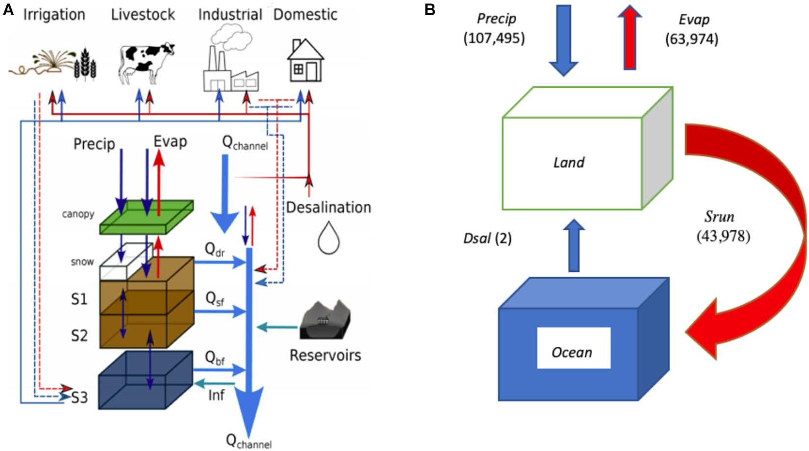
Figure 1. (A) An overview of a PCR-GLOBWB 2 grid cell from Sutanudjaja et al. (2018). S1, S2 (soil moisture storage), S3 (groundwater storage), Qdr (surface runoff), Qsf (stormflow), Qbf (baseflow), and Inf (riverbed infiltration to groundwater). (B) Simplified sketch of LWS fluxes. Precip, Precipitation; Evap, Evaporation; Dsal, Desalinated Water; SRun, Runoff (adapted from Sutanudjaja et al., 2018). Fluxes (km³yr⁻¹) shown in (B) indicate global annual mean values over the period 2000–2015.

CMIP5 Climate Models and RCP Climate Scenarios

The PCR-GLOBWB 2 model needs meteorological input data consisting of precipitation, temperature, and reference potential evaporation. To simulate LWS in this study, we forced PCR-GLOBWB 2 with the inter-sectoral impact model intercomparison experiment forcing data (Hempel et al., 2013), which consists of five global climate models (GCMs), GFDL-ESM2M, HadGEM2-ES, IPSL-CM5A-LR, MIROC-ESM-CHEM, and NorESM1-M, covering the historical period 1951–2005 and future climate period 2006–2099 (Taylor et al., 2012). For the future period, three different representative concentration pathways (RCP) are considered: RCP2.6, RCP4.5, and RCP8.5 (Masui et al., 2011; Riahi et al., 2011; Thomson et al., 2011; van Vuuren et al.,2011a,b). Note that our future projections only include the effects of climate change, while socio-economic parameters (economy, population, land use, dams) are kept constant at the level of 2005. This means that no additional dam impoundments are considered, which might result in an overestimation of LWS contribution to sea-level rise. On the other hand, water demand and therefore groundwater depletion only increases due to increased irrigation water demand which may also occur as a result of growth in human population over the twenty-first century (i.e., Raftery et al., 2012). The latter will most likely lead to an underestimation of LWS-driven sea-level rise.

Glacier Data Set and Snow Accumulation

The PCR-GLOBWB 2 is a hydrological model for all land surfaces including glaciated areas. In order to prevent double counting in terms of sea-level rise (SLR) contribution of LWS storage changes and glacier mass loss, the PCR-GLOBWB 2 data are corrected (Hock et al., 2019). We used the data from the Randolph Glacier Inventory 6.0 (Raup et al., 2007; GLIMS;NSIDC, 2018) from this we computed the glaciated area of each grid cell in the hydrological model and removed the LWS change in the output of PCR-GLOBWB 2 from those grid cells. Additionally, grid cells outside the Randolph Glacier Inventory 6.0 domain, where PCR-GLOBWB 2 simulated persistently positive snow accumulation rates over the twenty-first century, were excluded from the budget calculation of LWS change as they are artifacts resulting from a mismatch in glacier coverage in the applied data sets. The ice sheet areas of Antarctica and Greenland are also not resolved in PCR-GLOBWB 2.

Sea Level Model

After obtaining the glacier corrected fluxes from the hydrological model, we calculated the LWS differences between the periods 1986–2005 and 2081–2099 in order to compute the water mass exchange between land and ocean. GMSL rise due to this exchange is estimated by dividing the water mass exchange by the global ocean surface area. However, the water mass added from land to ocean will not cause an equal sea-level change at each location due to gravitational and rotational effects of this mass change. Therefore, we computed the pattern of sea-level change, which can be added to the patterns of glaciers, ice sheets and ocean changes to quantify the total regional sea-level rise. Detailed information in the model description and computational steps of regional sea level patterns can be found in the study of (Slangen, 2012).

Results

Temporal Evolution of LWS Over the Twentieth and Twenty-First Centuries

In order to test the model performance, we consider the historical period and compare the results from the GCM-forcing with those obtained by forcing PCR-GLOBWB 2 with observational data (Watch forcing) for the period 1958–2001 (Weedon et al., 2011). Results are shown in Figure 2.

FIGURE 2

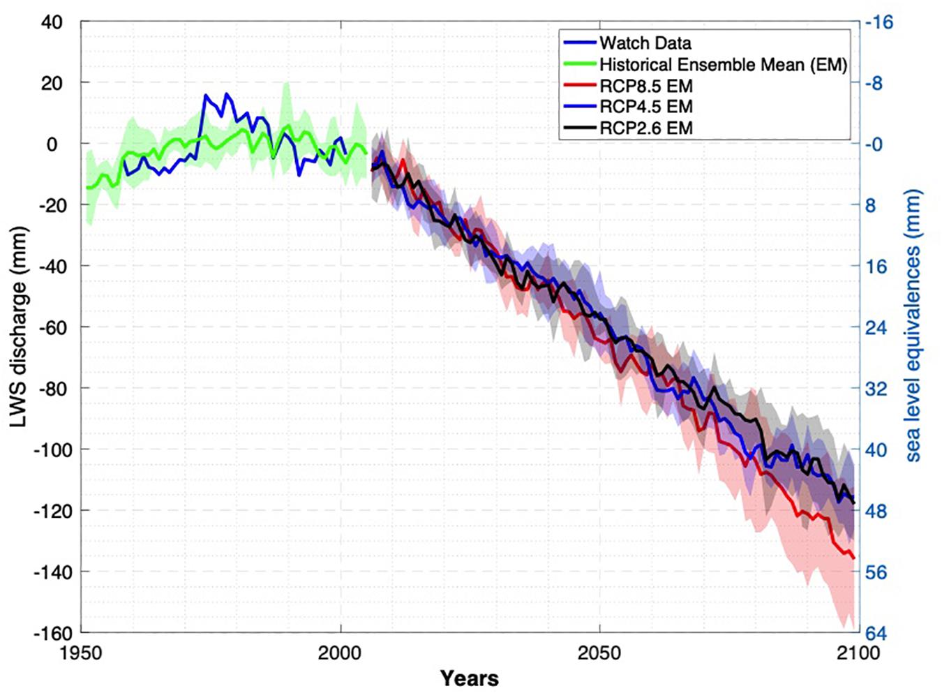
Figure 2. Change in global mean of LWS anomalies over the period 1958–2001 for which observed climate data (Watch) are available and projections with GCM-forcing over the period 1951–2099. Climate models are forced by three different RCP scenarios (RCP8.5, RCP4.5, RCP2.6) for the period 2006–2099. The mean value of observational data over the reference period 1960–1999 is subtracted from both observational data and model output. Shaded areas in scenario ensemble represent ± 1 std. from five models. Note that negative LWS change causes sea-level rise.

The general idea is that LWS storage changed from a negative contribution toward a positive contribution over the last decades which is clearly visible in the modeling results in Figure 2. Comparison of LWS anomalies from PCR-GLOBWB 2 forced by the historical ensemble and Watch observations show a consistent signal. Investigation of the interannual variability is difficult due to a lack of uncertainty for the Watch data. For the results of the LWS-driven sea-level change as presented in Table 1, the reference period 1986–2005 was chosen. This is done to make LWS changes consistent with other sea-level rise components. However, we could not use the same period for the comparison of historical time series because Watch data are only available until 2001. Figure 2 also shows that all ensemble means of different climate scenarios indicate a decrease in LWS over the twenty-first century. RCP8.5 deviates from the other scenarios (RCP4.5 and RCP2.6) in terms of the mean change over the twenty-first century. Spatial patterns of PCRGLOBWB 2 do also favorably compare with GRACE data as shown by Sutanudjaja et al. (2018). This is a result of the high resolution of the model and contrasts earlier findings by Scanlon et al. (2018) who argued that there was a discrepancy between hydrological models and GRACE data.

TABLE 1

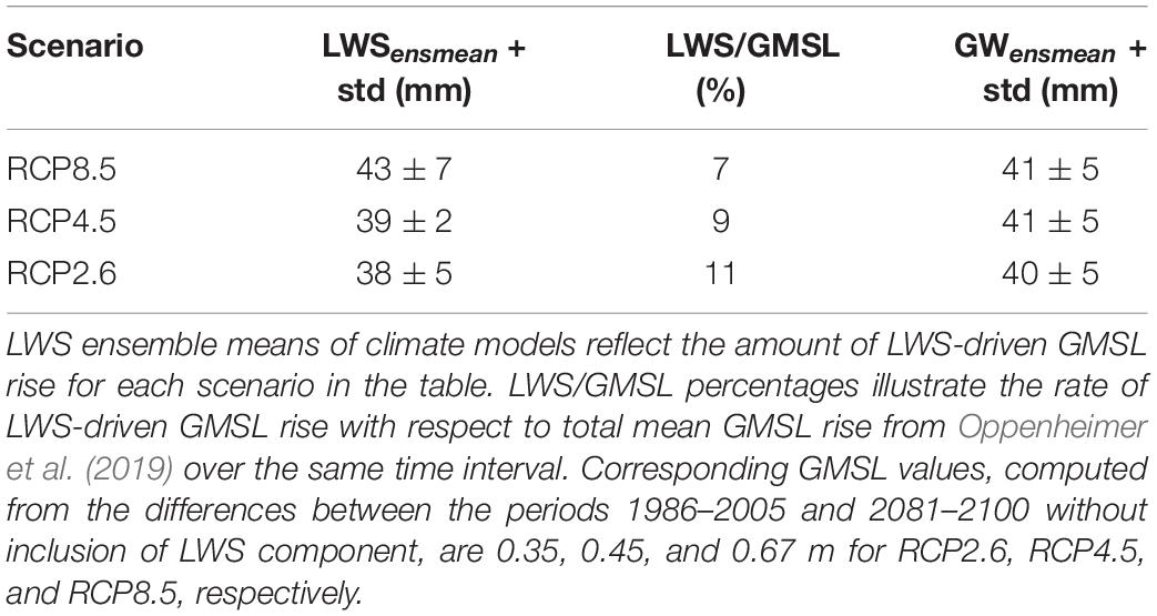
Table 1. Ensemble mean LWS-driven GMSL rise including 1 sigma, over the twenty-first century and then header in the Table LWS LWS/GMSL and GW.

Difference in LWS-Driven Sea-Level Change

By using the sea level model from Slangen (2012), we computed LWS-driven sea level patterns over the ocean in each grid-cell. Table 1 shows GMSL rise for three different climate scenarios together with the standard deviations due to the effect of LWS and non-renewable Groundwater (GW) by the end of twenty-first century relative to the mean of 1986–2005 period. Standard deviations provided in Table 1 are computed from individual results of climate models for each scenario.

LWS-driven GMSL results in a range of 38–43 mm by the end of this century, depending on the climate scenario imposed. Thereby, the LWS-driven sea-level rise corresponds to 7–11% of the total GMSL rise with respect to recently updated Special Report on the Ocean and Cryosphere in a Changing Climate (SROCC) sea level projections (Oppenheimer et al., 2019). Figure 3 displays the ensemble-mean LWS driven sea level pattern for the scenario RCP8.5. Sea level patterns of individual models for all available RCP scenarios are presented in Supplementary Figure A.

FIGURE 3

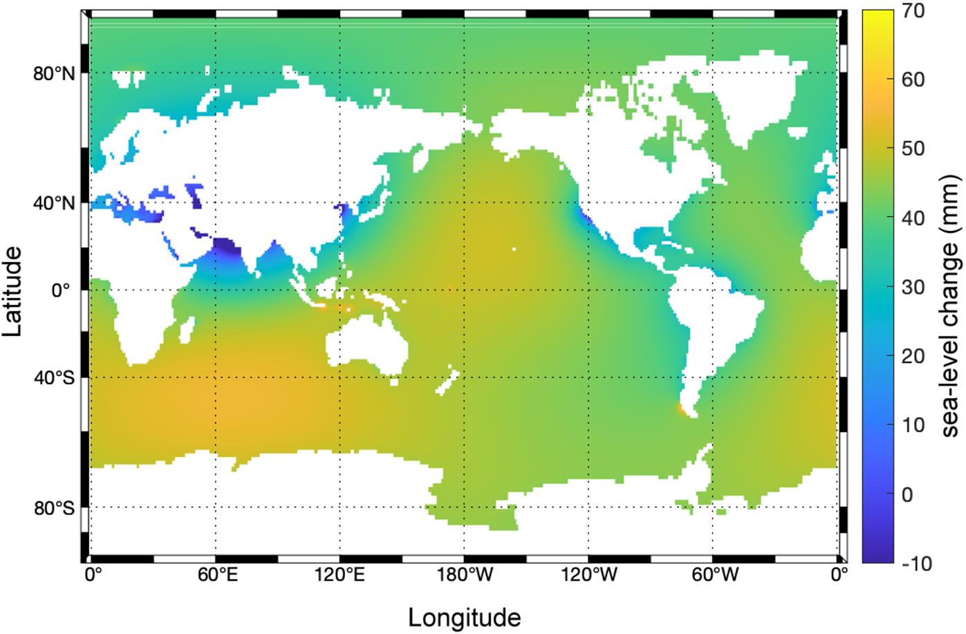
Figure 3. LWS driven regional sea-level change (mm) based on ensemble means of climate models by the end of twenty-first century under scenario RCP8.5.

Figure 3 shows a relatively large sea-level rise over the Pacific Ocean, southern coast of Africa and west coasts of Australia. Additionally, some peaks in LWS-driven sea level patterns are detected over different areas depending on the model and scenario considered. For instance, a sea level peak shows up at the south edge of South America. The reason for those peaks is discussed in the following subsection. There are also some regions, such as Mediterranean Sea, Indian coast of Asian countries and western United States, which are projected to experience some degree of sea-level fall due to the change in groundwater extraction rates by the end of twenty-first century. These changes are caused by the gravitational imprint of the abstraction of the non-renewable groundwater in those regions leading to sea level fall nearby the groundwater loss.

Attribution of LWS-Driven Sea-Level Patterns

On the one hand, the main part of regional sea level patterns over the globe is driven by extraction of non-renewable groundwater as demonstrated in Table 1. On the other hand, there are some locations experiencing sea-level peaks close to coastal areas. To study possible mechanisms behind those peaks, we focus on the possible reasons behind the positive sea level peaks close to the different coastal areas. We first analyzed the total groundwater component which includes both renewable and non-renewable groundwater layers. Positive values of the change in total groundwater storage indicate increasing groundwater recharge due to increasing rates in precipitation. Water accumulation over land due to increased amount of precipitation causes instant sea-level peaks close to coastal areas. This effect can be observed on for several regions such as north-eastern coast of South America. Figure 4 shows the different fluxes for the IPSL-CM5A-LR model under RCP8.5 as an example.

FIGURE 4

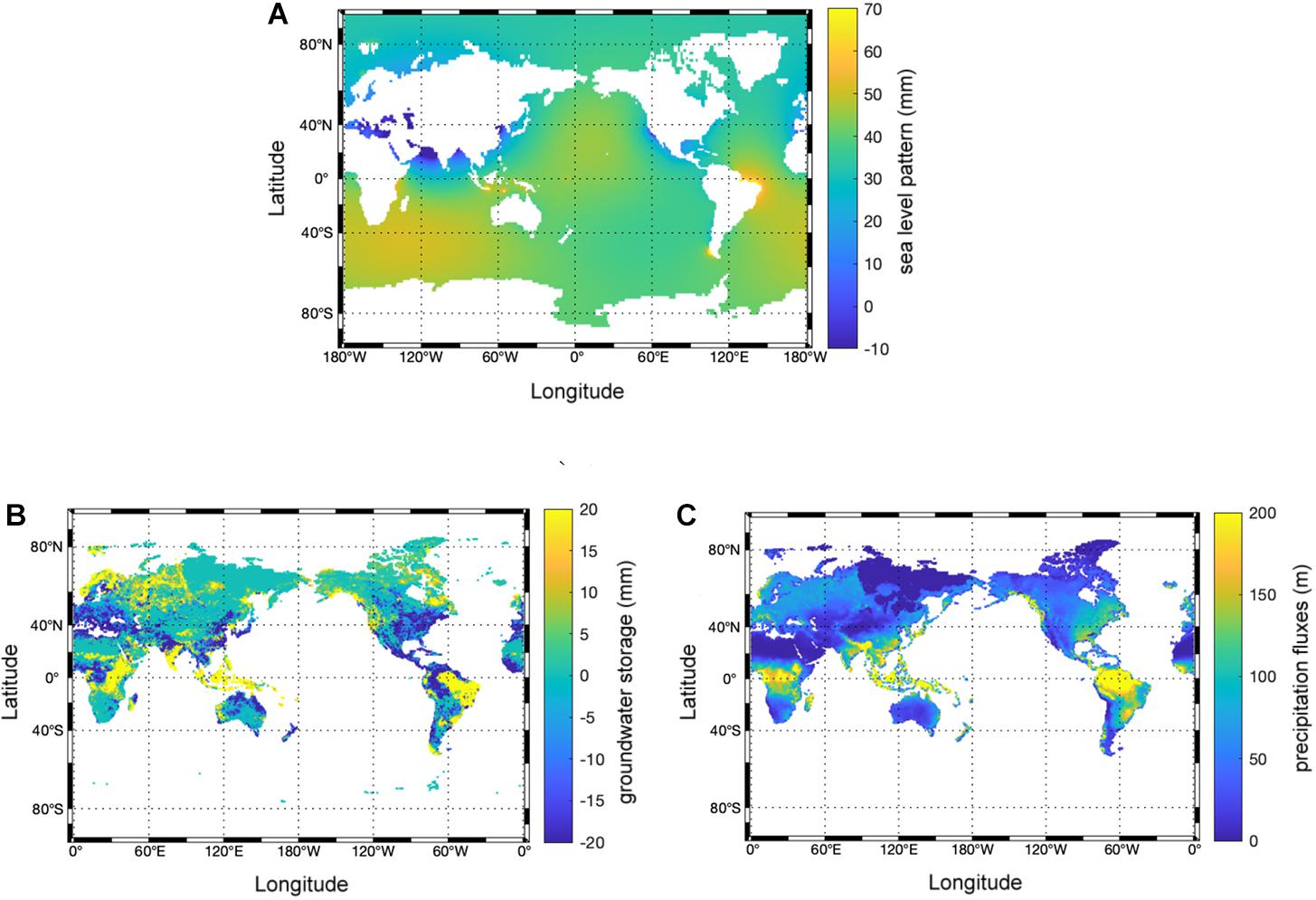
Figure 4. Change in the components forced by IPSL-CM5A-LR with RCP8.5 over the period 2081–2099 with respect to the period 1986–2005. (A) LWS-driven regional sea level pattern in mm, (B) change in groundwater storage in mm, (C) change in precipitation fluxes in m.

Figure 4A indicates that there are mainly three areas where sea level peaks are detected: the Amazon rainforest, Indonesia and Patagonia. Figure 4B shows substantial groundwater accumulation over these areas. This implies that sea level peaks in these three regions occur due to the increasing rates of groundwater recharge, owing to increase in precipitation over these three regions as shown in Figure 4C.

Factors Causing Differences Between Models in Projecting Regional Sea-Level Changes

The sea level patterns of the ensemble means for different scenarios are very similar. In contrast, differences between models for the same scenario are large, especially for RCP8.5. We refer reader to see Supplementary Figure A which provides detailed information on LWS-driven regional sea level changes (mm) for five individual climate models based on three R by the end of twenty-first century. Figure 5 shows the maximum difference among the models and show the differences in precipitation, evaporation and runoff fluxes between models for this scenario.

FIGURE 5

Figure 5. Model output differences (m) between highest value and lowest value in each grid cell for precipitation (A), evaporation (B), and runoff (C) fluxes based on the scenario RCP8.5. For a given flux, model outputs represent the mean changes in each grid-cell over the period 1986–2005 to 2081–2099.

The figure indicates large differences in precipitation, evaporation and runoff fluxes over several regions. The differences in these fluxes over substantial parts of tropical Africa, for Asian countries directly connected to the Indian Ocean, the northern and eastern coasts of Australia, eastern South America including the Amazon forest and central America are responsible for the differences in regional sea-level change. Differences in evaporation rates, tend to be small in comparison to precipitation and runoff fluxes for these areas. The maps of precipitation and runoff fluxes point toward non-negligible inter-GCM differences over south-western side of Chile, the eastern coasts of north America, the northern part of New Zealand and north-western Europe and inner Russia.

In principle, we should be able to link the discrepancies in fluxes suggested by different climate models to discrepancies in sea level patterns. However, such an analysis is far from straightforward, since the sea level model calculates sea level patterns based on the interference of complex spatial patterns of mass changes. On the other hand, we can attribute the sea level peaks displayed in a specific model using a similar analysis as implemented in a previous subsection. For instance, a peak in sea-level rise along the coast of north-eastern South America is observed only when forced with output from the model IPSL-CM5A-LR. This sea level pattern most likely results from the fact that the RCP8.5 projection with IPSL-CM5A-LR produces a precipitation peak that strongly deviates from the other GCMs. Similarly, we can argue that the individual peaks in sea-level change differences between models along the eastern coast of India, result from very different patterns in precipitation and runoff for the model HadGEM2-ES.

Differences Among Scenarios and Models

To compare the differences in sea level patterns, we analyzed the differences between models and between scenarios separately. Figure 6 shows the result of this comparison.

FIGURE 6

Figure 6. Sea level changes (mm) between highest value and lowest value between scenarios for a given model (A), and between models for a given scenario (B). In panel (A) models are ordered alphabetically and in panel (B) scenarios are ordered from high-end to low-end emission scenarios from top to bottom.

Figure 6A illustrates that the differences in sea level patterns do not show substantial deviations for a given model among the different climate scenarios. However, the global pattern of HadGEM2-ES differs from the other four models and NorESM1-M produces some peaks along the coasts of Indonesia. Figure 6B shows the differences between the maximum and minimum values among the climate models for a given scenario, indicating that differences due to the use of different models are non-negligible in some regions. This is particularly relevant along the coasts of India for all scenarios. There are also some regions such as areas close to the north coast of Brazil, the Indian coasts and Java island where the different models project particularly large differences in sea-level change, up to 100 mm for only the RCP8.5. The global average model differences are larger for RCP2.6 (12 mm) than for RCP4.5 (8 mm). Individual GMSL change values for the individual climate models and RCPs are provided in the Supplementary Table A. Large model differences are mainly detected only along the Indian coasts. In summary, Figure 6 shows that the magnitude in sea level pattern differences due to models is larger than the differences due to climate scenarios.

Discussion

Previous estimates of the contribution of LWS to sea-level change rely mainly on non-renewable groundwater abstraction rates (Konikow, 2011; Wada et al., 2012). Although non-renewable groundwater abstraction is a dominant factor in comparison to the effect of other fluxes, including the effects of climate-related LWS change was shown to be regionally important as well and quite different between climate models.

By extrapolating the dam construction (Wada et al., 2012), projected LWS-driven sea-level rise over the twenty-first century. Their results indicated that global sea-level rise will be around 73 mm. It suggested a relatively high contribution of LWS to sea-level rise. However, this should be viewed as a high estimate of LWS-driven sea-level rise, since natural LWS change was not included in this study and future projections of LWS were basically the extrapolation of water impoundment reserved by the dams and does not provide regional patterns of sea level. Here, for the first time, we include climate-driven change in LWS by considering two different future climate scenarios and provide regional sea-level patterns driven by a state-of-the-art global hydrology and water resources model, PCR-GLOBWB 2.

Regarding the regional sea level patterns, a crucial assumption in computing LWS is that the groundwater storage is simplified by a linear reservoir concept with no lateral groundwater flow which could cause a limited interaction of groundwater and surface water bodies (see Sutanudjaja et al., 2014) for a PCR-GLOBWB 2 version that includes a full groundwater flow components). This may lead to further regional changes which need to be considered in a future work. A more important additional shortcoming is the lack of feedback from the hydrological model to the climate model. These feedbacks may result in increasing rates in precipitation over land in areas with groundwater-based irrigation which reduces the transport of pumped groundwater from the land to the ocean (e.g., Deangelis et al., 2010). This simplification may cause a small overestimation of LWS-driven GMSL rise (Wada et al., 2016).

The influence of possible social and economic changes, as portrayed in the Shared Socio-economic Pathways (SSPs) (Riahi et al., 2017), on groundwater demand and withdrawal are not included in this study. On the one hand, including different SSPs in projecting LWS will likely lead to additional changes in groundwater depletion and consequential regional sea-level increase. On the other hand, growth in human population will increase the demand on energy supply. This demand may cause impoundment of substantial amount of water behind dams, hence, lower the LWS discharge over the twenty-first century.

Conclusion

In this study, we quantified the contribution of LWS change to regional sea-level rise by considering five different climate models forced by three different climate scenarios over the twenty-first century. Our conclusions are as follows:

- Simulations under different climate scenarios indicate a contribution range of LWS change between 38 mm (11%) and 43 mm (7%) to GMSL rise and indicates up to 60% higher than global average of LWS-driven sea-level rise in some regions for the twenty-first century.

1. The amount of groundwater extraction rates over the Asian continental countries along the Indian ocean, the eastern coast of China and the western coast of United States play a crucial role in driving LWS-affected GMSL rise. However, regional increases in precipitation may have a non-negligible effect on driving regional sea level, especially over the tropical regions.

2. Differences between models in simulating precipitation result in sea level patterns for individual models for an identical climate scenario. The variation in LWS-driven sea level patterns depends more on the climate model used than on the scenario used.

3. Ensemble mean projections indicate that the islands in the Northern Pacific will be exposed to the largest sea-level rise resulting from a change of LWS.

Data Availability Statement

The raw data supporting the conclusions of this article will be made available by the authors, without undue reservation, to any qualified researcher.

Author Contributions

SK did the analysis. SK and ES wrote the manuscript. ES performed the PCR-GLOBWB 2 simulations. EL, MB, and RV contributed to the discussion, review, and editing of the article. RV supervised the project. All authors conceptualized and framed this research article.

Funding

SK received funding from the Netherlands Polar Programme and the Water, Climate and Future Deltas program of Utrecht University. EL was financially supported by the INSeaption project which is part of ERA4CS and ERA-NET initiative by JPI Climate and funded by NWO.

Conflict of Interest

The authors declare that the research was conducted in the absence of any commercial or financial relationships that could be construed as a potential conflict of interest.

Acknowledgments

ES and MB acknowledge the funding from World Resources Institute under the Aqueduct Flood Analyzer project that allows PCR-GLOBWB 2 simulation used in this study. The PCR-GLOBWB 2 simulation was carried out on the Dutch national e-infrastructure with the support of SURF Cooperative.

Supplementary Material

The Supplementary Material for this article can be found online at: https://www.frontiersin.org/articles/10.3389/feart.2021.627648/full#supplementary-material

References

Chao, B.F., Wu, Y. H., and Li, S. Y. (2008). Impact of artificial reservoir water impoundment on global sea level. Science 320, 212–214. doi: 10.1126/science.1154580

PubMed Abstract | CrossRef Full Text | Google Scholar

Church, J. A., Clark, P. U., Cazenave, A., Gregory, J. M., Jevrejeva, S., Levermann, A., et al. (2013). Sea level change. Climate Change 2013: The Physical Science Basis. Contribution of Working Group I to the Fifth Assessment. Geneva: IPCC. 1137–1216.

Google Scholar

Dangendorf, S., Marcos, M., Wöppelmann, G., Conrad, C. P., Frederikse, T., Riva, R., et al. (2017). Reassessment of 20th century global mean sea level rise. Proc. Natl. Acad. Sci. U. S. A., 114, 5946–5951. doi: 10.1073/pnas.1616007114

PubMed Abstract | CrossRef Full Text | Google Scholar

Deangelis, A., Dominguez, F., Fan, Y., Robock, A., Kustu, M. D., and Robinson, D. (2010). Evidence of enhanced precipitation due to irrigation over the great plains of the united states. J. Geophys. Res. Atmos. 115, doi: 10.1029/2010JD013892

CrossRef Full Text | Google Scholar

Dieng, H. B., Champollion, N., Cazenave, A., Wada, Y., Schrama, E., and Meyssignac, B. (2015). Total land water storage change over 2003-2013 estimated from a global mass budget approach. Environ. Res. Lett. 10:124010. doi: 10.1088/1748-9326/10/12/124010

CrossRef Full Text | Google Scholar

Fettweis, X., Franco, B., Tedesco, M., Van Angelen, J. H., Lenaerts, J. T. M., Van Den Broeke, M. R., et al. (2013). Estimating the Greenland ice sheet surface mass balance contribution to future sea level rise using the regional atmospheric climate model MAR. Cryosphere, 7, 469–489. doi: 10.5194/tc-7-469-2013

CrossRef Full Text | Google Scholar

Frederikse, T., Landerer, F., Caron, L., Adhikari, S., Parkes, D., Vincent, W.H, et al. (2020). The causes of sea-level rise since 1900. Nature 584, 393–397. doi:Google Scholar

GLIMS;NSIDC (2018). Global land ice measurement from space glacier database. Co,piled and made available by the international GLIMS community and the National Snow and Ice Data Center.

Google Scholar

Gornitz, V. (2001). Chapter 5 impoundment, groundwater mining, and other hydrologic transformations: Impacts on global sea level rise. Int. Geophys. 75, 97–119. doi: 10.1016/S0074-6142(01)80008-5

CrossRef Full Text | Google Scholar

GRDC (2014): The Global Runoff Data Centre (GRDC): The Global Runoff Database and River Discharge Data, Available Online at: http://www.bafg.de/GRDC (Accessed 17 April 2014), n.d.

Google Scholar

Gregory, J. M., White, N. J., Church, J. A., Bierkens, M. F. P., Box, J. E., and Van Den Broeke, M. R. (2013). Twentieth-century global-mean sea level rise: Is the whole greater than the sum of the parts? J. Clim. 26, 4476–4499. doi: 10.1175/JCLI-D-12-00319.1

CrossRef Full Text | Google Scholar

Hay, C., Morrow, E., Kopp, R., and Mitrovica, J. (2015). Probabilistic reanalysis of twentieth-century sea-level rise. Nature, 517, 481–484. doi: 10.1038/nature14093

PubMed Abstract | CrossRef Full Text | Google Scholar

Hempel, S., Frieler, K., Warszawski, L., Schewe, J., and Piontek, F. (2013). A trend-preserving bias correction & the ISI-MIP approach. Earth Syst. Dyn. 4, 219–236. doi: 10.5194/esd-4-219-2013

CrossRef Full Text | Google Scholar

Hock, R., Bliss, A., Marzeion, B. E. N., Giesen, R. H., Hirabayashi, Y., and Huss, M. (2019). GlacierMIP-A model intercomparison of global-scale glacier mass-balance models and projections. J. Glaciol., 65, 453–467. doi: 10.1017/jog.2019.22

CrossRef Full Text | Google Scholar

Jenkins, A., and Holland, D. (2007). Melting of floating ice and sea level rise. Geophys. Res. Lett. 34, 1–5. doi: 10.1029/2007GL030784

CrossRef Full Text | Google Scholar

Katsman, C. A., Hazeleger, W., Drijfhout, S. S., Van Oldenborgh, G. J., and Burgers, G. (2008). Climate scenarios of sea level rise for the northeast atlantic ocean: a study including the effects of ocean dynamics and gravity changes induced by ice melt. Clim. Change 91, 351–374. doi: 10.1007/s10584-008-9442-9

CrossRef Full Text | Google Scholar

Konikow, L. F. (2011). Contribution of global groundwater depletion since 1900 to sea-level rise. Geophys. Res. Lett. 38, 1–5. doi: 10.1029/2011GL048604

CrossRef Full Text | Google Scholar

Marzeion, B., Jarosch, A. H., and Hofer, M. (2012). Past and future sea-level change from the surface mass balance of glaciers. Cryosphere 6, 1295–1322. doi: 10.5194/tc-6-1295-2012

CrossRef Full Text | Google Scholar

Masui, T., Matsumoto, K., Hijioka, Y., Kinoshita, T., Nozawa, T., Ishiwatari, S., et al. (2011). An emission pathway for stabilization at 6 Wm-2 radiative forcing. Clim. Change 109, 59–76. doi: 10.1007/s10584-011-0150-5

CrossRef Full Text | Google Scholar

Milly, P. C. D., Cazenave, A., and Gennero, C. (2003). Contribution of climate-driven change in continental water storage to recent sea-level rise. Proc. Natl. Acad. Sci. 100, 13158–13161. doi: 10.1073/pnas.2134014100

PubMed Abstract | CrossRef Full Text | Google Scholar

Milly, P. C. D. C., Cazenave, A., Famiglietti, J. S., Gornitz, V., Laval, K., Lettenmaier, D. P., et al. (2010). Terrestrial water - storage contributions to sea - level rise and variability. In Understanding Sea−Level Rise and Variability. (eds) J. A. Church, P. L. Woodworth, T. Aarup, and W. S. Wilson Oxford: Blackwell Publishing Ltd. 226–255.

Google Scholar

Ngo-Duc, T., Laval, K., Polcher, J., Lombard, A., and Cazenave, A. (2005). Effects of land water storage on global mean sea level over the past half century. Geophys. Res. Lett., 32, 1–4. doi: 10.1029/2005GL022719

CrossRef Full Text | Google Scholar

Oppenheimer, M., Glavovic, B.C., Hinkel, J., Van de Wal, R., Magnan, A.K., Abd-Elgawad, A., et al. (2019). Sea Level Rise and Implications for Low-Lying Islands, Coasts and Communities. In: IPCC Special Report on the Ocean and Cryosphere in a Changing Climate. (eds) H.-O. Pörtner, D.C. Roberts, V. Masson-Delmotte, P. Zhai, M. Tignor, E. Poloczanska, et al.. Geneva: Intergovernmental Panel on Climate Change. 126.

Google Scholar

Peltier, W. R. (2001). Global glacial isostatic adjustment and modern instrumental records of relative sea level history. Int. Geophys., 75, 65–95

Google Scholar

Pokhrel, Y. N., Hanasaki, N., Yeh, P. J. F., Yamada, T. J., Kanae, S., Oki, T., et al. (2012). Model estimates of sea-level change due to anthropogenic impacts on terrestrial water storage. Nat. Geosci. 5, 389–392. doi: 10.1038/ngeo1476

CrossRef Full Text | Google Scholar

Raftery, A. E., Li, N., Ševc̀íková, H., Gerland, P., and Heilig, G. K. (2012). Bayesian probabilistic population projections for all countries. Proc. Natl. Acad. Sci. U. S. A. 109, 13915–13921. doi: 10.1073/pnas.1211452109

PubMed Abstract | CrossRef Full Text | Google Scholar

Raup, B. H., Racoviteanu, A., Khalsa, S. J. S., Helm, C., Armstrong, R., Arnaud, Y., et al. (2007). The GLIMS geospatial glacier database: a new tool for studying glacier change. Glob. Planet. Change, 56, 101–110. doi: 10.1016/j.gloplacha.2006.07.018

CrossRef Full Text | Google Scholar

Reager, J. T., Gardner, A. S., Famiglietti, J. S., Wiese, D. N., Eicker, A., Lo, M. H., et al. (2016). : A decade of sea level rise slowed by climate-driven hydrology. Science 351, 699–703., doi: 10.1126/science.aad8386

PubMed Abstract | CrossRef Full Text | Google Scholar

Riahi, K., Fricko, O., Lutz, W., Cuaresma, J. C., KC, S., Rao, S., et al. (2017). The shared socioeconomic pathways and their energy, land use, and greenhouse gas emissions implications: an overview. Glob. Environ. Chang., 42, 153–168. doi: 10.1016/j.gloenvcha.2016.05.009

CrossRef Full Text | Google Scholar

Riahi, K., Rao, S., Krey, V., Cho, C., Chirkov, V., Fischer, G., et al. (2011). RCP 8.5-A scenario of comparatively high greenhouse gas emissions. Clim. Change, 109, 33–57. doi: 10.1007/s10584-011-0149-y

CrossRef Full Text | Google Scholar

Sahagian, D. (2000). Global physical effects of anthropogenic hydrological alterations: sea level and water redistribution. Glob. Planet. Change, 25, 39–48. doi: 10.1016/S0921-8181(00)00020-5

CrossRef Full Text | Google Scholar

Sahagian, D. L., Schwartz, F. W., and Jacobs, D. K. (1994). Direct anthropogenic contributions to sea level rise in the twentieth century. Nature, 367, 54–57. doi: 10.1038/367054a0

CrossRef Full Text | Google Scholar

Scanlon, B. R., Zhang, Z., Save, H., Sun, A. Y., Schmied, H. M., Van Beek, L. P. H., et al. (2018). Global models underestimate large decadal declining and rising water storage trends relative to GRACE satellite data. Proc. Natl. Acad. Sci. U. S. A. 115, E1080–E1089. doi: 10.1073/pnas.1704665115

PubMed Abstract | CrossRef Full Text | Google Scholar

Slangen, A. (2012). Modelling Regional Sea-Level Changes In Recent Past And Future. Netherland: Institute for Marine and Atmospheric research Utrecht.

Google Scholar

Sutanudjaja, E. H., Van Beek, L. P. H., De Jong, S. M., Van Geer, F. C., and Bierkens, M. F. P. (2014). Calibrating a large-extent high-resolution coupled groundwater-land surface model using soil moisture and discharge data. Water Resour. Res. 50, 687–705. doi: 10.1002/2013WR013807

CrossRef Full Text | Google Scholar

Sutanudjaja, E. H., Van Beek, R., Wanders, N., Wada, Y., Bosmans, J. H. C., Drost, N., et al. (2018). PCR-GLOBWB 2: A 5 arcmin global hydrological and water resources model. Geosci. Model Dev. 11, 2429–2453. doi: 10.5194/gmd-11-2429-2018,2018

PubMed Abstract | CrossRef Full Text | Google Scholar

Taylor, K. E., Stouffer, R. J., and Meehl, G. A. (2012). An overview of CMIP5 and the experiment design. Bull. Am. Meteorol. Soc. 93, 485–498. doi: 10.1175/BAMS-D-11-00094.1

CrossRef Full Text | Google Scholar

Taylor, R. G., Scanlon, B., Döll, P., Rodell, M., Van Beek, R., Wada, Y., et al. (2013). Ground water and climate change. Nat. Clim. Chang. 3, 322–329. doi: 10.1038/nclimate1744

CrossRef Full Text | Google Scholar

Thomson, A. M., Calvin, K. V., Smith, S. J., Kyle, G. P., Volke, A., Patel, P., et al. (2011). RCP4.5: a pathway for stabilization of radiative forcing by 2100. Clim. Change, 109, 77–94. doi: 10.1007/s10584-011-0151-4

CrossRef Full Text | Google Scholar

Van Beek, L. P. H., Wada, Y., and Bierkens, M. F. P. (2011): Global monthly water stress: 1. Water balance and water availability. Water Resour. Res., 47, doi: 10.1029/2010WR009791

CrossRef Full Text. | Google Scholar

van Vuuren, D. P., Edmonds, J., Kainuma, M., Riahi, K., Thomson, A., Hibbard, K., et al. (2011b). The representative concentration pathways: an overview. Clim. Change, 109, 5–31. doi: 10.1007/s10584-011-0148-z

CrossRef Full Text | Google Scholar

van Vuuren, D. P., Stehfest, E., den Elzen, M. G. J., Kram, T., van Vliet, J., Deetman, S., et al. (2011a). RCP2.6: Exploring the possibility to keep global mean temperature increase below 2°C. Clim. Change, 109, 95–116. doi: 10.1007/s10584-011-0152-3

CrossRef Full Text | Google Scholar

Wada, Y., Lo, M. H., Yeh, P. J. F., Reager, J. T., Famiglietti, J. S., Wu, R. J., et al. (2016). Fate of water pumped from underground and contributions to sea-level rise. Nat. Clim. Chang. 6, 777–780. doi: 10.1038/nclimate3001

CrossRef Full Text | Google Scholar

Wada, Y., Van Beek, L. P. H., Sperna Weiland, F. C., Chao, B. F., Wu, Y. H., Bierkens, M. F. P., et al. (2012). Past and future contribution of global groundwater depletion to sea-level rise. Geophys. Res. Lett. 39, 1–6. doi: 10.1029/2012GL051230

CrossRef Full Text | Google Scholar

Weedon, G. P., Gomes, S., Viterbo, P., Shuttleworth, W. J., Blyth, E., Österle, H., et al. (2011). Creation of the watch forcing data and its use to assess global and regional reference crop evaporation over land during the twentieth century. J. Hydrometeorol. 12, 823–848. doi: 10.1175/2011jhm1369.1

CrossRef Full Text | Google Scholar

Wiese, D. N. (2015). GRACE monthly global water mass grids netcdf release 5.0, PO.DAAC.

Google Scholar