Evaluating Accuracy of HY-2A/GM-Derived Gravity Data With the Gravity-Geologic Method to Predict Bathymetry

Introduction

Ocean depth plays a very important role in marine geology, geophysics and geodesy, such as the study of earth’s plate tectonics, changes of ocean currents and tides, and navigation of ships. Bathymetry prediction mainly includes satellite remote sensing, sonar images and satellite altimetry gravity anomalies.

Although satellite remote sensing (Jay and Guillaume, 2014) has advantages in economy and flexibility, its accuracy needs to be improved. High-resolution seafloor topography prediction of sonar images is achieved with the shape from shaping (Coiras et al., 2007), which needs to be constrained by external bathymetry. In the past 50 years, great progress has been made the technical performance of satellite altimetry technology (e.g., Born et al., 1979; Cheney et al., 1986; Francis et al., 1995; Hwang et al., 2002; Guo et al., 2014, 2015, 2016), and its measurement accuracy and resolution (Hsiao et al., 2016) have been greatly improved. The technology has made a significant contribution to the satellite altimetry-derived ocean gravity field (e.g., Sandwell and Smith, 1997, 2009; Hwang et al., 2006, 2014; Guo et al., 2010; Zhu et al., 2019, 2020; Li et al., 2020) and to the study of bathymetry prediction (e.g., Calmant and Baudry, 1996; Luo et al., 2002).

Gravity prediction of bathymetry mainly includes the gravity-geologic method (GGM) (Ibrahim and Hinze, 1972; Adams and Hinze, 1990), admittance function method (Dorman and Lewis, 1970; Watts, 1978) and least-squares collocation method (Hwang, 1999). The ship-borne bathymetry data is relatively sparse (Smith and Sandwell, 1994). Compared with the other two methods, GGM has the advantage of using sparse ship-borne bathymetry to obtain depth model. A comparison with Smith and Sandwell model shows that GGM has an advantage with short wavelength components (≤12 km) which are sensitive to bathymetry variations (Kim et al., 2010).

Gravity-geologic method has been used to predict bathymetry in southern Greenland, southern Alaska (Hsiao et al., 2011), the southern Western Pacific Emperor Seamount (Hu et al., 2012) and the central South China Sea (Ouyang et al., 2014). The density contrast between seawater and ocean bottom topography has a large impact on the accuracy of bathymetry prediction. Although the accuracy of GGM bathymetry using the density contrast obtained with the downward continuation method (Hwang, 1999; Kim et al., 2010, 2011) reaches 40 m (Kim et al., 2010), the density contrast is quite different from the theoretical value of 1.64 g/cm³ and therefore loses its physical significance. The density contrast obtained with the iterative method (Silva et al., 2006; Kim et al., 2010; Hu et al., 2012) is close to the theoretical value, achieving good test results.

At present, bathymetry prediction is generally based on existing gravity anomalies, or the gravity anomalies obtained by combining multi-satellite data. There are relatively few researches on the application of HY-2A/GM-derived gravity anomalies in bathymetry prediction. The objective of this study is to apply GGM to estimation of the bathymetry of the test areas in the South China Sea with HY-2A/GM-derived gravity anomalies. In this paper, differences are analyzed among GGM bathymetry, ship-borne bathymetry and other depth models (e.g., SRTM15+V2.0 model and GEBCO 2020 model). Geological structures, gravity anomalies and other factors affecting the accuracy of GGM bathymetry are discussed, and the relationship is studied between relative accuracy of GGM bathymetry and variation of depth. The results show that HY-2A/GM-derived gravity anomalies can be used to predict bathymetry, and GGM can be effectively applied to areas with sparse ship-borne bathymetry.

The Gravity-Geologic Method

The gravity-geologic method (GGM) is originally proposed by Ibrahim and Hinze (1972). Because the density difference between seawater and ocean bottom topography is large, GGM is suitable for predicting bathymetry with gravity anomalies. The estimation of ocean bottom topography from gravity has the single contact restoration problem (Grant and West, 1965). Therefore, a simple Bouguer correction formula (linearized contact restoration problem) is adopted. The ambiguity involves the choice of depth, D. To minimize the ambiguity, the control points data are used. However, in a linearized contact surface problem, D happens to be the mean depth. In data processing, the gravity anomaly is linearized into the residual gravity field produced by local bedrock variations and the regional gravity field generated by deeper mass variations. Then, the residual gravity field is used to predict the final depth. The calculation process is as follows.

Gravity anomalies are divided into the residual gravity anomaly and the regional gravity anomaly, i.e.:

$$g_{inv}=g_{reg}+g_{res}(1)$$

where g_inv means gravity anomaly, and g_res and g_reg denote residual gravity anomaly and regional gravity anomaly, respectively.

The residual gravity anomaly ($g_{res}^j$) can be presented as:

$$g_{res}^j=2\mathrm{\pi }G\mathrm{\Delta }\mathrm{\rho }(H_j-D)(2)$$

where $g_{res}^j$ denotes the residual gravity anomaly at the point j; G is the gravitational constant, and Δρ is the optimal density contrast between seawater and ocean bottom topographic mass, called density contrast.H_j is the control point j and D is the reference depth, which is usually referenced to the deepest depth of the control points.

Furthermore, the residual gravity anomaly ($g_{res}^j$) can be subtracted from the gravity anomaly ($g_{inv}^j$) to obtain the regional gravity anomaly ($g_{reg}^j$) at the point j. It can be given by:

$$g_{reg}^j=g_{inv}^j-g_{res}^j(3)$$

After that, the regional gravity anomaly ($g_{reg}^j$) is gridded to create a reference gravity anomaly grid (g_reg) and the regional gravity anomaly is obtained by cubic spline interpolation at the check points ($g_{reg}^i$). Then, the residual gravity anomaly ($g_{res}^i$) is obtained by:

$$g_{res}^i=g_{inv}^i-g_{reg}^i(4)$$

Finally, bathymetry is calculated by:

$$H_i=\frac{g_{res}^i}{2\mathrm{\pi }G\mathrm{\Delta }\mathrm{\rho }}+D(5)$$

Figure 1 shows the flow chart of GGM operation steps and the iterative method to solve density contrast. First, initialized value of the density contrast is given, and ocean depth is obtained with GGM. Then, the control points depth is obtained with cubic spline interpolation. And the standard deviation and the correlation coefficient are compared between the GGM bathymetry and the ship-borne bathymetry difference at control points. Finally, if the difference is not judged to be the smallest, the assignment continues to be performed; Otherwise, the value is the suitable density contrast.

FIGURE 1

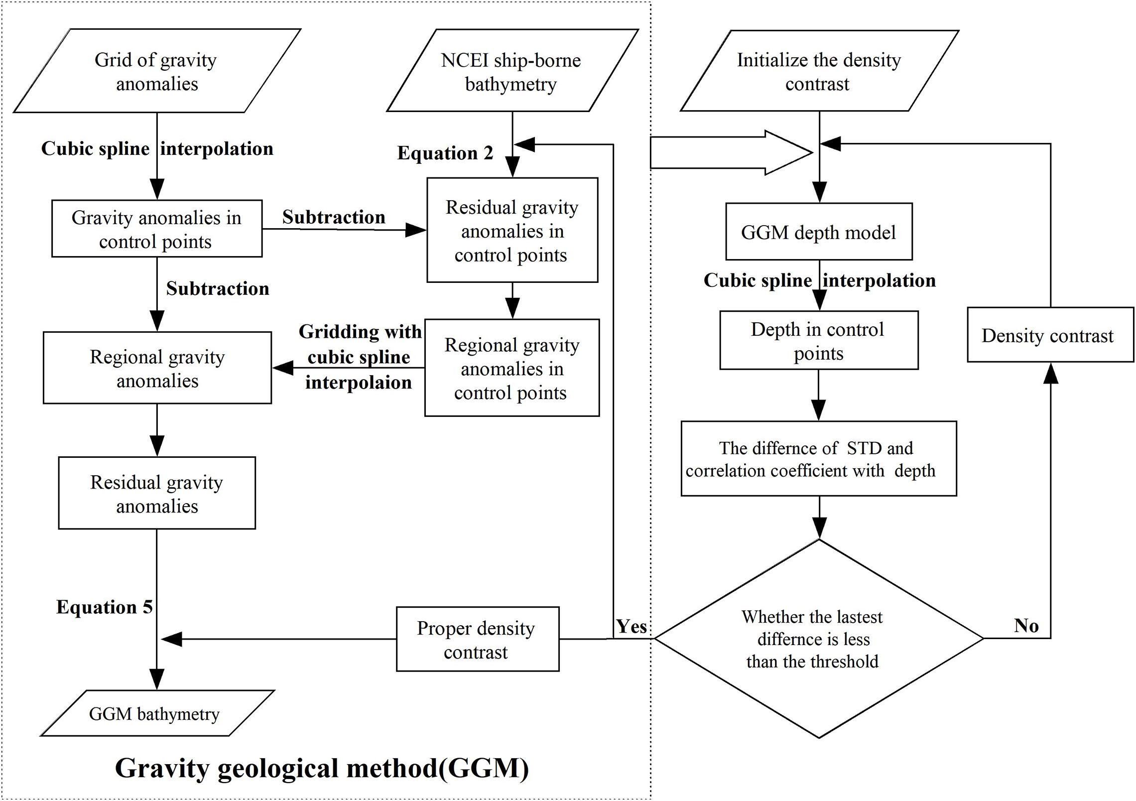
Figure 1. Flow chart of the gravity-geologic method (GGM) and iterative method.

Test Area

The South China Sea (SCS), as the western marginal sea of the Pacific Ocean, lies among the Eurasian plate, the Pacific plate and the Indian Ocean plate. Its geological structures and topography are complex. The overall topography inclines from the periphery to the center, with continental shelf, continental slope, abyssal basin and other landform types transitioning from shallow to deep (Qiu et al., 2016). Different topography and landforms constitute the basic features of the SCS geology.

The SCS is taken as the research area, and the characteristics of GGM bathymetry prediction under different geological structures can be well analyzed. The three test areas of A (112–119°E, 16–20°N), B (111–118°E, 12–15°N) and C (109–115°E, 6–10°N). Figure 2 shows the locations of the test areas.

FIGURE 2

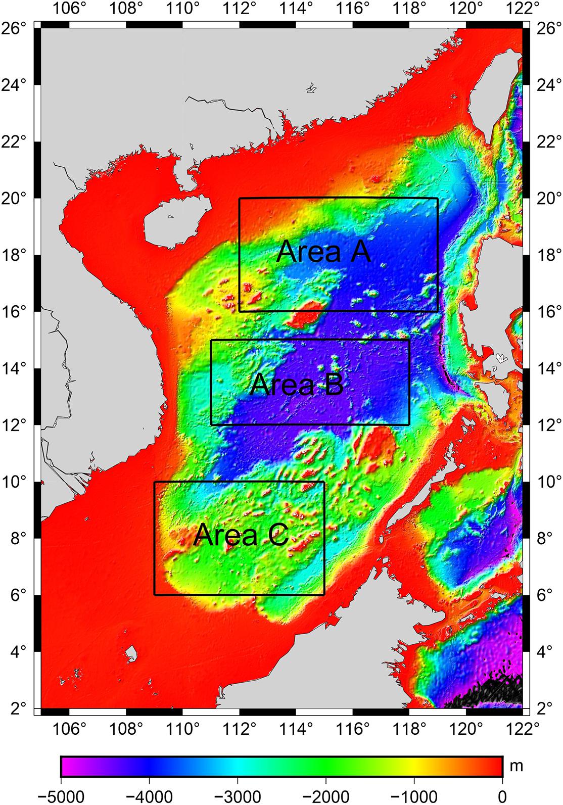
Figure 2. Seafloor topography of the SCS. Locations of the test areas (Areas A, B, and C) are shown in the background map of GEBCO 2020 bathymetry model.

Data

HY-2A/GM-derived Gravity Anomaly

The gravity anomalies on 1′ × 1′ grids in the SCS (105–122°E, 2–26°N) are obtained from altimetry data of geodetic mission (GM) of HY-2A (which is China’s first satellite altimeter mission launched in August 2011). The GM of HY-2A was carried out after the orbit modification on March 30, 2016. The cycle of GM increases from 14 d to 168 days and its working range is 81°S-81°N. The HY-2A/GM altimeter data of Level 2 Plus (L2P) products [Centre National d’Etudes Spatiales (CNES), 2017] sampled at a frequency of 1 Hz from March 30, 2016 to August 22, 2018 are selected as the research data. First, sea surface heights (SSHs) of HY-2A/GM are pre-processed by correction and gross error elimination. Then pre-processed SSHs are used to calculate along-track geoid gradients, from which residual geoid gradients can be obtained by removing geoid gradients of EGM2008. Finally, residual gravity anomalies on 1′ × 1′ grids are derived from residual geoid gradients with the least-squares collocation method whose calculation window radius is 0.5°. The final gravity anomaly model (Zhu et al., 2019) is obtained from residual gravity anomalies by restoring gravity anomalies of EGM2008, as is shown in Figure 3.

FIGURE 3

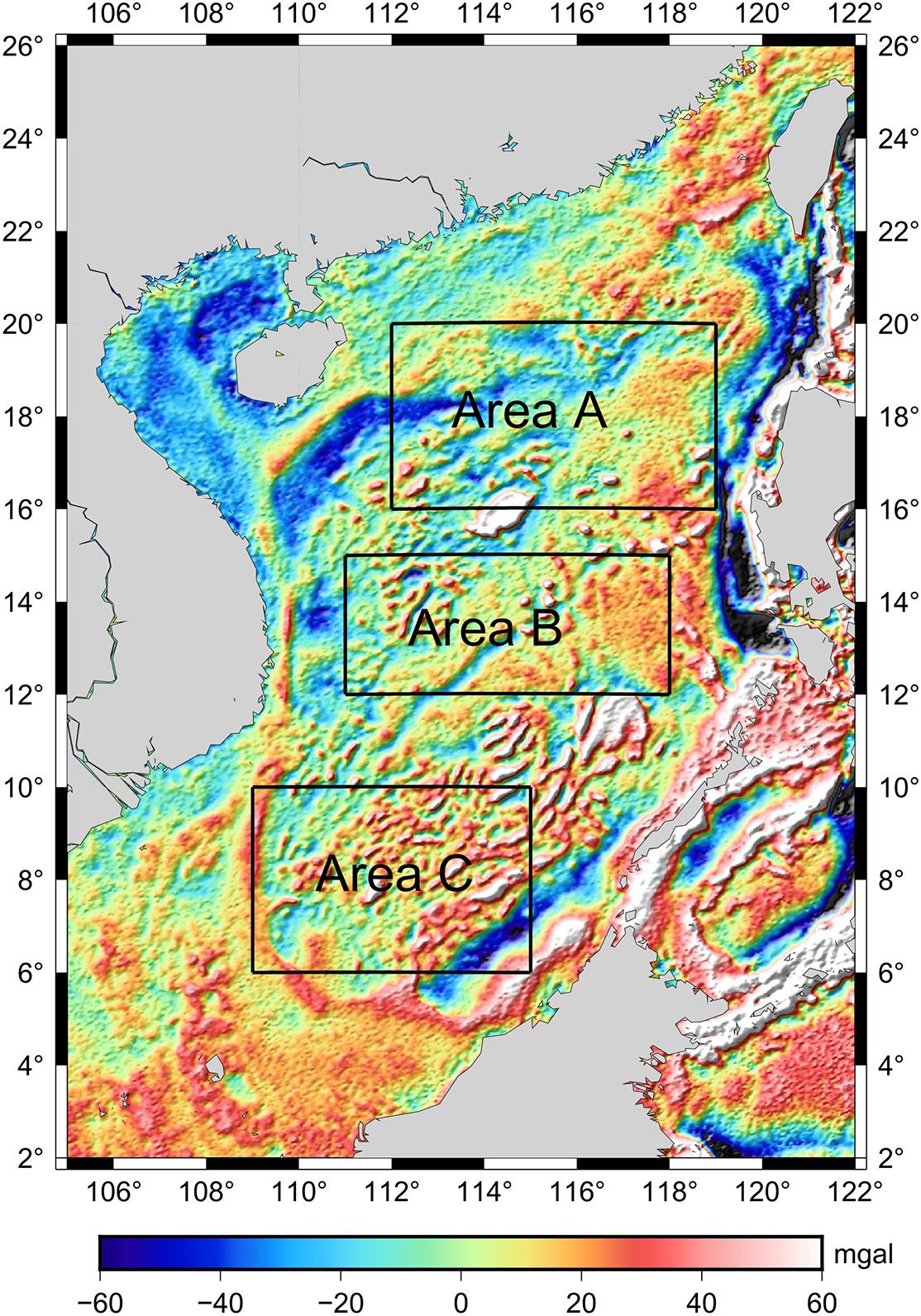
Figure 3. HY-2A/GM-derived 1 arc min gravity anomalies map in the SCS.

Ship-Borne Bathymetry

The ship-borne bathymetry is provided by the National Centers for Environmental Information (NCEI) from the National Oceanic and Atmospheric Administration of the United States (NOAA,¹). The time span of the data is from 1960 to 2016. NCEI controls data quality and gathers qualified data into a database. Although the overall data quality is accurate and reliable, some data have large measurement errors in the early stage, and it is necessary to find these errors. After eliminating ship-borne bathymetry errors, there are 24,386 control points and 12,192 check points in Area A, 27,693 control points and 13,846 check points in Area B, and 9,463 control points and 4,731 check points in Area C. The ratio of control points and check points is 2:1 in each test area. Figure 4 shows the distribution of control points and check points for the test areas.

FIGURE 4

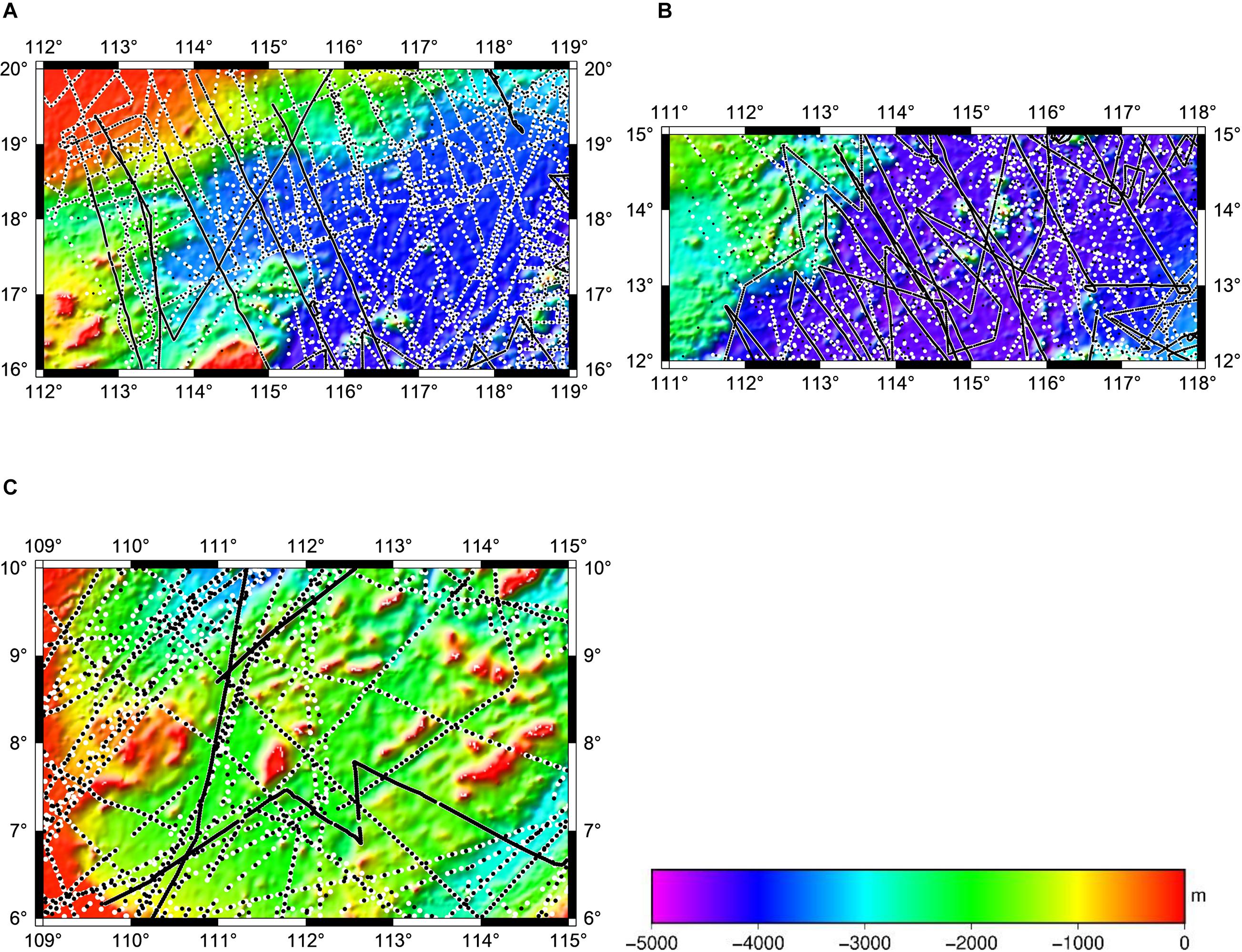
Figure 4. Distribution of ship-borne bathymetry tracks for the test areas of the SCS. (A) Ship-borne bathymetry tracks in test area A. (B) Ship-borne bathymetry tracks in test area B. (C) Ship-borne bathymetry tracks in test area C. By considering the similarity of tomograms, the density of ship track data in each of these regions is evaluated through digital image processing-based metrics. Control points are represented by black points, and check points are represented by white points.

SRTM15+V2.0 Model and GEBCO 2020 Model

Ship-borne bathymetry data has high-precision but does not give uniform coverage, and satellite altimetry data can act as an interpolation to extend bathymetry information beyond ship tracks to the entire chosen region. Satellite altimetry technology improves the resolution and efficiency of various depth models which are built on the basis of ship-borne bathymetry data.

SRTM15+V2.0 model is a global bathymetry and topography grid, and its interval is 15 s. The model is produced by combining ship-borne bathymetry and depth predicted with altimeter-derived gravity. The multibeam and singlebeam measurements data are provided by several institutions, which are Scripps Institution of Oceanography (SIO), the National Geospatial-Intelligence Agency (NGA), Japan Agency for Marine-Earth Science and Technology (JAMSTEC), Center for Coastal and Ocean Mapping (CCOM) and Geoscience Australia (GA). The uncertainty of depth estimation is between −150 and 150 m in the deep ocean (Tozer et al., 2019). In the experiment, for the convenience of comparison, we abbreviated it as SRTM15 model. SRTM15 model can be downloaded from the website: https://figshare.com/articles/online_resource/Tozer_et_al_2019_SRTM15_GMT_Grids/7979780.

The GEBCO 2020 model is a global bathymetry and topography grid, and its interval is 15 s. which is released by the General Bathymetric Chart of the Oceans (GEBCO). the model is built based on SRTM15+V2.0 (Tozer et al., 2019). The data is fused by prediction seabed topography and land topography (GEBCO Bathymetric Compilation Group 2020,2020). In the experiment, for the convenience of comparison, we abbreviated it as GEBCO model. GEBCO model can be downloaded from the website: https://www.gebco.net/data_and_products/gridded_bathymetry_data/gebco_2020/.

Determining the Density Contrast

To make GGM bathymetry values closer to real values, it is necessary to accurately estimate the density contrast of the SCS. First, GGM bathymetry is calculated through the control points under different density contrasts. Then, the depths of check points are obtained with interpolation. Finally, the correlation coefficient and the standard deviation (STD) are obtained by comparing GGM bathymetry with the ship-borne bathymetry. The density contrast is obtained, and gravity anomalies are used to predict bathymetry with GGM (Figure 1).

The reference depths of the test areas are 4,756, 4,903, and 3,921 m by the deepest depth value through control points, respectively. When the correlation coefficient and the standard deviation have extreme points under the same density contrast, the density contrast is appropriate. Based on this principle, with the increase in density contrast, outliers appear in correlation coefficients and standard deviations of the test areas. The density contrasts of the test areas are 1.4, 1.5, and 1.6 g/cm³, respectively; correlation coefficients are 0.999, 0.993, and 0.998, and standard deviations are 53.8, 64.0, and 49.3 m, respectively. Figure 5 shows the trend of correlation coefficients and standard deviations with the density contrast, in the test areas.

FIGURE 5

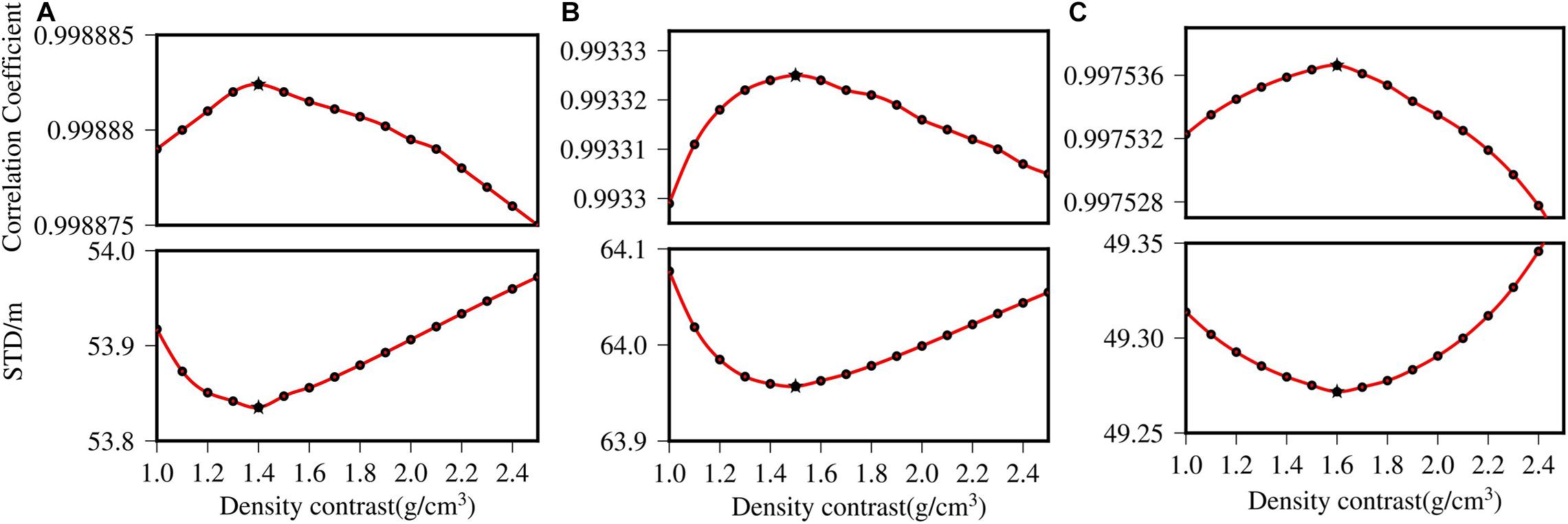
Figure 5. Outliers diagrams for determining density contrast. (A) Determination of Δρ in test area A. (B) Determination of Δρ in test area B. (C) Determination of Δρ in test area C. The variation of correlation coefficient and standard deviation with Δρ in the test areas, and the extreme points are represented by pentagrams. Finally, it is determined that Δρ is 1.4, 1.5, and 1.6 g/cm³ in each of the test areas.

Results and Analysis

Statistics of ship-borne bathymetry, GGM bathymetry, GEBCO model and SRTM15 model at the check points are listed in Table 1. Based on ship-borne bathymetry, the mean depths of the test areas are that A is less than B and greater than C. It can be seen from the mean depths that GGM data are closest to NCEI data in the test areas, while GEBCO data are closest to SRTM15 data in various statistical indicators.

TABLE 1

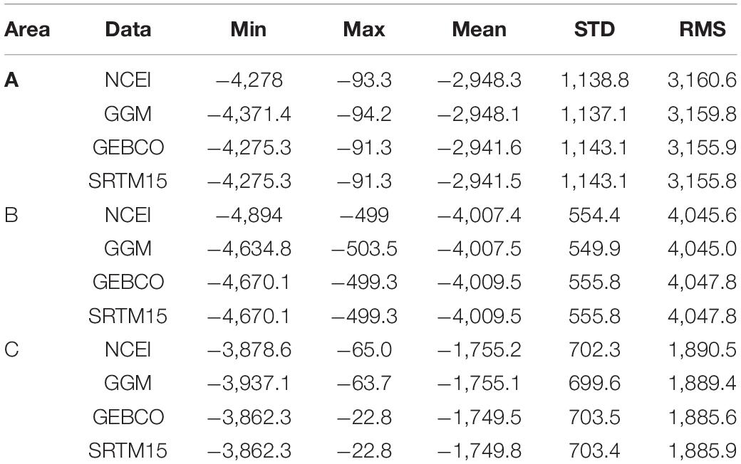
Table 1. Statistics of NCEI ship-borne bathymetry, the GGM bathymetry, GEBCO model, and SRTM15 model in the test areas (unit: m).

Table 2 denotes bathymetry differences between the GGM, NCEI, GEBCO and SRTM15 data, and the results of statistical accuracy at check points. The standard deviations of NCEI-GGM data are 53.8, 64.0, and 49.3 m at the check points, and these mean values of NCEI-GGM data are not more than 0.2 m. The standard deviations of GEBCO-SRTM15 data are 4.5, 3.9, and 16.2 m, respectively, which are smaller than other standard deviations, and the two data have similarity in the statistical data at the check points.

TABLE 2

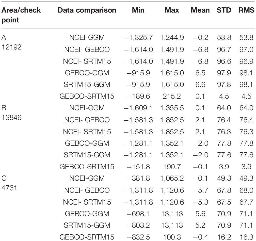
Table 2. Statistics of differences among the NCEI bathymetry, the GGM bathymetry, GEBCO model and SRTM15 model in the check points (unit: m).

Table 3 shows the difference of NCEI-GGM with depth in the test areas. The calculation equation of relative accuracy is as follows:

$$Relativeaccuracy=\frac{1}{\text{n}}\sum _{i=1}^n\left|1-\frac{|H_i-h_i|}{H_i}\right|*100\%(6)$$

TABLE 3

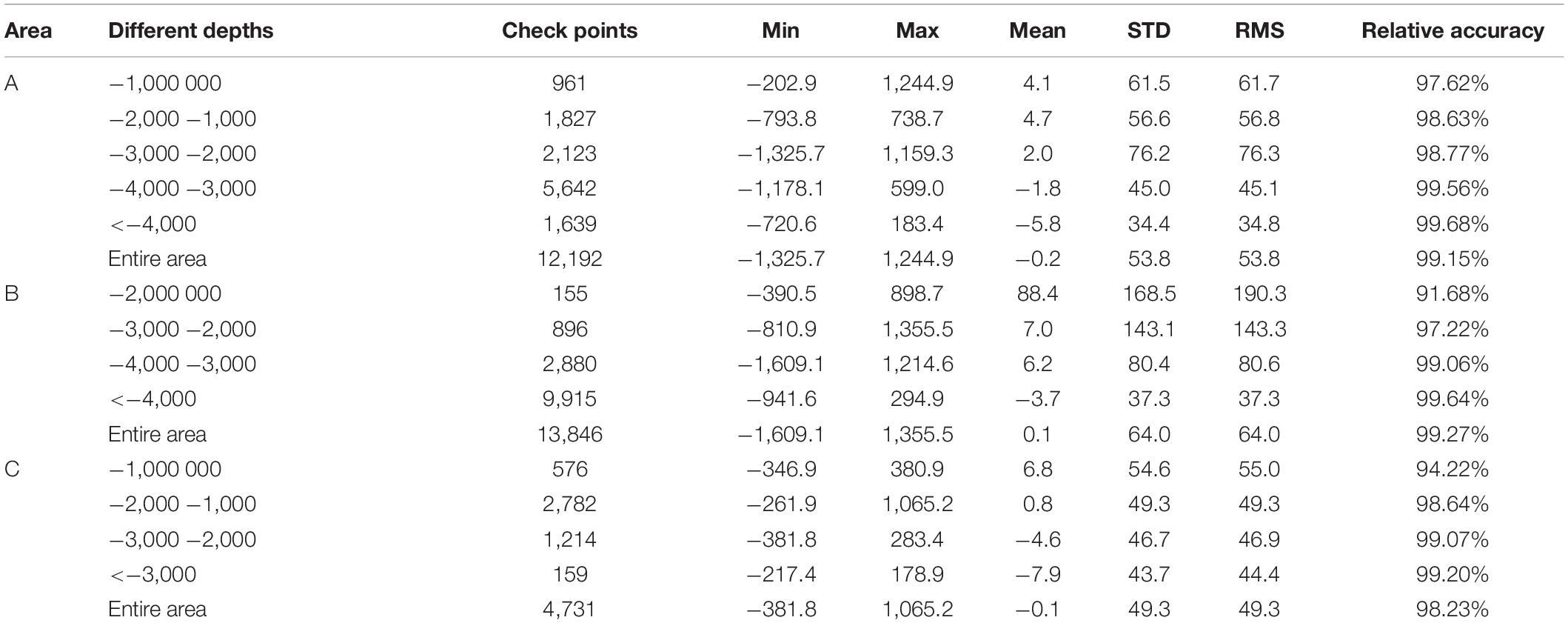
Table 3. Statistics of different depths between the NCEI bathymetry and the GGM bathymetry in the check points (unit: m).

Where H_i denotes ship-borne bathymetry, h_i means the depth calculated by GGMs, n is number of ship-borne points. The results denote that the relative accuracy improves with the increase of depth value in each test area. With the increase of depth, the STD and RMS of each area tend to decrease except for area A ranging from −3,000 to −2,000 m (STD is 56.6 m and RMS is 56.8 m).

Figure 6 presents the histogram of the difference between NCEI and GGM-derived bathymetry predictions. The percentage of error points decreases from the middle to both sides. Table 4 shows the statistical results of error in different ranges, and the errors of GGM bathymetry are concentrated within 50 m data, accounting for 91.65, 87.73, and 87.95% respectively.

FIGURE 6

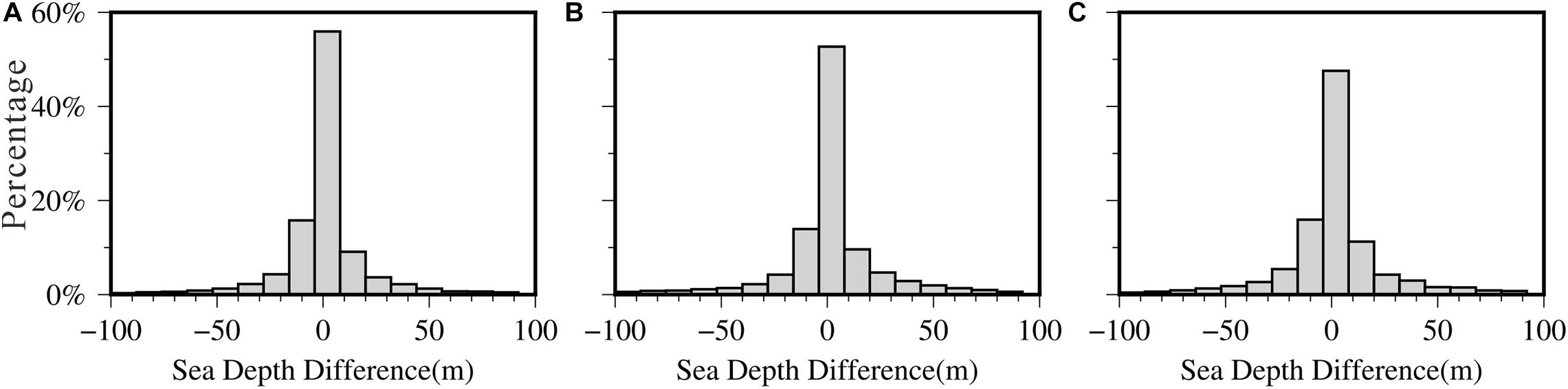
Figure 6. Histograms of the differences between NCEI bathymetry and GGM-derived bathymetry in the check points. (A) Error statistics of test area A. (B) Error statistics of test area B. (C) Error statistics of test area C.

TABLE 4

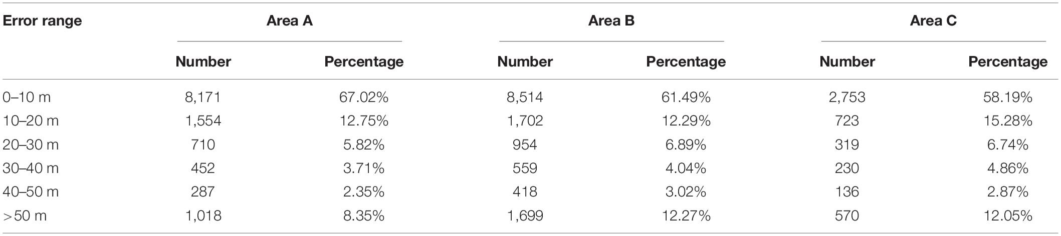
Table 4. Statistics of GGM error range in the check points.

Figure 7 shows the positions of the points where the error is greater than 250 m (black points) at the check points. In Figure 7A, the rectangular I (112.7–116.5°E, 16–18.5°N) has poor accuracy. In Figure 7B, rectangular II (111.85–113.8°E, 13.2–15°N) is the area where the error distribution is concentrated. Rectangular III (113.9–116.6°E, 12.7–15°N) shows that bathymetry of GGM prediction is poor in the area of chain seamounts and linear seamounts. The complex geological structure with great change lead to more error points in these areas. The error points shown in Figure 7C are relatively dispersed, and its error is relatively small.

FIGURE 7

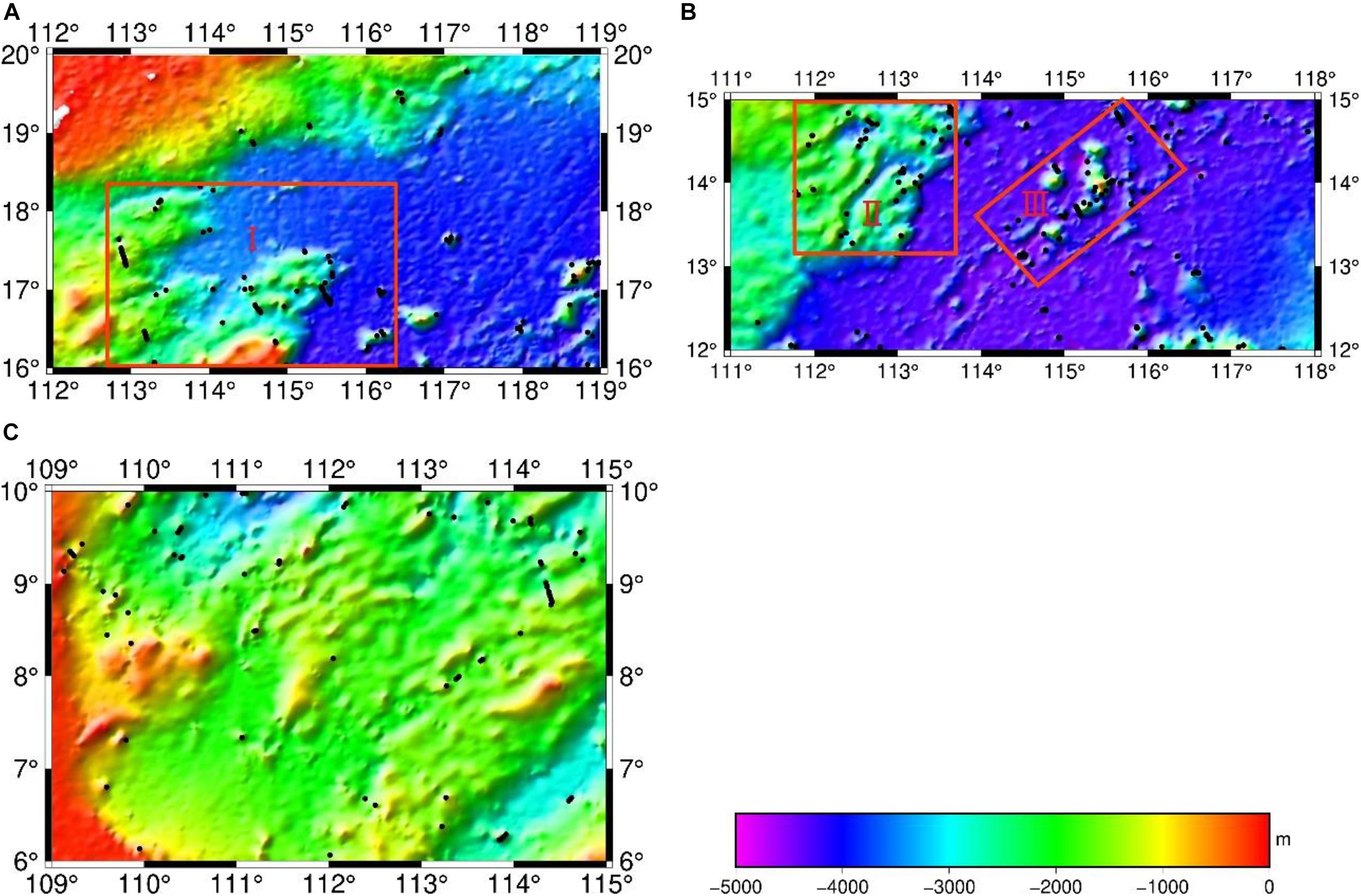
Figure 7. Distribution of differences between NCEI bathymetry and GGM bathymetry in the test areas. (A) Error points distributionin test area A. (B) Error points distributionin test area B. (C) Error points distributionin test area C. The black spot represents the distribution of depth errors greater than 250 m. the red rectangles represents the area with large error, and the background map is GGM bathymetry prediction.

Based on the geological structures of the SCS (Qiu et al., 2016) and GGM bathymetry result (Figure 7), the shape of the SCS basin is an irregular rhombus, and the terrain inclines from the periphery to the center. From the periphery to the center, the large landform units are continental shelf, continental slope and marginal sea basin in the SCS. The terrain of the continental shelf and abyssal basin is relatively gentle, and the terrain of the continental slope is steep. The topography of the continental slope and island slope are rugged, making it the most complex area in the SCS. In this terrain, the accuracy of GGM bathymetry is poor, and its bathymetry accuracy needs to be improved. The abyssal plain is dominated by plain landforms, generally speaking, its terrain is relatively flat, and the accuracy of GGM bathymetry is relatively high. However, when there are chain seamounts and linear seamounts (Figure 7B, rectangular II), the accuracy of GGM bathymetry is relatively poor. The test area C is the southern part of the SCS. Its topography fluctuates little and changes gently. The mean depth is approximately −1,755 m (Table 1), and STD of NCEI-GGM data can reach 49.3m (Table 2) in area C. Through the above analysis, different topography also has an impact on GGM bathymetry. The accuracy of GGM bathymetry is relatively poor in areas with large terrain change, while in areas with gentle change, the accuracy is relatively high.

Some other factors affect the accuracy of GGM bathymetry. The gravity anomalies affect the accuracy of GGM bathymetry. We compare HY-2A/GM-derived gravity anomalies with Sandwell model (it is V29.1 gravity anomalies and is released by Scripps Institution of Oceanography), and the statistical results are shown in Table 5. In test areas, Mean, STD and RMS of GGM_Sandwell and GGM_HY–2A are very close to each other by comparing with NCEI data, and the accuracy of GGM_Sandwell is slightly higher than that of GGM_HY–2A, which is acceptable. Because Sandwell model combines multiple satellite altimetry data, so it is better than HY-2A/GM-derived gravity anomalies in accuracy. The comparison results in Table 5 indicate that it is feasible to use HY-2A/GM-derived gravity to predict bathymetry with GGM, and the gravity anomaly data of HY-2A/GM-derived gravity anomalies are reliable. The interpolation method used to calculate depth with GGM can affect bathymetry accuracy. The comparison results of bathymetry calculated with bilinear interpolation and cubic spline interpolation are shown in Table 6. The results of the cubic spline interpolation used in this paper are better than bilinear interpolation. The accuracy of GGM bathymetry is directly affected with interpolation method, which cannot be neglected.

TABLE 5

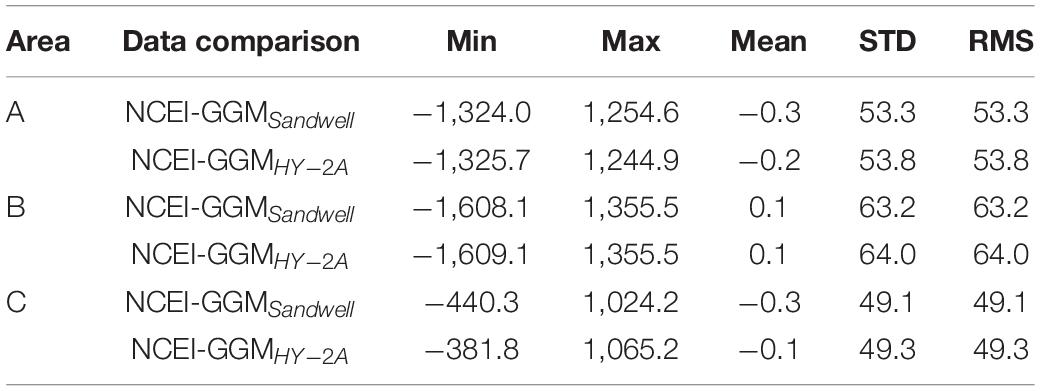
Table 5. Statistics of differences among NCEI data, GGM_Sandwell data, and GGM_HY–2A data in the check points (unit: m).

TABLE 6

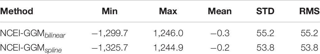
Table 6. Statistics results of difference between NCEI data and bathymetry calculated by bilinear interpolation and cubic spline interpolation in area A (unit: m).

Conclusion

It is feasible to apply HY-2A/GM-derived marine gravity anomalies to predict bathymetry with GGM in the South China Sea. The density contrasts are determined with the iterative method, which improve the accuracy of GGM bathymetry prediction. The comparison with other depth data illustrates that GGM bathymetry is closer to ship-borne bathymetry than those of SRTM15 model and GEBCO model. Moreover, GGM can be applied to areas with sparse ship-borne bathymetry.

The accuracy of GGM bathymetry is analyzed under different geological structures. The accuracy is high in flat terrain, but reduces in complex terrains.

Other factors affecting the accuracy of GGM bathymetry are discussed. Within a certain depth range, as the depth increases, the relative accuracy of GGM bathymetry tends to improve. Based on the ship-borne bathymetry, bathymetry obtained HY-2A/GM-derived gravity anomalies and Sandwell model are compared, and it is concluded that the accuracy of gravity anomalies is also one of the factors affecting bathymetry prediction. In addition, the interpolation method has influence on the result of GGM bathymetry.

If gravity anomalies derived from various satellites and ship-borne are combined to establish a comprehensive gravity field model in the SCS, GGM bathymetry accuracy may be improved. In addition, if GGM bathymetry and other models are assigned different weights, a comprehensive terrain model can be established in the SCS, which may be helpful for the study of geological structure and marine resources.

Data Availability Statement

The raw data supporting the conclusions of this article will be made available by the authors, without undue reservation.

Author Contributions

ZW: scientific analysis and manuscript writing. JG: data quality control. CZ and JY: scientific analysis. XC and BJ: data collection. All authors contributed to the article and approved the submitted version.

Funding

This study is supported by the National Natural Science Foundation of China (grant Nos. 41774001, 41374009, 41774021, and 41874091), and the SDUST Research Fund (grant No. 2014TDJH101).

Conflict of Interest

The authors declare that the research was conducted in the absence of any commercial or financial relationships that could be construed as a potential conflict of interest.

Acknowledgments

We would like to thank NCEI for providing the ship-borne bathymetry data. We would also like to thank Cheinway Hwang and Yu-Shen Hsiao.

Footnotes

1. ^ http://www.noaa.gov

References

Adams, J. M., and Hinze, W. J. (1990). The gravity-geologic technique of mapping buried bedrock topography. Geotech. Environ. Geophys. 3, 99–106. doi: 10.1190/1.9781560802785.3

CrossRef Full Text | Google Scholar

Born, G. H., Dunne, J. A., and Lame, D. B. (1979). Seasat mission overview. Science 204, 1405–1406. doi: 10.1126/science.204.4400.1405

PubMed Abstract | CrossRef Full Text | Google Scholar

Calmant, S., and Baudry, N. (1996). Modelling bathymetry by inverting satellite altimetry data: a review. Mainer Geophys. Res. 18, 123–135. doi: 10.1007/BF00286073

CrossRef Full Text | Google Scholar

Centre National d’Etudes Spatiales (CNES) (2017). Along-track level-2+ (L2P) SLA product handbook.SALP-MU-P-EA-23150-CLS, Issue 1.0. Available online at: https://www.aviso.altimetry.fr/fileadmin/documents/data/tools/hdbk_L2P_all_missions_except_S3.pdf (accessed October 11, 2019)

Google Scholar

Cheney, R., Douglas, B., Green, R., Miller, L., Milbert, D., and Porter, D. (1986). The GEOSAT altimeter mission: a milestone in satellite oceanography. EOS Trans. Am. Geophys. Union 67, 1354–1355. doi: 10.1029/EO067i048p01354

CrossRef Full Text | Google Scholar

Coiras, E., Petillot, Y., and David, M. L. (2007). Multiresolution 3-D reconstruction from side-scan sonar images. IEEE Trans. Image Process. 16, 382–390. doi: 10.1109/TIP.2006.888337

PubMed Abstract | CrossRef Full Text | Google Scholar

Dorman, L. M., and Lewis, B. T. R. (1970). Experimental isostasy: 1. theory of the determination of the earth’s isostatic response to a concentrated load. J. Geophys. Res. 75, 3357–3365. doi: 10.1029/JB075i017p03357

CrossRef Full Text | Google Scholar

Francis, C. R., Graf, G., Edwards, P. G., McCraig, M., McCarthy, C., Lefebvre, A., et al. (1995). The ERS-2 spacecraft and its payload. Eur. Space Agency Bull. 83, 13–31.

Google Scholar

GEBCO Bathymetric Compilation Group 2020 (2020). The GEBCO_2020 Grid–A Continuous Terrain Model of the Global Oceans and Land. Liverpool: British Oceanographic Data Centre, National Oceanography Centre, NERC, doi: 10.5285/a29c5465-b138-234d-e053-6c86abc040b9

PubMed Abstract | CrossRef Full Text | Google Scholar

Grant, F. S., and West, G. F. (1965). Interpretation Theory In Applied Geophysics. New York, NY: McGraw-Hill Book.

Google Scholar

Guo, J., Gao, Y., Hwang, C., and Sun, J. (2010). A multi-subwaveform parametric retracker of the radar satellite altimetric waveform and recovery of gravity anomalies over coastal oceans. Sci. China Earth Sci. 53, 610–616. doi: 10.1007/s11430-009-0171-3

CrossRef Full Text | Google Scholar

Guo, J., Liu, X., Chen, Y., Wang, J., and Li, C. (2014). Local normal height connection across sea with ship-borne gravimetry and GNSS techniques. Mar. Geophys. Res. 35, 141–148. doi: 10.1007/s11001-014-9216-x

CrossRef Full Text | Google Scholar

Guo, J., Shen, Y., Zhang, K., Liu, X., Kong, Q., and Xie, F. (2016). Temporal-spatial distribution of oceanic vertical deflections determined by TOPEX/Poseidon and Jason-1/2 missions. Earth Sci. Res. J. 20, 1–5. doi: 10.15446/esrj.v20n2.54402

CrossRef Full Text | Google Scholar

Guo, J. Y., Wang, J. B., Hu, Z. B., Hwang, C. W., Chen, C. F., and Gao, Y. G. (2015). Temporal-spatial variations of sea level over China seas derived from altimeter data of TOPEX/Poseidon, Jason-1 and Jason-2 from 1993 to 2012. Chin. J. Geophys. 58, 3103–3120. doi: 10.6038/cjg20150908

CrossRef Full Text | Google Scholar

Hsiao, Y. S., Hwang, C., Cheng, Y., Chen, L., Hsu, H., Tsai, J., et al. (2016). High-resolution depth and coastline over major atolls of South China Sea from satellite altimetry and imagery. Remote Sens. Environ. 176, 69–83. doi: 10.1016/j.rse.2016.01.016

CrossRef Full Text | Google Scholar

Hsiao, Y. S., Kim, J. W., Kim, K. B., Lee, B. Y., and Hwang, C. (2011). Bathymetry estimation using the gravity-geologic method: an investigation of density contrast predicted by the downward continuation method. Terr. Atmos. Ocean. Sci. 22, 347–358. doi: 10.3319/TAO.2010.10.13.01

CrossRef Full Text | Google Scholar

Hu, M. Z., Li, J. C., and Jin, T. Y. (2012). Bathymetry inversion with gravity-geological gethod in emperor seamount. Geomatics Inform. Sci. Wuhan Univ. 37, 610–612. doi: 10.13203/j.whugis2012.05.008

CrossRef Full Text | Google Scholar

Hwang, C. (1999). A bathymetry model for the South China Sea from satellite altimetry and depth data. Mar. Geod. 22, 37–51. doi: 10.1080/014904199273597

CrossRef Full Text | Google Scholar

Hwang, C., Guo, J., Deng, X., Hsu, H. Y., and Liu, Y. (2006). Coastal gravity anomaly from retracked Geosat/GM altimetry: improvement, limitation and the role of airborne gravity data. J. Geod. 80, 204–216. doi: 10.1007/s00190-006-0052-x

CrossRef Full Text | Google Scholar

Hwang, C., Hsu, H. J., Chang, E. T. Y., Featherstone, W. E., Tenzer, R., Lien, T., et al. (2014). New free-air and Bouguer gravity fields of Taiwan from multiple platforms and sensors. Tectonophysics 611, 83–93. doi: 10.1016/j.tecto.2013.11.027

CrossRef Full Text | Google Scholar

Hwang, C., Hsu, H. Y., and Jang, R. J. (2002). Global mean sea surface and marine gravity anomaly from multi-satellite altimetry: applications of deflection-geoidand inverse Vening Meinesz formulae. J. Geod. 76, 407–418. doi: 10.1007/s00190-002-0265-6

CrossRef Full Text | Google Scholar

Ibrahim, A., and Hinze, W. J. (1972). Mapping buried bedrock topography with gravity. Ground Water 10, 18–23. doi: 10.1111/j.1745-6584.1972.tb02921.x

CrossRef Full Text | Google Scholar

Jay, S., and Guillaume, M. (2014). A novel maximum likelihood based method for mapping depth and water quality from hyperspectral remote-sensing data. Remote Sens. Environ. 147, 121–132. doi: 10.1016/j.rse.2014.01.026

CrossRef Full Text | Google Scholar

Kim, J. W., Frese, R. R. B., Frese, V., Lee, B. Y., Roman, D. R., and Doh, S. J. (2011). Altimetry-derived gravity predictions of bathymetry by the gravity-geologic method. Pure Appl. Geophys. 168, 815–826. doi: 10.1007/s00024-010-0170-5

CrossRef Full Text | Google Scholar

Kim, K. B., Hsiao, Y. S., Kim, J. W., Lee, B. Y., Kwon, Y. K., and Kim, C. H. (2010). Bathymetry enhancement by altimetry-derived gravity anomalies in the East Sea (Sea of Japan). Mar. Geophys. Res. 31, 285–298. doi: 10.1007/s11001-010-9110-0

CrossRef Full Text | Google Scholar

Li, Z., Liu, X., Guo, J., Zhu, C., Yuan, J., Gao, J., et al. (2020). Performance of Jason-2/GM altimeter in deriving marine gravity with the waveform derivative retracking method: a case study in the South China Sea. Arab. J. Geosci. 13:939. doi: 10.1007/s12517-020-05960-0

CrossRef Full Text | Google Scholar

Luo, J., Li, J. C., and Jiang, W. P. (2002). Bathymetry prediction of South China Sea from satellite data. Geomatics Inform. Sci. Wuhan Univ. 27, 256–260. doi: 10.13203/j.whugis2002.03.006

CrossRef Full Text | Google Scholar

Ouyang, M. D., Sun, Z. M., and Zhai, Z. H. (2014). Predicting bathymetry in South China Sea using the gravity-geologic method. Chin. J. Geophys. 57, 2756–2765. doi: 10.6038/cjg20140903

CrossRef Full Text | Google Scholar

Qiu, Y., Wang, J., Yan, P., Huang, W. K., Zhu, B. D., and Wang, Y. L. (2016). Characteristics of the crustal structure in the South China Sea and their tectonic significance. Geol. Study S. China Sea 1, 1–39.

Google Scholar

Sandwell, D. T., and Smith, W. H. F. (1997). Marine gravity anomaly from Geosat and ERS-1 satellite altimetry. J. Geophys. Res. 102, 10039–10054. doi: 10.1029/96JB03223

CrossRef Full Text | Google Scholar

Sandwell, D. T., and Smith, W. H. F. (2009). Global marine gravity from retracked Geosat and ERS-1 altimetry: ridge segmentation versus spreading rate. J. Geophys. Res. 114:B01411. doi: 10.1029/2008JB006008

CrossRef Full Text | Google Scholar

Silva, J. B., Costa, D. C., and Barbosa, V. C. (2006). Gravity inversion of basement relief and estimation of density contrast variation with depth. Geophysics 71, 51–58. doi: 10.1190/1.2236383

CrossRef Full Text | Google Scholar

Smith, W. H. F., and Sandwell, D. T. (1994). Bathymetry prediction from dense satellite altimetry and sparse ship-borne bathymetry. J. Geophys. Res. 99, 21803–21824. doi: 10.1029/94JB00988

CrossRef Full Text | Google Scholar

Tozer, B., Sandwell, D. T., Smith, W. H. F., Olson, C., Beale, J. R., and Wessel, P. (2019). Global bathymetry and topography at 15 arc sec: SRTM15+. Earth Space Sci. 6, 1847–1864. doi: 10.1029/2019ea000658

CrossRef Full Text | Google Scholar

Watts, A. B. (1978). An analysis of isostasy in the world’s oceans 1: Hawaiian-Emperor seamount chain. J. Geophys. Res. 83, 5989–6004. doi: 10.1029/JB083iB12p05989

CrossRef Full Text | Google Scholar

Zhu, C., Guo, J., Gao, J., Liu, X., Hwang, C., Yu, S., et al. (2020). Marine gravity determined from multi-satellite-GM/ERM altimeter data over the South China Sea: SCSGA V1.0. J. Geod. 94:50. doi: 10.1007/s00190-020-01378-4

CrossRef Full Text | Google Scholar

Zhu, C., Guo, J., Hwang, C., Gao, J., Yuan, J., and Liu, X. (2019). How HY-2A/GM altimeter performs in marine gravity derivation: assessment in the South China Sea. Geophys. J. Int. 219, 1056–1064. doi: 10.1093/gji/ggz330

CrossRef Full Text | Google Scholar