Correlation Analysis of Influencing Factors and the Monthly Displacement Increment of a Hydrodynamic Landslide Using a Pseudo-Maximum-Likelihood-Estimation-Mixed-Copula Approach

Introduction

The Three Gorges Hydropower Station is currently the largest hydropower station in the world, and it is the largest project ever constructed in China. Since the start of the experimental water storage in 2003, it has been in continuous operation for 16 years. Because of the complex geological conditions and the frequent human activities in TGRA, this area has been prone to frequent geological disasters over a long period of time (Chen et al., 2008; Yin et al., 2009; Kirschbaum et al., 2010; Miyagi et al., 2011; Ahmed, 2015). The ecological environment of the reservoir has deteriorated as a result of landslides caused by heavy rainfall and reservoir water-level changes, which has become a major potential hazard affecting the long-term operational safety of major hydropower projects and the ecological environment of the reservoir (Varnes, 1996). Important topics in the field of hydrodynamic landslide disaster monitoring and early warning and prevention include: 1) the analysis of the reservoir’s hydrodynamic landslide deformation characteristics and the deformation-induced response, 2) the analysis of landslide influencing factors and deformation prediction, and 3) the establishment of a threshold extraction model. To reveal the disaster-causing mechanism of hydrodynamic landslides in reservoir areas, it is particularly important to study the correlation between the influencing factors and the displacement, which holds great significance for the monitoring and early warning of reservoir disasters and the prevention and mitigation of geological disasters.

Currently, correlation analysis of influencing factors of landslide deformation has been based primarily on linear theory. For instance, some traditional correlation analysis methods, such as linear correlation analysis, gray correlation analysis, and hypothesis testing, have been applied to select the influencing factors that affect the displacement of the hydrodynamic landslide (Ohtake, 1986; Kafri and Shapira, 1990; Wang et al., 2004; Pavan et al., 2012; Telesca et al., 2012; Miao et al., 2017a). In addition, some researchers have used autoregressive–moving-average (ARMA) time series analysis and Pearson product-moment correlation coefficients (PPCC) to analyze the lagged correlation between the monthly displacement increments and their influencing factors (Cai et al., 2016; Cao et al., 2016; Zhou et al., 2016; Li et al., 2018). Moreover, based on the daily rainfall data for the TGRA, the finite element method (FEM) and discrete element method (DEM) also have been used to simulate the effect of influencing factors on landslide stability and have verified the correlation between influencing factors and landslide displacement (Kawamoto, 2005; Lollino et al., 2010; Tang et al., 2017). Data-mining technique and clustering method have been applied to interpret landslide monitoring data and to select the influencing factors of the landslide deformation (Shiuan, 2012; Hong et al., 2016; Ma et al., 2016).

These research models and methods based on linear theory, however, can just depict the linear relationship between two variables, and they ignore the thick-tailed variables. Thus, they cannot satisfactorily represent the full relationship between the two variables, and it becomes extremely difficult to accurately measure the correlation structure of the two random variables when the distribution function of the random variables is uncertain or too complex (Iyengar, 1997).

Because the influences associated with landslide hazards are uncertain and dynamic (Bai et al., 2010), a more flexible and robust nonlinear correlation analysis tool (i.e., the Copula theory; (Sklar, 1959) has been used to analyze the correlation structure between variables when it is not certain that linear correlation coefficients can properly measure the correlation. In addition, the Copula method offers many advantages over traditional correlation analysis methods (Sklar, 1959).

Thus, the Copula model often is used to construct complex multidimensional probability distributions. For example, several kinds of Copula models were used to generate the joint probability density distributions of the rainfall, reservoir water-level changes, and landslide displacement to study their tail correlation (Motamedi and Liang, 2014; Bezak et al., 2016; Miao et al., 2017; Li et al., 2018; Wang et al., 2020). These methods, however, still have limitations (Hu, 2002). The Copula functions that belong to the elliptic Copula family in the high-dimensional construction case are extremely difficult, whereas construction of the Archimedean Copula function is simple. When the correlation between the random variables is too complex, using a single Archimedean or elliptic Copula function is more likely to produce a one-sided description. To solve this problem, the M-Copula method combing Frank, Clayton, and Gumbel Copula functions has been used for relationships and risk analysis between two random variables (Liu and Zhang, 2016). More important, nearly all of these methods have used the full maximum likelihood estimation (MLE) method to estimate the parameters of the Copula model. The MLE method, however, requires prior assumption of the marginal distribution of the random variables, which directly affects the results of the parameter estimation if the marginal distribution is incorrectly selected.

In summary, we proposed a new pseudo-MLE-M-Copula model to quantitatively investigate the correlation between the displacement of the Bazimen landslide and the influences of the rainfall and reservoir water-level fluctuations in the TGRA. This model not only overcomes the shortcomings of the linear method and more accurately describes the joint distribution relationship between the random variables, but also linearly combines the Gumbel Copula, Frank Copula, and Clayton Copula functions in the Archimedean Copula family to construct the M-copula function model. This model is more comprehensive and flexible, allowing it to describe complex correlations, and also adopts a semi-parametric estimation method. Thus, the pseudo-MLE, for the parameter estimation of the Copula model, eliminates the need to assume the marginal distributions and can effectively reduce the error of the parameter estimation. This research has provided the scientific basis for the study of reservoir hydrodynamic landslide disaster-causing mechanisms, landslide disaster monitoring and early warning, and disaster prevention and mitigation.

Methodology

Copula Theory

Copula functions generally include two classes (Reboredo, 2011): the Archimedean Copula and the elliptical Copula. The elliptical Copula includes the normal Copula function and the t-Copula function, whereas the Archimedean Copula family includes the Gumbel-Hougaard function, the Clayton function, and the Frank function. (Mackay, 1986; Nelsen, 1986). The Archimedean Copula function family has been used widely because of the simplicity of its computation process and the relative clarity of the construction model as well as because it is not limited by the positive or negative correlations between the different variables (Yan, 2006). Given random variables x and y, the two-dimensional Archimedean Copula function is defined as follows:

$C\left(u_1,u_2\right)={\phi }^{-1}\left[\phi \left(u_1\right),\phi \left(u_2\right)\right], \hspace{1em}0<u_1<u_2<1,(1)$

where $\phi \left(u\right)$ and ${\phi }^{-1}\left(u\right)$ are the element generators and their inverse functions for the Archimedean Copula, respectively; $u_1$ is the marginal distribution of variable x; and $u_2$ is the marginal distribution of variable y. The Gumbel, Clayton, and Frank Copula functions used in this study are shown below, respectively:

$C_1\left(u_1,u_2\right)=\exp \left\{-{\left[-{\left(\log u_1\right)}^{{\beta }_1}+{\left(-\log u_2\right)}^{{\beta }_1}\right]}^{\left(1/{\beta }_1\right)}\right\},\hspace{1em}{\beta }_1\ge 1,(2)$

$C_2\left(u_1,u_2\right)={\left(u_1^{-{\beta }_2}+u_2^{-{\beta }_2}-1\right)}^{-\left(1/{\beta }_2\right)},\hspace{1em} 0<{\beta }_2<\infty ,(3)$

$C_3\left(u_1,u_2\right)=\frac{1}{{\beta }_3}\log \left(1+\frac{\left(e^{{\beta }_3{u}_1}-1\right)\left(e^{{\beta }_3{u}_2}-1\right)}{e^{{\beta }_3}-1}\right), \hspace{1em}-\infty <{\beta }_3<\infty .(4)$

In Eqs 2–4, $C_1\left(u_1,u_2\right)$, $C_2\left(u_1,u_2\right)$, and $C_3\left(u_1,u_2\right)$ are the Gumbel, Clayton, and Frank Copula functions, respectively; and α, θ, and γ are their corresponding parameters.

In 2002, Hu proved that if these three Archimedean Copula functions were combined linearly by adding coefficients (Hu, 2002), a mixed Copula function could be formed. The mixed function, which has all of the good features of the three Copula functions, can be described from several different angles to depict the more complex correlations between the variables. The expression is as follows:

$C_M=m_1{C}_1+m_2{C}_2+m_3{C}_3,(5)$

where $C_1$, $C_2$, and $C_3$ are the Gumbel, Clayton, and Frank Copula functions; $m_1$, $m_2$, and $m_3$ are the weighting coefficients of the three Copula functions, respectively; and $m_1$, $m_2$, and $m_3$ are ≥0, and $m_1+m_2+m_3=1$.

The tail correlation coefficient (Zhang and Singh, 2007a) includes the lower-tail correlation coefficient and the upper-tail correlation coefficient. The lower-tail correlation coefficient represents the effect on another random variable when one random variable takes a smaller value and is given by the following formula:

${\lambda }^{lo}=\underset{u\to 1}{\text{lim}}P\left[Y<G^{-1}\left(u\right)|X<F^{-1}\left(u\right)\right]=\underset{u\to 1}{\lim }\frac{\widehat{C}\left(1-u,1-u\right)}{1-u}.(6)$

The upper-tail correlation coefficient represents the effect on another random variable when one variable takes a larger value, and it is given by the following formula:

${\lambda }^{up}=\underset{u\to 0}{\text{lim}}P\left[Y>G^{-1}\left(u\right)|X>F^{-1}\left(u\right)\right]=\underset{u\to 0}{\lim }\frac{C\left(u,u\right)}{u},(7)$

where $u\in \left[\mathrm{0,1}\right]$; and $\widehat{C}=1-2u+C\left(u,u\right)$ is the Copula survival function. If ${\lambda }^{lo}$ and ${\lambda }^{up}$ exist and both are in the interval [0, 1], the larger the value, the stronger the correlation. If ${\lambda }^{lo}$ and ${\lambda }^{up}$ are equal to 0, the random variables in the upper and lower tails are independent of each other.

To further study the influence of each influencing factor on the landslide displacement deformation, we constructed a value-at-risk (VaR) model (Rockafellar and Uryasev, 2002) and tailed value-at-risk (TVaR) based on the Copula parameters and extracted the thresholds. The expression is as follows:

$Va{R}_{\alpha }\left(x\right)={\widehat{F}}^{-1}\left(x\right),(8)$

$TVa{R}_{\alpha }=-\frac{{\displaystyle {\int }_0^{\alpha }Va{R}_r\left(x\right)\text{d}r}}{\alpha }(9)$

where $x$ is the value of each influencing factor; $\alpha$ is the confidence level (0.95 in this study); and ${\widehat{F}}^{-1}\left(x\right)$ is the cumulative probability density function of the selected optimal Copula function.

Building a Correlation Model Based on a Copula Function

Data Preprocessing

To analyze the correlation between the rainfall, the reservoir water-level fluctuations, and the landslide deformation, we selected the optimal Copula model. From the type of data source, we knew that the monthly displacement increment, the rainfall, the two-month rainfall, the one-month reservoir water-level change, and the two-month reservoir water-level change were all discrete data. Thus, a discrete data transformation should be considered when constructing the binary Copula model. In this study, we used the distribution function transformation method proposed by Wu (Wu et al., 2009), which could solve the problem faster. The core idea of this method was that the random variable X (discrete or continuous) was known, and for any real number in x ∈ R, k ∈ I, and the defining functions are as follows:

$D\left(x,k\right)=P\left(X<x\right)+kP\left(X=x\right),(10)$

where k obeys a uniform distribution and is independent of X. From this, the generalized distribution function transformation of X is obtained:

$Q=D\left(x,k\right).(11)$

In this study, we used this method to carry out the generalized transformation of the four impact factor data sets X and the monthly displacement increment data Y:

$Q_x=D\left(x,k\right)=P\left(X<x\right)+kP\left(X=x\right),(12)$

$Q_y=D\left(y,k\right)=P\left(Y<y\right)+kP\left(Y=y\right).(13)$

Parameter Estimation

The process of estimating the parameters of these four Copula functions using the MLE method (Dempster et al., 1977; Liu and Zhang, 2016) is as follows: Assume that the joint distribution of two-dimensional random variables is $H_M$, and the marginal distribution is continuous; they are $F_1,F_2$ respectively. According to Sklar’s theorem,

$H_M\left(m_1,m_2,m_3;{\beta }_1,{\beta }_2,{\beta }_3\right)={\displaystyle \sum _{j=1}^3{m}_j{C}_j\left(F_1,F_2;{\beta }_i\right)},(14)$

where $C_j$ is the Archimedes Copula function family with parameter ${\beta }_j$, and $C_j\left(F_1,F_2;{\beta }_i\right)$ is one single Archimedean Copula model, ${\displaystyle {\sum }_{j=1}^3{m}_j{C}_j\left(F_1,F_2;{\beta }_i\right)}$ is the expression of the M-Copula model. The main difference between MLE and pseudo-MLE is that the marginal distribution will be replaced with the empirical distribution function (Genest, 1987), and the expression of empirical distribution is as follows:

${\widehat{F}}_j\left(x\right)=\frac{1}{n}{\displaystyle {\sum }_{i=1}^n\mathbf{1}\left(X_{ij}\le t\right)}.(15)$

So the joint density function with the empirical distribution is:

$h_M\left(m_1,m_2,m_3;{\beta }_1,{\beta }_2,{\beta }_3\right)=\frac{{\partial }^{2}H}{\partial F_1\partial F_2}={\displaystyle \sum _{j=1}^3{m}_j{c}_j\left({\widehat{F}}_1,{\widehat{F}}_2;{\beta }_j\right)}.(16)$

Sample $\left(F_{1i},F_{2i}\right)\left(i=\mathrm{1,2},\dots ,n\right)$, the likelihood function is:

$L\left(m_1,m_2,m_3;{\beta }_1,{\beta }_2,{\beta }_3\right)={\displaystyle \prod _{i=1}^n\left({\displaystyle \sum _{j=1}^3{m}_j{c}_j\left({\widehat{F}}_{1\text{i}},{\widehat{F}}_{2\text{i}};{\beta }_j\right)}\right)}.(17)$

The log likelihood function is:

$\ln L\left(m_1,m_2,m_3;{\beta }_1,{\beta }_2,{\beta }_3\right)={\displaystyle \sum _{i=1}^n\left({\displaystyle \sum _{j=1}^3{m}_j{c}_j\left({\widehat{F}}_{1i},{\widehat{F}}_{2i};{\beta }_j\right)}\right)}.(18)$

Solving the maximum point of the log-likelihood function, the pseudo-maximum likelihood estimates of $m_j$ and ${\beta }_j$ can be obtained:

${\widehat{m}}_1,{\widehat{m}}_2,{\widehat{m}}_3;{\widehat{\beta }}_1,{\widehat{\beta }}_2,{\widehat{\beta }}_3=\arg \max \ln L\left(m_1,m_2,m_3;{\beta }_1,{\beta }_2,{\beta }_3\right).(19)$

Goodness-of-Fit Test

The pattern of the correlations between the multidimensional random variables can be described by the Copula model. The many types of Copula models reflect the different correlation patterns. To select the most appropriate Copula model for this study, we first selected the optimal model based on the Akaike information criterion (AIC), the Bayesian information criterion (BIC), and the root mean squared error (RMSE) values. Then, we used the Kolmogorov-Smirnov test (K-S test) to determine whether the optimal Copula model reflected the correct correlation structure between the variables.

The AIC is a judgment method based on the measurement of information, and it is suitable for testing the Copula models obtained using the MLE method. The BIC is more sensitive to models that are overestimated.

$AIC=N\log \left[\frac{1}{N}{\displaystyle \sum _{k=1}^N{\left(x_k^{est}-x_k^{emp}\right)}^2}\right]+2n.(20)$

$BIC=N\log \left[\frac{1}{N}{\displaystyle \sum _{k=1}^N{\left(x_k^{est}-x_k^{emp}\right)}^2}\right]+n\log N.(21)$

We used the RMSE to describe the error between the predictive Copula model and the empirical Copula model, as follows:

$RMSE=\sqrt{\frac{{\displaystyle {\sum }_{k=1}^N{\left(x_k^{est}-x_k^{emp}\right)}^2}}{N}},(22)$

where $x_k^{est}$ represents the predicted estimated values, $x_k^{emp}$ represents the empirical values, N is the capacity of the entire sample, and n is the number of parameters in the model.

The K-S test (Christian and Bruno, 2008) can be used to test whether a sample obeys a specified distribution. We constructed the statistics of the K-S test according to the fact that the derivative of the Copula function obeys a uniform distribution within (0, 1). The original assumption $H_0$ was that a partial derivative of the selected Copula model obeys a uniform distribution within (0, 1).

$D_{\max }=\sqrt{n}\text{max}\left\{\left|F_n\left(x_{i-1}\right)-F\left(x_i\right)\right|\left|F_n\left(x_i\right)-F\left(x_i\right)\right|\right\},(23)$

where $F_n\left(x\right)$ is one of the partial derivatives of the Copula function; and $F\left(x\right)$ is a uniform distribution within (0, 1). Given a testing level α and a sample capacity n, the fractional table was used to find the critical value $D_{n,\alpha }$. If $D_{\max }>D_{n,\alpha }$, then $H_0$ is rejected; otherwise, $H_0$ is accepted.

Conditional Probability Distribution and Return Period

We further studied the joint distribution of the two random variables under different influencing factors (Zhang and Singh, 2007b). The conditional probability distribution was calculated using Eq. 23, and the periodic variations in the variables were described using the return period concept, which represents the number of time intervals per occurrence averaged over a certain hydrological variable greater than or equal to a specified value (Eq. 24).

$F\left(y|X=x\right)=C\left(V\le v|U=u\right)=\frac{\partial C\left(u,v\right)}{\partial u}.(24)$

$T\left(y|X=x\right)=\frac{1}{1-F\left(y|X=x\right)}=\frac{1}{1-\left(\partial C\left(u,v\right)/\partial u\right)}.(25)$

Building the Correlation Model

According to the field monitoring curves for the displacement of the Bazimen landslide and the reservoir’s water level and rainfall, we found that the reservoir’s water level, rainfall, and monthly landslide displacement increment exhibited different trends with time. First, the annual cycle of the reservoir water-level fluctuations and the rainfall exhibit a certain periodicity because of the existence of a rainy season in this region. Second, the monthly displacement increment of the reservoir landslide’s deformation exhibited a weak periodicity under the effects of rainfall and reservoir water-level changes. To reveal the influences of the rainfall and reservoir water-level changes on the landslide deformation, in this study, we used the Copula model to assess the correlations between each influencing factor and the incremental monthly displacement of the landslide. The work flow of the correlation analysis of the landslide deformation and the influencing factors based on the Copula model is shown in Figure 1. It has two parts: model selection and model application and correlation analysis.

FIGURE 1

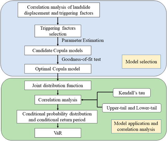
FIGURE 1. Flowchart of this research.

The specific implementation process is as follows. First, we selected the appropriate influencing factors to construct the Copula model, selected the optimal model based on the results of the goodness-of-fit test, established the joint probability density distribution functions for the landslide’s monthly displacement increment and influencing factors, and analyzed the overall and tail correlations between the influencing factors and the landslide’s monthly displacement increment. We constructed the conditional probability distribution model of the M-Copula function, and then calculated the conditional distribution of the displacement increment under different conditions. Accordingly, we obtained the return period of the displacement increment under the corresponding conditions. Finally, we extracted the thresholds of the rainfall and reservoir water-level changes in the reservoir area. This entire process plays an active role in the prevention and mitigation of hydrodynamic landslides in the TGRA.

Case Study: Bazimen Landslide

Data Source and Description

The Bazimen landslide is located on the right bank of the Xiangxi River in the TGRA (Figure 2). The slope is oriented north-south, and the landslide is spread in a winnowing fan shape at the foot of the slope. Its elevation is 139–280 m, and it is high in the west and low in the east. It slopes to the east, and the slope of the landslide is 10–30°, which is ladder-like and undulating. The part of the landslide above the water’s surface is 380 m long, 100–500 m wide, and 10–35 m thick, and it has a volume of about 2 × 106 m³.

FIGURE 2

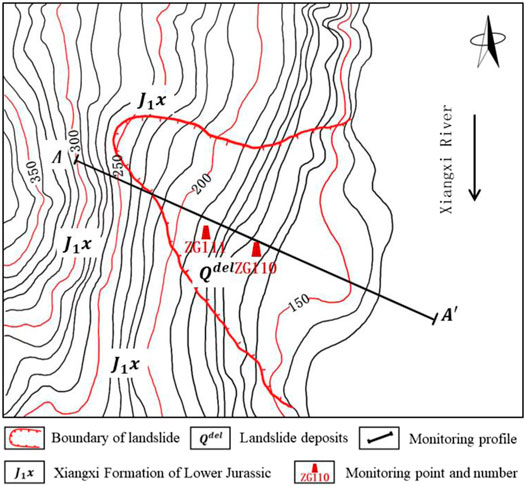
FIGURE 2. Topographical map of the Bazimen landslide, showing the locations of the monitoring points.

Since the Three Gorges Reservoir Area officially began storing water in 2009, the Bazimen landslide has experienced significant deformation with an increasing trend. The growth is characteristic of a typical step-type hydrodynamic landslide (Figure 3). The causes of the landslide’s formation and development are the topography, geology, geologic structure, other engineering geological conditions, rainfall, earthquakes, and reservoir water-level changes. The Bazimen landslide is strongly influenced by the dispatching of the Three Gorges Reservoir, and its cumulative displacement monitoring data have a strong correlation with reservoir water-level changes and the rainfall conditions (Figure 3).

FIGURE 3

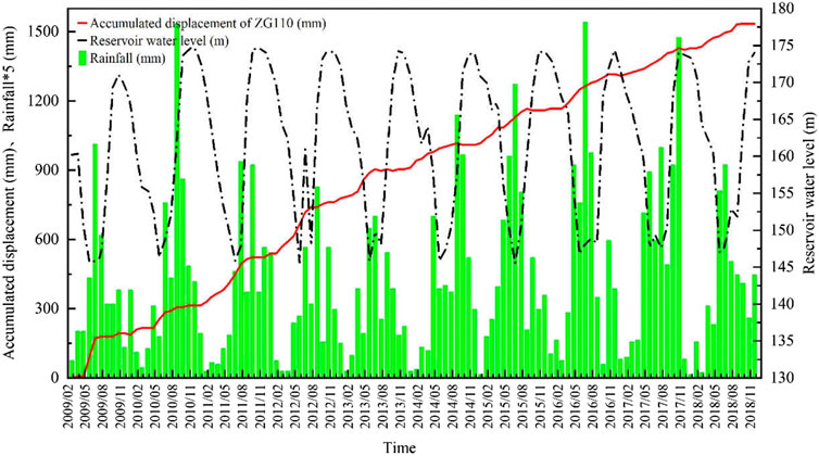
FIGURE 3. Bazimen landslide accumulated displacement, reservoir water level, and rainfall monitoring curve.

On the basis of this understanding, we developed a model to analyze the landslide’s deformation triggers and displacement-related structures using the rainfall and reservoir water-level changes as the basic triggering factors. The Bazimen landslide has multiple monitoring points, among which ZG110 and ZG111 have been monitored for the longest time and are located in the region of the landslide with the largest deformation. The monitoring data for points ZG110 and ZG111 are representative and most accurately represent the development and changes in the landslide displacement. In this study, we selected the monitoring data for point ZG110 for use in the research and analysis. As on December 31, 2018, the cumulative horizontal displacement and cumulative displacement direction of monitoring point ZG110 were 1525.73 mm and 117°, respectively.

Selection of the Influencing Factors

The curves illustrating the relationship between the landslide’s monthly displacement increment, the reservoir’s water-level changes, and the rainfall at monitoring point ZG110 on the Bazimen landslide are shown in Figure 4. As can be seen, at the end of each year when the reservoir’s water level dropped, the landslide deformation rate was extremely high and underwent periodic changes. In addition, the influence of changes in the reservoir’s water level on the landslide deformation was significant.

FIGURE 4

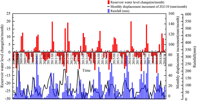
FIGURE 4. Correspondence between the monthly displacement increment of the landslide and the reservoir water-level changes and rainfall at point ZG110.

The effects of the rainfall-and water-level fluctuations on the landslide deformation were as follows. First, the weakening of the landslide’s rocks caused by the rainfall infiltration and the reservoir water infiltration led to the deterioration of the mechanical properties of the landslide and resulted in the deformation of the landslide (Yange et al., 2015). Second, the rainfall infiltration and reservoir water-level fluctuations caused changes in the pressure of the seepage water within the landslide body, which led to the deformation of the landslide (Han et al., 2015). Third, the periodic changes and time effects of the rainfall and reservoir water-level fluctuations also had significant impacts on the landslide deformation (Han et al., 2018). In general, because of the low permeability coefficient of the soil slope, the rainfall infiltration is relatively slow. The influence of long-term rainfall should be fully considered when selecting the influencing factor. We selected the rainfall in the reservoir area in the current month and two months as the influencing factor. The impact of reservoir water is usually a slow process. Therefore, based on the selection of the current monthly change of the current reservoir water level, we also used the two-month cumulative change of the reservoir water level.

Model Evaluation and Optimization

In this study, we selected the Gumbel, Clayton, and Frank Copula functions from the Archimedean Copula family and the M-copula function that linearly combines the three Copula functions as candidates.

First, it was necessary to select the Copula function that best reflects the trends and correlations in the raw data. The first step is the parameter estimation of the model. The Gumbel, Clayton, and Frank Copula models contained one unknown parameter each, and the M-Copula had three coefficients and three function parameters for a total of six parameters to be estimated. Many studies (Motamedi and Liang, 2014; Li et al., 2018; Wang et al., 2020) have used full maximum likelihood estimation (Nelsen, 2000) or the two-step maximum likelihood estimation (Genest et al., 1995) to estimate the model parameters. Both methods required a prior assumption of the type of marginal distribution, which directly affected the structure of the parameter estimation if the marginal distribution was incorrectly selected. In this study, we used the semi-parametric estimation method proposed by Genest (Genest, 1987) and Kim (Kim et al., 2007), that is, the pseudo-MLE method, to estimate the parameters of the Copula model. The parameter estimates are presented in Tables 2, 3. In all of the tables and figures that appear in this paper, the explanation of all the factors and variables are shown as follows (Table 1).

TABLE 1

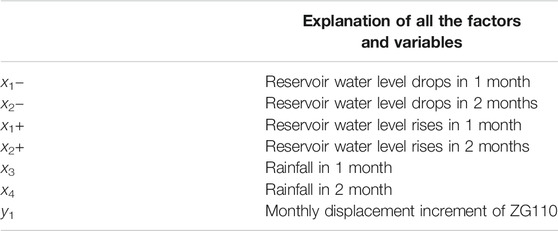
TABLE 1. Explanation of all the factors and variables.

TABLE 2

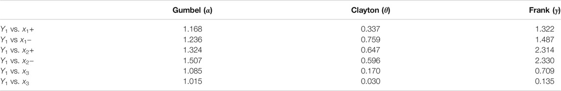
TABLE 2. Parameter estimation for the Gumbel, Clayton, and Frank Copula models.

TABLE 3

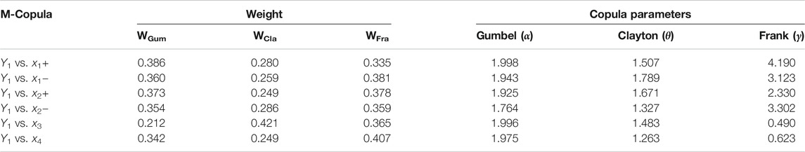
TABLE 3. Parameter estimation for the M-Copula model.

The second step is to select the Copula model with the best fit for the four Copula models according to the AIC and BIC (Wang and Liu, 2006). The calculation results presented in Tables 3, 4 and 5 show that the M-Copula model had the best fit for the data source and thus was chosen for use in the following correlation study.

TABLE 4

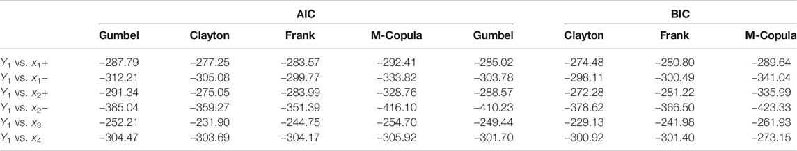
TABLE 4. AIC/BIC values of the Gumbel, Clayton, Frank, and M-Copula models.

TABLE 5

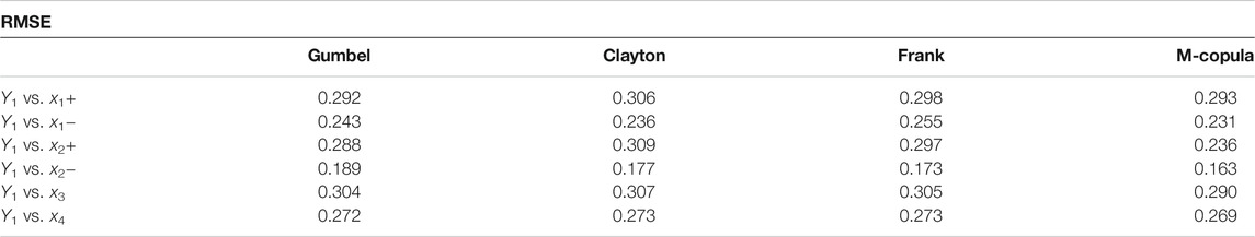
TABLE 5. RMSE values of the Gumbel, Clayton, Frank, and M-Copula models.

We used the K-S test to verify whether the partial derivatives of the M-Copula model obeyed a (0, 1) uniform distribution as a way to check whether the M-Copula model reflected the structure of the correlation between the variables well.

The original hypothesis was that the first-order partial derivatives of the M-Copula model would obey a uniform distribution within (0, 1). We tested the M-Copula function by constructing a K-S test statistic for the M-Copula model. As shown in Table 6, the p-value of the K-S test of the M-Copula model was greater than 0.05 for all six data sets, and the original hypothesis was accepted at the 95% confidence level. Thus, the first-order derivatives of the M-Copula model obeyed a uniform distribution within (0, 1), indicating that the M-Copula model reflected the correlation structure between the variables well.

TABLE 6

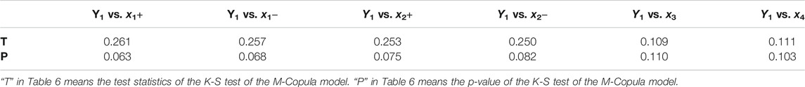
TABLE 6. K-S test results of the M-Copula models.

Correlation Analysis Based on the M-Copula Model

We conducted a correlation analysis of the rainfall and reservoir water-level fluctuations and the landslide deformation using the M-Copula model. Figure 5 shows the spatial density distribution map and density contour metric of the M-Copula model. In all of the figures in this paper, the coordinate axis U represents each influencing factor and V represents the monthly displacement increment of the landslide. Table 7 presents the correlation metric parameters returned by the M-Copula function. Kendall's tau is the Kendall correlation coefficient and was used to show the overall correlation between two sets of random variables. We used the upper-tail and lower-tail coefficients to measure the correlation between the two sets of random variables when the variable became larger or smaller.

FIGURE 5

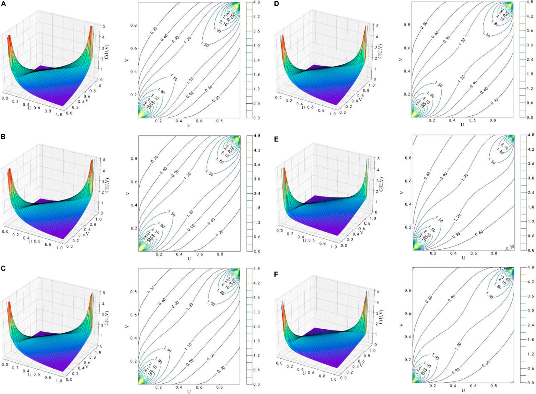
FIGURE 5. (A), Spatial joint density distribution and contour plot between the 2 factors. “Reservoir water level rises in 1 month” and “Monthly displacement increment of ZG110”; (B), Spatial joint density distribution and contour plot between the 2 factors. “Reservoir water level drops in 1 month” and “Monthly displacement increment of ZG110”; (C), Spatial joint density distribution and contour plot between the 2 factors.“Reservoir water level rises in 2 months” and “Monthly displacement increment of ZG110”; (D), Spatial joint density distribution and contour plot between the 2 factors. “Reservoir water level drops in 2 months” and “Monthly displacement increment of ZG110”; (E), Spatial joint density distribution and contour plot between the 2 factors. “Rainfall in 1 month” and “Monthly displacement increment of ZG110”; (F), Spatial joint density distribution and contour plot between the 2 factors. “Rainfall in 2 months” and “Monthly displacement increment of ZG110”.

TABLE 7

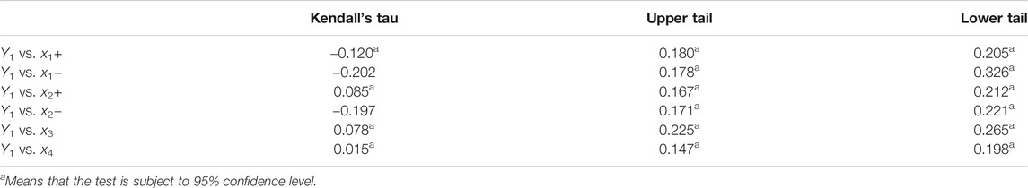
TABLE 7. Relevant parameters of the M-Copula Model.

The correlation parameters calculation results showed that the monthly displacement increment of the landslide was weakly negatively correlated with the one-month change in the reservoir’s water level and the two-month change in the reservoir’s water level, and it was weakly positively correlated with the other influencing factors. Note that the change in the reservoir’s water level in the declining stage was more strongly correlated with the monthly displacement increment of the landslide. The upper-tail correlation coefficient of each group of variables was smaller than the lower-tail correlation coefficient, which is also shown in Figure 6. As the figure shows, the joint probability distribution was thicker in the lower tail and the lower-tail correlation was higher than the upper-tail correlation, indicating that the deformation of the landslide was likely to be smaller when the reservoir water-level fluctuations or rainfall were smaller.

FIGURE 6

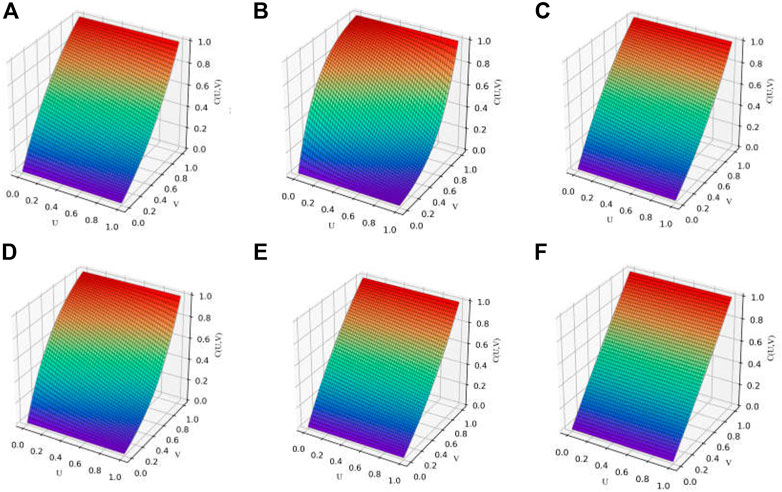
FIGURE 6. Conditional probability density distributions for the M-Copula model. (A)$y_1\hspace{0.17em}\text{vs}.\hspace{0.17em} x_1+$; (B)$y_1\hspace{0.17em}\text{vs}.\hspace{0.17em} x_1-$; (C)$y_1\hspace{0.17em}\text{vs}.\hspace{0.17em}{x}_2+$; (D)$y_1\hspace{0.17em}\text{vs}.\hspace{0.17em}{x}_2-$; (E)$y_1\hspace{0.17em}\text{vs}.\hspace{0.17em}{x}_3$; and (F)$y_1\hspace{0.17em}\text{vs}.\hspace{0.17em}{x}_4$.

Conditional Probability and Return Period of the Landslide Deformation

The conditional probability distribution diagrams and the return period diagrams of the random variables are shown in Figures 6, 7, respectively.

FIGURE 7

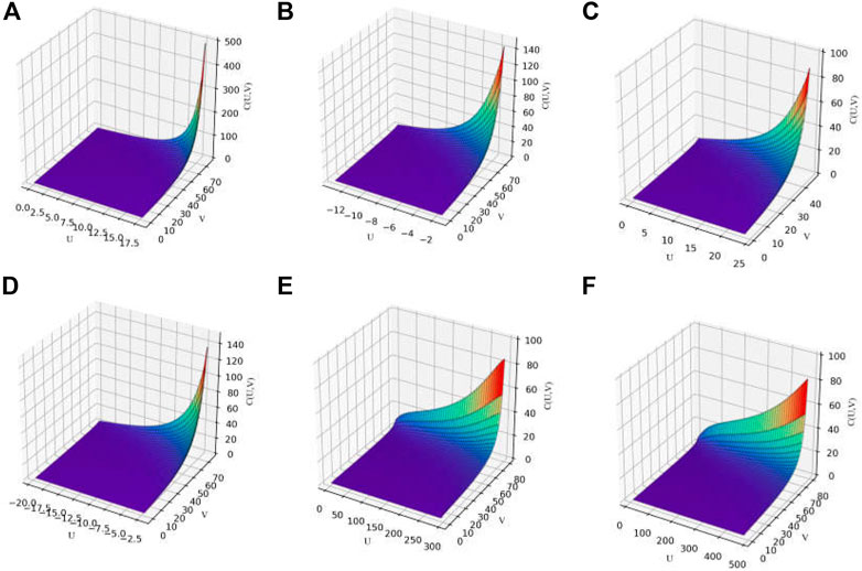
FIGURE 7. Conditional return period diagram for the M-Copula model. (A)$y_1\hspace{0.17em}\text{vs}.\hspace{0.17em} x_1+$; (B)$y_1\hspace{0.17em}\text{vs}.\hspace{0.17em} x_1-$; (C)$y_1\hspace{0.17em}\text{vs}.\hspace{0.17em}{x}_2+$; (D)$y_1\hspace{0.17em}\text{vs}.\hspace{0.17em}{x}_2-$; (E)$y_1\hspace{0.17em}\text{vs}.\hspace{0.17em}{x}_3$; and (F)$y_1\hspace{0.17em}\text{vs}.\hspace{0.17em}{x}_4$.

When the amount by which the reservoir’s water level changes was given, the conditional probability of the monthly displacement increment of the landslide gradually increased as the monthly displacement increment increased. When the amount of rainfall was given, the conditional probability of the monthly displacement increment gradually increased as the monthly displacement increment increased. In terms of the monthly displacement increment, the greater the change in the reservoir’s water or the amount of rainfall, the smaller the probability value.

The return period of the monthly displacement increment of the landslide generally was characterized by a small return period when the change in the reservoir’s water level was large and the monthly displacement increment was small. The return period was small when the amount of rainfall was large and the monthly displacement increment was small, and vice versa. When the reservoir water-level change or the rainfall was given, the return period became progressively larger as the monthly displacement increment increased. When the monthly displacement increment was given, it decreased as the reservoir-level change or rainfall level increased.

We arranged the Bazimen landslide displacement monitoring data in order of magnitude to create a new displacement sequence. The upper quartile of the displacement sequence of the monthly displacement increment of monitoring point ZG110 was 22.42 mm. If the monthly displacement increment was greater than 22.42 mm, we determined that the landslide had a large deformation in this month, and if it was less than 22.42 mm, we considered it to have a small deformation.

On the basis of this division, we reviewed the probability distribution and the return period of the monthly displacement increment for the selected −10 and 20 m monthly reservoir water-level changes, the −20 and 20 m two-month reservoir water-level changes, the 100 and 300 mm monthly rainfall levels, and the 200 and 500 mm two-month cumulative rainfall levels.

As shown in Figure 8A, the probability of a large landslide deformation in a month when the reservoir level dropped by 10 m was the highest (0.965) under various conditions. The probabilities for other changes in the reservoir’s water level are shown in Table 8. Large landslide deformation was most likely to occur when the reservoir’s water level fluctuated significantly, and the probability of a large landslide deformation occurring in a month when the reservoir’s water level dropped was 0.965.

FIGURE 8

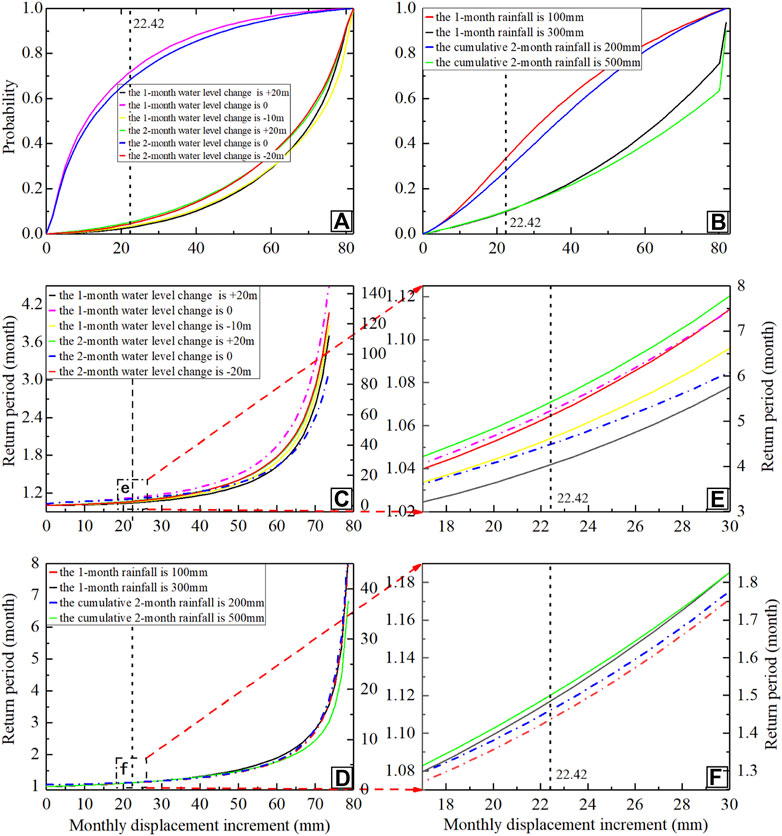
FIGURE 8. Probability distribution and return period plots of the monthly displacement increments for the M-Copula model. (A) conditional probabilities under different reservoir level changes; (B) conditional probability distributions under different rainfall conditions; (C) return periods under different reservoir level changes; (D) locally amplified (C); (E) return periods under different rainfall conditions; and (F) locally amplified (D).

TABLE 8

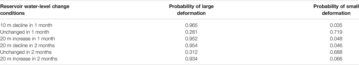
TABLE 8. Probability of landslide deformation under different reservoir level change conditions.

We obtained the following analysis results: When the reservoir’s water level fluctuated significantly, the landslide was likely to experience deformation. In this case, the probability of a large landslide deformation occurring in a month in which the reservoir’s water level dropped was higher than the probability of it occurring in a month in which the reservoir’s water level rose. When the reservoir’s water level remained unchanged, the probability of large landslide deformation occurring was significantly smaller than the probability of reservoir water storage or flooding. A reasonable explanation for this phenomenon was that most of the Bazimen landslides were below 145 m, and a rapid decrease in the reservoir’s water level and the poor permeability of the landslide’s geotechnical body caused the groundwater level within the slope to lag behind the reservoir’s water level. This resulted in a positive difference between the groundwater level and the reservoir’s water level. The outward infiltration of the groundwater from the landslide body caused the osmotic pressure to be directed toward the outside of the slope body. As a result, a significant deformation of the slope body was likely to occur during a sudden drop in the reservoir’s water level.

As shown in Figure 8B, under different rainfall conditions in the reservoir area, the probability of a large landslide deformation occurring was the highest (0.900) when the cumulative rainfall for two months was 500 mm. The probabilities for the other rainfall conditions are shown in Table 9. This analysis led us to the conclusion that the greater the cumulative rainfall for one month or two months in the reservoir area, the more likely it was that the landslide would experience a significant deformation. This phenomenon may have been due to the fact that rainfall that infiltrated the slope increased the weight of the landslide and created pore penetration pressure. Thus, the slip zone soil also was softened by the water, which in turn would reduce its shear strength and cause a significant deformation.

TABLE 9

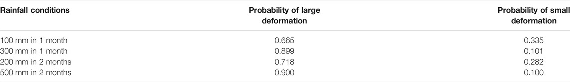
TABLE 9. Probability of landslide deformation under different rainfall conditions.

By comparing the degrees of the influences of the reservoir water-level fluctuations and the rainfall on the landslide displacement in the reservoir, it was evident that changes in the reservoir’s water level, especially when the reservoir’s water level dropped, were more likely to cause large amounts of landslide deformation compared with rainfall for both the one- and two-month conditions.

We analyzed the pattern of the monthly displacement increment return period of the Bazimen landslide under specific conditions. As is shown in Figures 8C,E, the return period of the large landslide deformation (≥22.42 mm) when the reservoir’s water level fluctuated greatly (up or down) was much smaller than the return period when the reservoir’s water level remained unchanged or fluctuated less. Note that the return period for large landslide deformations was smaller when the reservoir’s water level decreased than when the reservoir’s water level increased. This result indicated that the probability of large landslide deformations was greatly increased in the case of sudden decreases in the reservoir’s water level.

As the monthly displacement increment of the landslide increased from 22.42 mm to a maximum of 72.44 mm, the return period of the monthly displacement increment of the landslide increased by less than three months in the case of large fluctuations in the reservoir’s water level. When the reservoir’s water level remained basically unchanged, the return period increased by nearly 10 years. This result indicated that the landslide was more likely to undergo deformation destabilization and cause serious geological hazards when large fluctuations in the reservoir’s water level occurred.

As is shown in Figures 8D,F, the return period of large landslide deformation (≥22.42 mm) was smaller when there was heavy rainfall in the reservoir area than when there was less rainfall. In particular, the return period of extremely large landslide deformation events (close to 75 mm) was much smaller for heavy rainfall than for smaller rainfall, with almost an order of magnitude difference. This indicated that the probability of large landslide deformation increased considerably under the heavy-rainfall scenario. As the monthly displacement increment of the landslide increased from 22.42 mm to a maximum of 72.44 mm, the return period of the monthly displacement increment of the landslide increased by only about seven months in the case of heavy rainfall. In the case of light rainfall, however, it increased by nearly four years. This result indicated that in the case of heavy rainfall, the landslide was also more prone to deformation destabilization and caused serious geological disasters.

Table 10 shows the VaRs, TVaRs and their corresponding displacement increments of all the influencing factors based on the calculations using Eqs 8Eqs 9. On the whole, the displacement increment corresponding to the VaRs and TVaRs of rainfall is smaller than the displacement increment corresponding to the VaRs and TVaRs of reservoir level change, indicating that the response of landslide deformation to reservoir level change is higher than the response to rainfall. Moreover, the increment of displacement corresponding to VaRs and TVaRs when the reservoir level is falling is greater than that when it is rising. It can be assumed that landslide deformation responds more to a fall than to a rise in reservoir water level. When the four influencing factors reached or exceeded their respective VaR, the possibility of a large amount of landslide deformation occurring was greater. At that moment, it would be necessary to pay more attention to the landslide deformation and corresponding landslide geohazard emergency measures should be taken.

TABLE 10

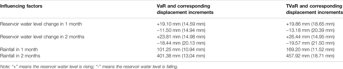
TABLE 10. VaRs and TVaRs of influencing factors.

Case Validation: Baishuihe Landslide

The Baishuihe landslide is another typical landslide in the Three Gorges Reservoir area, located on the south bank of the Yangtze River in Zigui County, and its deformation development is mainly influenced by a combination of factors such as reservoir water level changes and rainfall. Monitoring data from the Baishuihe landslide from 2009 to 2018 were selected to verify the effectiveness of the proposed pseudo MLE-M-Copula approach. First, the monitoring data of monthly displacement increment, reservoir level changes and rainfall at monitoring point ZG118 were tested for normality using A-D test, J-B test and KS test. The p values of all variables were less than 0.05, indicating that none of the variables obeyed normal distribution and there is tail correlation between two variables. The M-Copula model proposed in this paper was used to fit the data, and the best fit was obtained on all candidate models based on three evaluation indicators: AIC, BIC and RMSE. The Kendall’s τ and the tail correlation coefficients between each influencing factor and the monthly displacement increment were then calculated (Table 11), and it can be concluded that the monthly displacement increment is weakly negatively correlated with the reservoir level change (rise or fall) and weakly positively correlated with rainfall, which is basically the same as that of the Bazimen landslide. And the decrease in reservoir level has a stronger correlation with the incremental displacement. In addition, the upper tail correlation coefficient of variables is greater than the lower tail correlation coefficient. Unlike the Bazhimen landslide, the upper tail correlation of the displacement increment of the Baishuihe landslide with the influencing factors is higher than the lower tail correlation, indicating that when the reservoir water level changes or the rainfall is greater, the landslide is more likely to have large deformation. Finally, the VaRs and TVaRs of displacement increments and each influencing factor were calculated (Table 12), the results were roughly the same as the Bazhimen landslide, but the displacement increments were more responsive to rainfall. In summary, there are good reasons to believe that the M-Copula model based on pseudo-MLE proposed in this paper can effectively and accurately evaluate the correlation between the influencing factors and deformation of hydrodynamic landslides in the TGRA.

TABLE 11

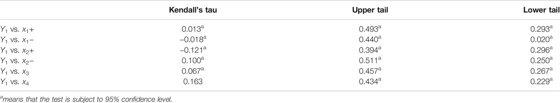
TABLE 11. Relevant parameters of the M-Copula Model.

TABLE 12

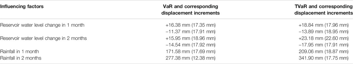
TABLE 12. VaRs and TVaRs of influencing factors.

Discussion

In this paper, we proposed a new M-Copula method based on pseudo-MLE to systematically investigate the correlation between landslide influencing factors and deformation of the Bazimen landslide in the TGRA. The method offered several advantages. First, the Copula method is based on nonlinear theory and can be used to completely characterize the correlation structure between multidimensional random variables. Second, the hybrid M-Copula method combined the advantages of three different Archimedean Copula functions to provide a more comprehensive and accurate description of the complex correlations. In addition, the pseudo-MLE method used to estimate the parameters of the model was able to avoid the adverse effects on the analysis results caused by the incorrect selection of the marginal distribution. Third, the introduction of conditional probability distributions and return periods allowed for a more accurate description of the effect of one variable on landslide deformation when one variable was fixed.

This method also had limitations. First, the selection of influencing factors was largely dependent on empirical and qualitative analysis, and lacked concrete and computational support. Second, the study examined only the correlation between the monthly displacement increments of single monitoring point data and the influencing factor, and failed to consider the spatial characteristics of the landslide. Third, data from several monitoring points at different locations should be added to analyze the correlation structure between the three-dimensional spatial characteristics of the landslide and the landslide deformation, given that this study did not consider the changes in landslide displacement under the joint action of multiple influencing factors.

Conclusion

In this research, a Mixed-Copula method based on pseudo-maximum likelihood estimation is proposed to monitor and study the correlation between landslide displacements and their various influencing factors (including rainfall, reservoir water level changes). Monitoring data collected from 2009 to 2018 from the Bazimen landslide in the Three Gorges Reservoir area were used to develop probabilistic statistical models between landslide deformation and its influencing factors using Archimedeans Copula and Mixed Copula models, respectively, and to conduct numerical analysis.

The M-Copula model was firstly developed using a semi-parametric estimation method (pseudo MLE) based on the monitoring data and compared with parametric and non-parametric estimation methods. In order to select the best-fit model on the monitoring data and to confirm its validity and accuracy, the M-Copula model was then compared with the Frank, Gumbel and Clayton copula models on the monitoring data. Three evaluation metrics, AIC, BIC and RMSE, were chosen to assess the goodness-of-fit, with the M-Copula model achieving the best results. These models were tested for statistical hypotheses using the A-D test, J-B test and KS-test. Through correlation analysis, including overall correlation analysis and tail correlation analysis, it was found that the tail correlation was greater than the overall correlation and that the lower tail correlation was greater than the upper tail correlation. This result indicated that the possibility of a decrease in the displacement increment was significantly enhanced when there was a large decrease in the reservoir’s water level or the amount of rainfall in the reservoir area. VaRs and TVaRs were used to calculate the threshold values for each influencing factor and its corresponding landslide displacement.

The results of the computational study validate the ability of the pseudo MLE-M-Copula model to analyze landslide deformation correlations and it can be well applied to other landslides in the same reservoir area. According to the results of the correlation calculations (tail correlation, conditional probability and return period, VaR and TVaR), there is a significant correlation between the landslide deformation, i.e., the landslide displacement increment, and the sudden drop of the reservoir water level, heavy rainfall. Therefore, the prevention of landslide hazards can be predicted by enhancing the monitoring of reservoir level changes and rainfall.

Data Availability Statement

The raw data supporting the conclusions of this article will be made available by the authors, without undue reservation.

Author Contributions

1) The contribution of RW is the idea, introduction, theory and methodology, overview of the Bazimen Landslide, monitoring data analysis, conclusions. 2) The contribution of KZ is the relevance analysis. 3) The contribution of JQ is the programming of relevance analysis. 4) The contribution of WX is the displacement mechanism manof hydrodynamic landslide. 5) The contribution of Huanling Wang is the theory and methodology of Copula 5) The contribution of HH is the monitoring data analysis of Bazimen Landslide.

Funding

This work is supported by the National Natural Science Foundation of China (No.51939004), the Fundamental Research Funds for the Central Universities (No. B200204008), the Open Foundation of National Field Observation and Research Station of Landslides in the TGRA of Yangtze River, China Three Gorges University (2018KTL03).

Conflict of Interest

The authors declare that the research was conducted in the absence of any commercial or financial relationships that could be construed as a potential conflict of interest.

Acknowledgments

We thank the National Field Observation and Research Station of Landslides in the TGRA of Yangtze River for their help in providing monitoring data for this study.

References

Ahmed, B. (2015). Landslide susceptibility mapping using multi-criteria evaluation techniques in Chittagong Metropolitan Area, Bangladesh. Landslides 12, 1077–1095. doi:10.1007/s10346-014-0521-x

CrossRef Full Text | Google Scholar

Bai, S. B., Wang, J., Lue, G., Zhou, P. G., Hou, S. S., and Xu, S. N. (2010). GIS-based logistic regression for landslide susceptibility mapping of the Zhongxian segment in the Three Gorges area, China. Geomorphology 115, 23–31. doi:10.1016/j.geomorph.2009.09.025

CrossRef Full Text | Google Scholar

Bezak, N., Raj, M., and Miko, M. (2016). Copula-based IDF curves and empirical rainfall thresholds for flash floods and rainfall-induced landslides. J. Hydrol. 541, 272–284. doi:10.1016/j.jhydrol.2016.02.058

CrossRef Full Text | Google Scholar

Cai, Z., Xu, W., Meng, Y., Shi, C., and Wang, R. (2016). Prediction of landslide displacement based on GA-LSSVM with multiple factors. Bull. Eng. Geology. Environ. 75, 637–646. doi:10.1007/s10064-015-0804-z

CrossRef Full Text | Google Scholar

Cao, Y., Yin, K., Alexander, D. E., and Zhou, C. (2016). Using an extreme learning machine to predict the displacement of step-like landslides in relation to controlling factors. Landslides 13, 725–736. doi:10.1007/s10346-015-0596-z

CrossRef Full Text | Google Scholar

Chen, Z., Zhang, J., Li, Z., Wu, F., and Ho, K. (2008). Landslides and engineered slopes. From the past to the future (proceedings of the 10th international symposium on landslides and engineered slopes, 30 june-4 july 2008, xi’an, China). 3D landslide run out Model. using Part. Flow Code PFC3D, 873–879. doi:10.1201/9780203885284

CrossRef Full Text | Google Scholar

Christian, G., and Bruno, B. (2008). Validity of the parametric bootsrap for goodness-of-fit testing in semiparametric models. Ann. Inst. H. Poincare Probab. Statist 44, 1096–1127. doi:10.1214/07-AIHP148

CrossRef Full Text | Google Scholar

Dempster, A. P., Laird, N. M., and Rubin, D. B. (1977). Maximum-likelihood estimation from incomplete data via the EM algorithm (with discussion). J. R. Stat. Soc. Ser. B: Methodological 39, 1–38. doi:10.2307/2984875

CrossRef Full Text | Google Scholar

Genest, C. (1987). Frank's family of bivariate distributions. Biometrika 74, 549–555. doi:10.2307/2336693

CrossRef Full Text | Google Scholar

Genest, C., Ghoudi, K., and Rivestal, P. (1995). A semiparametric estimation procedure of dependence parameters in multivariate families of distributions. Biometrika 3. doi:10.2307/2337532

CrossRef Full Text | Google Scholar

Han, Z., Chen, G., Li, Y., and He, Y. (2015). Numerical simulation of debris-flow behavior incorporating a dynamic method for estimating the entrainment. Eng. Geology. 190, 52–64. doi:10.1016/j.enggeo.2015.02.009

CrossRef Full Text | Google Scholar

Han, Z., Wang, W., Li, Y., Huang, J., Su, B., Tang, C., et al. (2018). An integrated method for rapid estimation of the valley incision by debris flows. Eng. Geology. 232, 34–45. doi:10.1016/j.enggeo.2017.11.007

CrossRef Full Text | Google Scholar

Hong, H., Pourghasemi, H. R., and Pourtaghi, Z. S. (2016). Landslide susceptibility assessment in Lianhua County (China): a comparison between a random forest data mining technique and bivariate and multivariate statistical models. Geomorphology 259, 105–118. doi:10.1016/j.geomorph.2016.02.012

CrossRef Full Text | Google Scholar

Hu, L. (2002). Essays in econometrics with applications in macroeconomic and financial modelling. New Haven: Yale University

Iyengar, S. (1997). Multivariate models and dependence concepts. New York: Chapman & Hall

Kafri, U., and Shapira, A. (1990). A correlation between earthquake occurrence, rainfall and water level in Lake Kinnereth, Israel. Phys. Earth Planet. Interiors 62, 283. doi:10.1016/0031-9201(90)90172-T

CrossRef Full Text | Google Scholar

Kawamoto, O. (2005). Finite element method for landslide analysis No. 14 : application of FEM for landslide analysis. J. Jpn. Landslide Soc. 42, 657–660. doi:10.3313/jls.42.85

CrossRef Full Text | Google Scholar

Kim, G., Silvapulle, M. P., and Silvapulle, J. (2007). Comparison of semiparametric and parame- tric methods for estimating copulas. Comput. Stat. Data Anal. 51, 2836–2850. doi:10.1016/j.csda.2006.10.009

CrossRef Full Text | Google Scholar

Kirschbaum, D. B., Adler, R., Hong, Y., Hill, S., and Lerner-Lam, A. (2010). A global landslide catalog for hazard applications: method, results, and limitations. Nat. Hazards 52, 561–575. doi:10.1007/s11069-009-9401-4

CrossRef Full Text | Google Scholar

Li, H., Xu, Q., He, Y., and Deng, J. (2018). Prediction of landslide displacement with an ensemble-based extreme learning machine and copula models. Landslides 15, 2047–2059. doi:10.1007/s10346-018-1020-2

CrossRef Full Text | Google Scholar

Liu, X., and Zhang, Q. (2016). Analysis of the return period and correlation between the reservoir-induced seismic frequency and the water level based on a copula: a case study of the Three Gorges reservoir in China. Phys. Earth Planet. Interiors 260, 32–43. doi:10.1016/j.pepi.2016.09.001

CrossRef Full Text | Google Scholar

Lollino, P., Elia, G., Cotecchia, F., and Mitaritonna, G. (2010). Analysis of landslide reactivation mechanisms in Daunia clay slope by means of limit equilibrium and FEM methods. San Diego, CA: Geotechnical Special Publication, 3155–3164.

Ma, J., Tang, H., Hu, X., Bobet, A., Zhang, M., Zhu, T., et al. (2016). Identification of causal factors for the Majiagou landslide using modern data mining methods. Landslides 14, 1–12. doi:10.1007/s10346-016-0693-7

CrossRef Full Text | Google Scholar

Mackay, C. G. J. (1986). Copules archimédiennes et familles de lois bidimensionnelles dont les marges sont données. Can. J. Stat. 14, 145–159. doi:10.2307/3314660

CrossRef Full Text | Google Scholar

Miao, F., Wu, Y., Xie, Y., and Li, Y. (2017). Prediction of landslide displacement with step-like behavior based on multialgorithm optimization and a support vector regression model. Landslides 15, 475–488. doi:10.1007/s10346-017-0883-y

CrossRef Full Text | Google Scholar

Miyagi, T., Yamashina, S., Esaka, F., and Abe, S. (2011). Massive landslide triggered by 2008 Iwate-Miyagi inland earthquake in the Aratozawa Dam area, Tohoku, Japan. Landslides 8 (1), 99–108. doi:10.1007/s10346-010-0226-8

CrossRef Full Text | Google Scholar

Motamedi, M., and Liang, R. Y. (2014). Probabilistic landslide hazard assessment using Copula modeling technique. Landslides 11, 565–573. doi:10.1007/s10346-013-0399-z

CrossRef Full Text | Google Scholar

Nelsen, R. (2000). An introduction to copulas. Technometrics 42, 272–286. doi:10.2307/1271100

CrossRef Full Text | Google Scholar

Nelsen, R. B. (1986). Properties of a one-parameter family of bivariate distributions with specified marginals. Commun. Stat. Theor. Methods 15, 3277–3285.

CrossRef Full Text | Google Scholar

Ohtake, M. (1986). Seismicity change associated with the impounding of major artificial reservoirs in Japan. Phys. Earth Planet. Interiors 44, 87–89.

CrossRef Full Text | Google Scholar

Pavan, J., Ramana, D., Chadha, R. K., Singh, C., and Shekar, M. (2012). The relation between seismicity and water level changes in the Koyna-Warna region, India. Nat. Hazards Earth Syst. Sci. 12 813–817. doi:10.5194/nhess-12-813-2012

CrossRef Full Text | Google Scholar

Reboredo, J. C. (2011). How do crude oil prices co-move? A copula approach. Energ. Econ. 33, 948–955. doi:10.1016/j.eneco.2011.04.006

CrossRef Full Text | Google Scholar

Rockafellar, R. T., and Uryasev, S. (2002). Conditional value-at-risk for general loss distributions. J. Banking Finance 26, 1444–1471. doi:10.2139/ssrn.267256

CrossRef Full Text | Google Scholar

Shiuan, W. (2012). Entropy-based particle swarm optimization with clustering analysis on landslide susceptibility mapping. Environ. Earth Sci. 68, 1349–1366. doi:10.1007/s12665-012-1832-7

CrossRef Full Text | Google Scholar

Sklar, A. (1959). Fonctions de Repartition an Dimensions et Leurs Marges. Paris: de l’Institut Statistique de l’Université de Paris, 229–231.

Tang, D., Li, D., and Cao, Z. (2017). Slope stability analysis in the Three Gorges Reservoir Area considering effect of antecedent rainfall. Georisk: Assess. Management Risk Engineered Syst. Geohazards 11, 161–172. doi:10.1080/17499518.2016.1193205

CrossRef Full Text | Google Scholar

Telesca, L., ElBary, R. E. F., Mohamed, A. E. A., and ElGabry, M. (2012). Analysis of the cross-correlation between seismicity and water level in the Aswan area (Egypt) from 1982 to 2010. Nat. Hazards Earth Syst. Sci. 12, 2203–2207. doi:10.5194/nhess-12-2203-2012

CrossRef Full Text | Google Scholar

Varnes, D. J. (1996). Landslide types and processes. Landslides-Investigation and Mitigation 247, 36–75.

Google Scholar

Wang, Y., and Liu, Q. (2006). Comparison of Akaike information criterion(AIC) and Bayesian information criterion(BIC) in selection of stock-recruitment relationships. Fish. Res. 77, 220–225. doi:10.1016/j.fishres.2005.08.011

CrossRef Full Text | Google Scholar

Wang, Y., Wen, T., Tang, H., Ma, J., Zhang, J., and Niu, X. (2020). Displacement prediction of a complex landslide in the three gorges reservoir area (China) using a hybrid computational intelligence approach. Complexity 2020, 1–15. doi:10.1155/2020/2624547

CrossRef Full Text | Google Scholar

Wang, Y., Yin, K., and An, G. (2004). Grey correlation analysis of sensitive factors of landslide. Rock Soil Mech. 25, 91–93. doi:10.3969/j.issn.1000-7598.2004.01.019

CrossRef Full Text | Google Scholar

Wu, J., Liu, C., and Qiu, X. X. (2009). Application of extreme value copula functions for measuring bivariate tail dependence. China: School of Mathematics and StatisticsHuazhong University of Science and Technology, 430074

Yan, J. (2006). “Multivariate modeling with copulas and engineering applications,” in Springer handbook of engineering statistics, 973–990. doi:10.1007/978-1-84628-288-1_51

CrossRef Full Text | Google Scholar

Yange, L., Han, Z., Chen, G., and HE, Y. (2015). Assessing entrainment of bed material in a debris-flow event: a theoretical approach incorporating Monte Carlo method. Earth Surf. Process. Landforms: J. Br. Geomorphological Res. Group 40, 1877–1890. doi:10.1002/esp.3766

CrossRef Full Text | Google Scholar

Yin, Y., Wang, F., and Ping, S. (2009). Landslide hazards triggered by the 2008 Wenchuan earthquake, Sichuan, China. Landslides 6, 139–152. doi:10.1007/s10346-009-0148-5

CrossRef Full Text | Google Scholar

Zhang, L., and Singh, V. P. (2007a). Bivariate rainfall frequency distributions using Archimedean copulas. J. Hydrol. 332, 109. doi:10.1016/j.jhydrol.2006.06.033

CrossRef Full Text | Google Scholar

Zhang, L., and Singh, V. P. (2007b). Gumbel–hougaard copula for trivariate rainfall frequency analysis. J. Hydrologic Eng. 12, 409–419. doi:10.1061/(ASCE)1084-0699(2007)12:4(409)

CrossRef Full Text | Google Scholar

Zhou, C., Yin, K., Cao, Y., and Ahmed, B. (2016). Application of time series analysis and PSO–SVM model in predicting the Bazimen landslide in the Three Gorges Reservoir, China. Eng. Geology. 204, 108–120. doi:10.1016/j.enggeo.2016.02.009

CrossRef Full Text | Google Scholar