Continuous-Flow Analysis of δ17O, δ18O, and δD of H2O on an Ice Core from the South Pole

1 Introduction

Measurements of the isotopes of hydrogen and oxygen of water from ice cores provide important records of past climate (Dansgaard, 1964). Both δD and δ¹⁸O have long been used as proxies for temperature (Jouzel et al., 1997). The relationship between δD and δ¹⁸O in precipitation is nearly linear, but deviations from the average global relationship, defined as the “deuterium excess”, provide valuable additional information (Merlivat and Jouzel, 1979). The deuterium excess is sensitive to kinetic fracationation processes that occur during evaporation when the air is undersaturated, and the combined use of δD and δ¹⁸O can therefore be used to determine past temperature and humidity variations at the ocean surface (Johnsen et al., 1989; Petit et al., 1991; Vimeux et al., 2001; Jouzel et al., 2007; Markle et al., 2017).

Analytical methods developed relatively recently (Barkan and Luz, 2005; Schoenemann et al., 2013; Steig et al., 2014; Schauer et al., 2016) have made possible the addition of δ¹⁷O and “¹⁷O excess” (Δ¹⁷O) measurements in ice cores. These variables are of interest for several reasons. First, because Δ¹⁷O is less sensitive to temperature than deuterium excess, it can help to disentangle the competing effects of temperature and humidity in contributing to the signal at the point of evaporation (Barkan and Luz, 2007; Landais et al., 2008; Winkler et al., 2012). Second, the combined use of d and Δ¹⁷O helps to constrain the degree of supersaturation of water over ice in cold clouds, a long-standing problem for the modeling of water isotopes in polar precipitation (Jouzel and Merlivat, 1984; Risi et al., 2013; Schoenemann et al., 2014; Dütsch et al., 2019), and also of interest more generally for cloud microphysics studies because of the strong fractionation that occurs during ice-cloud formation, particulary important to climate in the tropics (Webster and Heymsfield, 2003). Multiple-isotope studies have also proven useful, for example, in the study of water evapotranspiration and non-rainfall precipitation (i.e., fog, dew) (Kaseke et al., 2017). Finally, analyses of the spectral properties of the water isotope signals in ice cores can be used to constrain past conditions in the firn (the layer of dry porous snow at the surface of polar ice sheets), based on the diffusive process that the water isotopic signal undergoes in the firn layer (Gkinis et al., 2014; Holme et al., 2018; Kahle et al., 2018). In principle, δ¹⁷O can provide a greater signal-to-noise ratio than δ¹⁸O for such applications (Simonsen et al., 2011).

Measurement of water isotope ratios has traditionally been done by isotope ratio mass spectrometry (IRMS) (Epstein and Mayeda, 1953; Coplen et al., 1991; Barkan and Luz, 2005). For ice core research, IRMS has been replaced in many laboratories by laser absorption spectroscopy methods (Kerstel et al., 1999; Gkinis et al., 2011). A key advantage of laser spectroscopy is that it permits the continuous measurement of ice cores, providing increased spatial (i.e., depth) resolution, reduced sample-processing costs, and better compatibility with other measurement systems such as those used for obtaining ion and gas-concentration data (e.g., Schüpbach et al., 2009; Bigler et al., 2011). The original methods developed by Gkinis et al. (2010; 2011) were adapted by, e.g., Maselli et al. (2013) and Emanuelsson et al. (2015) and extended by Jones et al. (2017b) to obtain the first complete ice core record measured continuously at very high resolution; the West Antarctica Ice Sheet (WAIS) Divide record resolves δD and δ¹⁸O at better than 0.5 cm resolution. This provides subannual resolution for more than 30,000 years, and subdecadal resolution for more than 60,000 years (Jones et al., 2017a; Jones et al., 2018).

In this paper, we describe measurements of the complete suite of water isotope ratios on an ice core at the South Pole. We use the laser spectroscopy instrument developed by Steig et al. (2014), and sold commericially as the Picarro L2140-i, coupled to the continuous-flow system developed by Jones et al. (2017b). Schauer et al. (2016) have previously shown the L2140-i to be capable of routine measurements on discrete water samples at sufficient precision to determine Δ¹⁷O, which requires at least an order of magnitude better precision that is normally required for δ¹⁸O. Continuous-flow analysis of ice-core δ¹⁷O and Δ¹⁷O has not been previously described. We briefly highlight notable aspects of the South Pole isotope records, with emphasis on deuterium excess and Δ¹⁷O, but refer to future work for more complete discussion of the paleoclimate interpretation of our results. Our primary goal in this paper is to detail measurement protocols, describe the calibration procedures, and consider the strengths as well as the limitations of the continuous-flow approach for the measurement of the complete suite of water-isotope ratios.

2 Materials and Methods

2.1 Notation

We use the following notation for isotopic abundances, reported as deviations from the water isotope standard, Vienna Mean Standard Ocean Water (VSMOW):

${\delta }^{18}\text{O}=\frac{{}^i{R}_{sample}}{{}^i{R}_{VSMOW}},\delta D=\frac{{}^2{R}_{sample}}{{}^2{R}_{VSMOW}}(1)$

where i = {17,18}, ⁱR = n(ⁱO)/n¹⁶(O), ²R = n(²H)/n(¹H), and n denotes isotope abundance.

Deuterium excess, in its conventional linear (Merlivat and Jouzel, 1979) and empirical logarithmic (Uemura et al., 2012) forms, are given respectively by:

$d=\delta \text{D}-8\left({\delta }^{18}\text{O}\right)(2)$

and

$d_{ln}=ln\left(\delta \text{D}+1\right)-8.47\left(ln\left({\delta }^{18}\text{O}+1\right)\right)-28.5{\left(ln\left({\delta }^{18}\text{O}+1\right)\right)}^2(3)$

The ¹⁷O excess (Δ¹⁷O) is defined as (Barkan and Luz, 2005):

${\text{Δ}}^{17}\text{O}=ln\left({\delta }^{17}\text{O}+1\right)-0.528\left(ln\left({\delta }^{18}\text{O}+1\right)\right)(4)$

All reported isotope values are normalized to the composition of SLAP (Standard Light Antarctic Precipitation), and are therefore on the VSMOW-SLAP scale. The isotopic values for SLAP, relative to VSMOW, are given by δ¹⁸O = −55.5‰, δD = −428‰ and δ¹⁷O = −29.6986‰, following convention (Gonfiantini, 1978; Coplen, 1988; Schoenemann et al., 2013). Note that the δ¹⁷O of SLAP is defined by Δ¹⁷O ≡ 0 (Schoenemann et al., 2013). For all water δ and Δ values, VSMOW ≡ 0. Although Schoenemann et al. (2013) recommends using explicit terminology (e.g., δ¹⁷O_VSMOW−SLAP) to make it clear that the VSMOW-SLAP normalization is used, for simplicity we use more concise terminology (e.g. δ¹⁷O for uncalibrated data, δ¹⁷O_VSMOW for calibrated data).

2.2 Ice Core Samples

We obtained an ice core at 89.99^°S, 98.16^°W, approximately 2 km from the geographic South Pole, during the 2014–2015 and 2015–2016 austral summers (Johnson et al., 2020; Souney et al., 2020). The core, “SPC14”, was drilled to a depth of 1751 m, equivalent to an age of approximately 54 ka. The modern accumulation rate at South Pole is 8 cm w. e. yr⁻¹ (Casey et al., 2014), and the mean annual temperature is −51^°C (Severinghaus et al., 2001). A depth-age relationship for the core, tied directly to the timescale for the WAIS Divide ice core (WAIS Divide Project Members, 2013; WAIS Divide Project Members, 2015), was developed by Winski et al. (2019) and is termed the “SP19” chronology. A timescale for the gas within the core is also available (Epifanio et al., 2020).

We sampled SPC14 in 1 m long sections, with the resulting ice sticks measuring 1.3 × 1.3 cm in square cross section. The small volume of ice used allowed us to sample some sections of the core in duplicate, so that additional samples could be used for replicate measurements. For continuous-flow measurements, each 1 m ice stick was stored in a 1.9 × 1.9 cm square acrylic tube that was loaded vertically onto a melting device, described in the next section. For a limited number of replicate measurements, ice was melted in 1/2 m sections in clean HDPE bottles and decanted into 1 ml vials for later analysis.

2.3 Measurement System and Analysis Protocol

We analyzed the entire South Pole ice core (depth 0–1751 m) for δ¹⁸O and δD. For δ¹⁷O, we analyzed the core from 556 to 1751 m only; the necessary instrument was not available at the time of the first analysis campaign.

For continuous-flow analysis (CFA), we use the system developed and described in detail by Jones et al. (2017b). Briefly, ice core samples in acrylic tubes are placed vertically on an aluminum block melter that has two concentric catchments that channel meltwater into a small drain. The melter is maintained at 14.6±0.1 C. Liquid water is drawn away from the melter using a peristaltic pump and pushed through an 8 μm filter. The filtered water then enters a 2 ml open-top glass vial where bubbles can escape. The water enters a six-port selection valve, and is mixed with high-pressure (80 psi) dry air in a glass concentric nebulizer, where it is converted into a fine spray. The spray enters a 20.0 × 1.8 cm Pyrex vaporizing tube heated to 200 C, and additional dry air (<30 ppm H₂O) is added at a rate of 3.5 L/min to dilute the water vapor and achieve a final water vapor content of ∼25,000 ppm H₂O. For our measurements the target value of 25,000 was maintained within ± 3,500 ppm, with rare values below 10,000 ppm flagged and excluded. The water vapor enters two intake lines (3.175 mm OD × 2 mm ID × 10 cm stainless-steel tubing), each inserted approximately 5 cm into the Pyrex vaporizing tube, which acts as an open split such that excess water vapor is vented to the laboratory. Each intake line is plumbed into a different laser spectroscopy instrument, a Picarro L2130-i and a Picarro L2140-i.

Both the L2130-i and L2140-i instruments are based on the earlier design described by Crosson (2008). These instruments use cavity ring-down spectroscopy (CRDS), in which the abundance of a given target molecule in an optical cavity is determined by pulsing a laser source at 10²–10³ Hz though the cavity. At the end of each pulse, the intensity of infrared light decays exponentially; the e-folding length of the decay is the “ring-down” time, which is proportional to the abundance of the target molecule. In the L2130-i, the ¹H₂¹⁶O, ²H¹H¹⁶O, and ¹H₂¹⁸O isotopogues are detected from the ring-down time for a single laser operating at wavenumbers in the range of 7,200 cm⁻¹. In the L2140-i, a second laser, centered on 7,193 cm⁻¹ where there are stronger absorption lines for ¹H₂¹⁷O, is also used. Rapid switching between the two lasers allows the measurement of all four isotopologues. The L2140-i uses peak-area integration rather than peak height (as used by L2130-i) to determine isotopologue abundance ratios, and laser resonance in the optical cavity is achieved by a different method, as described in detail in Steig et al. (2014). We use both instruments in our measurements because the use of the L2130-i in continuous-flow analysis of ice cores is well established (Jones et al., 2017b), and serves as a reference point for the quality of the δD and δ¹⁸O measurements in either instrument.

Measurements of the South Pole ice core using the CFA system follows essentially the same protocol described in Jones et al. (2017b), with the addition of the L2140-i. Water flow from the ice core can be switched off at a six-port Valco value, allowing flow from 30 ml glass vials that contain laboratory reference waters. At the end of each day, the laboratory reference waters whose values are known relative to the VSMOW standards are run for 40 min each (We also ran reference waters at the beginning of each day in the first year of analysis, but found that this provided no additional benefit). Values of the laboratory reference waters are given in Table 1. The reference waters “KAW”, “KPW” and “WW” were analyzed twice each day; “VW1f” was analyzed once. To characterize isotopic mixing, three small (20 cm × 1.3 × 1.3 cm) sections of laboratory-prepared ice are made from batches of isotopically distinct waters with δ¹⁷O values of approximately −14‰ for the first and third sections and −5‰ for the second section. Additionally, each set of several cores is separated by a 20 cm section of ice with a δ¹⁷O value of about −14‰, which we refer to as “push ice”. This provides an easily identified signal so that ice cores can be distinguished in the data stream. In addition to the daily standards and ice core samples, we also ran longer measurements of reference waters at the end of each week, both to ensure that water continued to flow through the system when it was not being used for ice-core analysis, and to obtain additional data for evaluation of the system for inter-laboratory comparison.

TABLE 1

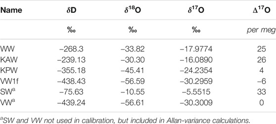
TABLE 1. Isotopic values of reference waters.

A number of routine performance metrics were used to monitor the quality of the CFA measurements and to produce “raw” data sets that are calibrated against the reference waters. Each meter of ice takes approximately 40 min to melt, and data are generated nominally at 1 Hz, resulting in approximately 2,400 data points per meter. Each data point is assigned to a specific depth using a depth-assignment algorithm; depths are provided by readout from a digital laser-distance meter. Raw data are flagged for exclusion where they do not meet metrics such as reproducibility and water concentration targets in the Picarro instrument, and other criteria such as the timing of valve switches (which can introduce spurious noise); details are given in Jones et al. (2017b) and Steig et al. (2020). A final data set is produced by averaging all non-flagged data points over 0.5 cm intervals, after calibration (see next section). Jones et al. (2017b) developed a methodology for correcting measurements for memory; this affects samples that are measured immediately after the “push ice”. We do not use memory correction but instead remove data obtained within 200 s of a large isotopic transition (e.g., after the switch from push ice to sample); the cut-off time is based on measurements of laboratory-created ice of known composition. Memory-correction data are available in the data archive (Steig et al., 2020).

For measurements of discretely sampled ice, we used a Picarro L2140-i with an autosampler, following the protocols given in Schauer et al. (2016). Briefly, 1.8 μl of water are injected using a 10 μl syringe into a vaporization module with a liquid autosampler. The vaporizer-provided mixture of water vapor and dry air is pulled into the laser cavity with a diaphragm pump. A “run” is defined as a set of vials automatically sampled sequentially from start to finish. Each run containing unknown samples is organized by having a set of five reference waters, n samples (typically n∼30 vials), and then another set of five reference waters. Reference waters used for these measurements are given in Table 1; the different and overlapping standards provides an additional quality control check on the calibration of the CFA data.

2.4 Calibration

We calibrate the raw CFA data following established linear methods with some modification. An example of raw measurements for a typical analysis from the CFA system is shown in Figure 1, with ice core data, interspersed laboratory ice, and reference waters identified. The measured value of a reference water is given by the average across all data points, defined by the valve switch to that water, with the first 200 s removed to ensure the elimination of memory effects. Because each reference water is measured for a minimum of 40 min, this provides a minimum measurement time of 2,200 s, about twice the time to obtain reliable calibration for Δ¹⁷O, as established in previous work (Steig et al., 2014; Schauer et al., 2016). A simple calibration is defined by the linear relationship between these measured isotope values and their known values on the VSMOW-SLAP scale, given in Table 1. The resulting slope and intercept are then used to convert raw values for the measured ice core data to calibrated values on the VSMOW-SLAP scale.

FIGURE 1

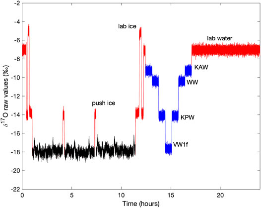
FIGURE 1. Example of uncalibrated (“raw”) δ¹⁷O measurements as reported by the Picarro L2140-i laser spectrometer, for a typical measurement day. Ice core data in black, with laboratory-prepared “push ice” in red and reference waters in blue.

We use two of the four reference waters (e.g., KAW and KPW, as shown in Figure 1) for calibration, reserving the other two (in this case, WW and VW1f) as unknowns or “traps”. The precision and accuracy of the calibration are then estimated, respectively, by the standard deviations of each trap and the mean difference with the known value of each trap. We repeat these calculations to obtain four independent estimates of precision and accuracy (one for each reference water).

We also use an adjusted calibration, based on the difference between the known and estimated values of reference waters used as traps, as follows. For each δ type (i.e., δ¹⁷O, δ¹⁸O, or δD), let X_ref=(x_1,ref,x_2,ref…x_n,ref) be the set of measured “raw” values of reference waters used for calibration, and Y_ref the corresponding known (calibrated against VSMOW-SLAP) values from Table 1. Let X_trap=(x_1,trap,x_2,trap…x_n,trap) be the set of measured “raw” values of reference waters used as traps, and Y_trap the corresponding known calibration values. Obtain the slope, m and intercept, b using

$m=\frac{{{{\displaystyle \sum }}^{\text{}}}_{i=1}^n\left(x_{i,ref}-{\overline{X}}_{ref}\right)\left(y_{i,ref}-{\overline{Y}}_{ref}\right)}{\left(x_{i,ref}-{\overline{X}}_{ref}\right)}(5)$

$b={\overline{Y}}_{ref}-m{\overline{X}}_{ref}(6)$

where $\overline{X},\overline{Y}$ denote means. The calibration equation for a given δ type is,

${\delta }_{calibrated}=m\left({\delta }_{sample,measured}\right)+b(7)$

Equations 5–7 define the simple linear approach. The slope and intercept values are used to obtain estimated values for those reference waters that have been reserved as unknown “traps”:

${\overline{Y}}_{trap,estimated}=m{\overline{X}}_{trap}+b(8)$

The adjustment to the intercept, b, is given by the difference between the estimated trap values Y_{trap,estimated} and their known values from Table 1:

$b_{adjusted}=b-{\overline{Y}}_{trap,known}-{\overline{Y}}_{trap,estimated}(9)$

The adjusted calibration equation for a given δ type is then given by

${\delta }_{calibrated,adjusted}=m\left({\delta }_{sample,measured}\right)+b_{adjusted}(10)$

The simple linear approach (Eq. 7) yields highly reproducible results for δ¹⁸O, δD, and deuterium excess, as previously shown by Jones et al. (2017b), as well as for δ¹⁷O. For Δ¹⁷O, results are significantly improved if the adjusted calibration approach (Eq. 10) is used. The a priori justification for this approach is that the slope of the calibration varies by less than 1%, while the intercept varies by as much as 50%, so that errors in the intercept have a much greater impact on the results. We find that using any combination of reference waters and traps yields essentially indistinguishable results. The final data set is based on the use of the two reference waters KAW and KPW as our primary reference waters and VW1f and WW as the traps. We note that the lowest isotope values in the South Pole core are more negative than the most depleted reference water (VW1f) or standard (SLAP).

In general, we use the reference waters analyzed at the end of a measurement day to calibrate the ice core data from that same day. For measurements of Δ¹⁷O with the L2140-i, it is critical to monitor changes to the currents provided in five channels to the piezoelectric material (lead zirconate titanate, PZT), that is used to vary the length of the laser cavity (Steig et al., 2014). Periodic adjustments to the laser cavity size, which is subject to drift and hysteresis, are made as part of routine instrument operation to achieve laser resonance at the target wavelength. Changes to the PZT values influence the instrument calibration, which can significantly affect Δ¹⁷O if it is not accounted for during calibration of raw measurements to obtain final values on the VSMOW-SLAP scale. We use the PZT values to ensure that calibration reference waters and ice core samples have been measured during the same “calibration window”, as described in Schauer et al. (2016). For example, if there is a change to the ordering of the PZT offset values during a measurement day, we use the reference water values from the previous day.

3 Results

3.1 Instrument Performance

3.1.1 δ¹⁷O, δ¹⁸O, and δD

Assessment of the quality of δ¹⁸O and δD measurements obtained with our CFA system and the L2130-i on the WAIS Divide ice core has been treated previously (Jones et al., 2017b), and the same findings generally apply to our measurements for South Pole on the L2140-i, including the novel meaurement of δ¹⁷O. In this section, we discuss δ¹⁷O, δ¹⁸O, and δD results for the analysis of the South Pole ice core. We discuss the “excess” parameters, d and Δ¹⁷O, in more detail in the next section.

We use three primary methods of assessment: Allan-variance statistics of long measurements of reference waters, reproducibility of reference water values, and reproducibility of replicate ice-core sections.

The Allan variance (Werle, 2011) is given by,

${\sigma }_{Allan}^2\left({\tau }_m\right)=\frac{1}{2m}{\displaystyle \sum }_{j=1}^m{\left({\overline{\delta }}_{j+1}-{\overline{\delta }}_j\right)}^2(11)$

where τ_m is the integration time and δ_j, δ_j+1 are mean isotope values over neighboring time intervals.

We calculate the Allan variance from long (>16 h) continuous measurements of our reference waters, run after each week of ice-core measurements. The measurement set-up is identical to that for the reference-water measurements run daily for shorter time periods. The Allan deviation (σ_Allan, square-root of the Allan variance) establishes the maximum precision and accuracy achievable with the CFA system under ideal operating conditions, as a function of measurement time.

Figure 2 shows the Allan deviation for δ¹⁷O, δ¹⁸O and δD. For integration times as short as 10 s, σ_Allan for δ¹⁷O and δ¹⁸O is <0.1‰ and for δD is <0.3‰. Given our ice-core sampling rate of 2 cm/min, this implies that precision better than these values should be maintained for data averages providing a sampling resolution of less than 0.5 cm (i.e. integration time of 15 s). For longer integration times, higher precision can be achieved; these experiments suggest that limits to precision (indicated by the asymptopic character of the traces, particularly evident for δD, at the longest integration times) are about 0.01‰ for δ¹⁷O and δ¹⁸O, and 0.1‰ for δD. Comparison with the results in Steig et al. (2014) and Schauer et al. (2016) shows that the L2140-i, as used during our sampling campaign for the South Pole ice core, was functioning as well or better than expected from earlier experiments.

FIGURE 2

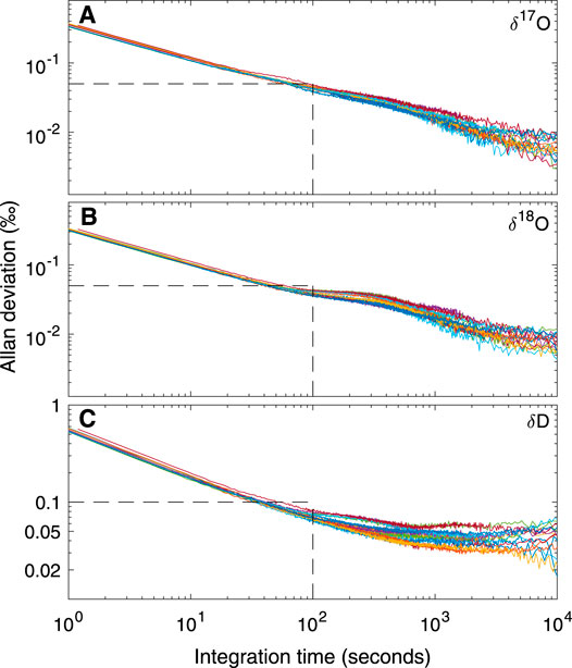
FIGURE 2. Allan deviation for (A)δ¹⁷O (B)δ¹⁸O, and (C)δD from fifteen long reference water measurements using the CFA system. Each color represents a different day of measurements. Dashed lines illustrate that for integration times of 100 s, precision is less than 0.05‰ for δ¹⁷O and δ¹⁸O and <0.1‰ for δD.

Table 2 quantifies the reproducibility of reference waters, where the values shown are for each of the reference waters treated as an unknown “trap”, calibrated (Equations 5–7) with two other reference waters. Values for “precision” are the standard deviation of all measurements for each reference water. “Accuracy” is the mean difference between the calibrated values and the known values. The results show that both precision and accuracy of the reference water measurements is better than 0.05‰ for δ¹⁷O, <0.07‰ for δ¹⁸O, and <0.9‰ for δD. We note that for δD, the Allan-deviation calculations underestimate the reference-water reproducibility by a greater amount than for δ¹⁷O or δ¹⁸O; this suggests greater long term drift for δD than for the other isotope ratios, consistent with the shape of Allan-deviation traces (Figure 2).

TABLE 2

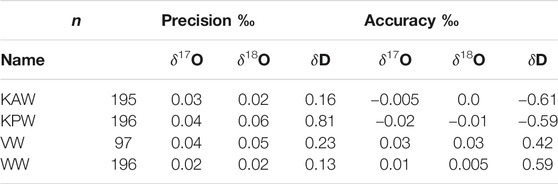
TABLE 2. Precision and accuracy of reference waters measured as unknowns. n = number of independent measurements.

Figure 3 shows the complete VSMOW-SLAP calibrated δ¹⁷O, δ¹⁸O, and δD records as function of depth in the South Pole ice core, along with replicate measurements, averaged to 50 cm for clarity. Table 3 shows the root mean square error (RMS) of the difference between replicates, as a function of depth-averaging interval and approximate integration time, given the routine ice-core melting rate of 2 cm/min. These comparisons provide an effective measure of external precision. External precision is not as good as the internal precision implied by reference water calculations discussed above, generally being about twice as large for equivalent time averaging. RMS error for δ¹⁸O for 50 cm averages, equivalent to an integration time of ∼1,500 s is 0.1‰ (Table 3), while the typical standard deviation of reference water values treated as unknowns is 0.05‰ (Table 2) (recall that reference waters were generally measured for 2000 s). This is to be expected, since the reference-water measurements involve vaporization from liquid water under very steady conditions, while the ice-core measurements involve additional variables, such as subtle variations in flow rate as a function of ice density. The reproduciblity, even at very high spatial resolution, is still very good. For example, the value for δD of 1.3‰ for 0.5 cm averages, and <<1‰ for longer averages, is comparable to the precision typically reported for ice core δD on the basis of comparatively low-resolution discrete measurements (e.g., Masson-Delmotte et al., 2005).

FIGURE 3

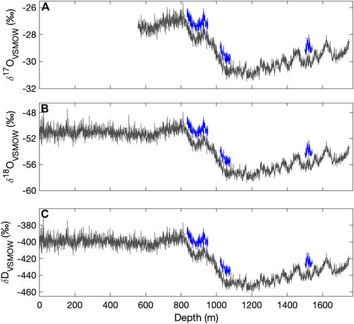
FIGURE 3. Calibrated (A)δ¹⁷O (B)δ¹⁸O and (C)δD for the South Pole ice core (SPC14), from continuous-flow measurements with the Picarro L2140-i (the upper section (to 556 m) was analyzed only with the L2130-i). Data are shown as 50-cm averages, plotted at their mid-point depth. Replicate data (blue) are offset vertically by 1, 2, and 16‰ for δ¹⁷O, δ¹⁸O and δD, respectively.

TABLE 3

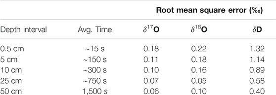
TABLE 3. Root mean square difference between primary and replicate ice core samples, as a function of depth-averaging window. “Avg. time” is approximate time-average corresponding to each depth interval.

3.1.2 Deuterium Excess and ¹⁷O Excess

We consider the same metrics as above for d and Δ¹⁷O. As shown in Figure 4, the Allan deviation for d is similar to that for δD, with values <0.5‰ obtained even for high-frequency measurements. For Δ¹⁷O, longer intergrations are required, with averages >10³s necessary for routinely obtaining precision better than 0.01‰. Consistent with this, the reproducibility of “trap” reference water averages is 0.009–0.011‰, except for the extremely depleted Vostok water (VW1f), which has standard deviation of 0.016‰ Table 4. The relatively poor Δ¹⁷O reproducibility may result from the extrapolation, rather than interpolation between two reference waters.

FIGURE 4

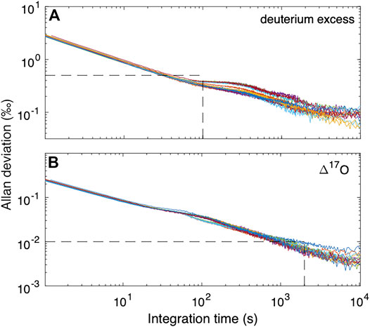
FIGURE 4. Allan deviation for (A)d (deuterium excess) and (B) Δ¹⁷O from reference water measurements using the CFA system. Dashed lines in (A) show that for integration times of 100 s, precision for d is less than 0.5‰. For Δ¹⁷O, longer measurement times are required. Vertical dashed line in (B) is at 2000 s, corresponding to Δ¹⁷O precision <0.01‰ (10 per meg).

TABLE 4

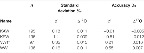
TABLE 4. Precision and accuracy of deuterium excess and ¹⁷O excess for reference waters measured as unknowns. n = number of independent measurements.

Figure 5 shows the full d and Δ¹⁷O data from the South Pole ice core as 1-m averages for clarity, along with replicate continuous-flow data as in Figure 3. Also shown in Figure 5 are 1 m averages of the 1/2 m discrete replicate samples measured with the L2140-i and autosampler, following Schauer et al. (2016). As shown in Table 5, the resulting comparison indicates acceptable deuterium excess reproducibility (<1‰) at depth-averages of a few cm or less. For Δ¹⁷O, averages of >10³s are required for reproducibility better than <0.01‰.

FIGURE 5

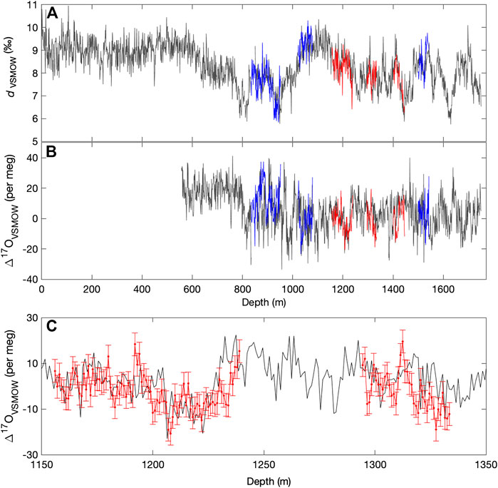
FIGURE 5. (A) Deuterium excess and (B) Δ¹⁷O for the South Pole ice core (SPC14), from continuous-flow measurements with the Picarro L2140-i, calibrated with Eq. 10. Main data set in gray, with replicate continuous-flow (dark blue) and discrete data (red). (C) shows an enlarged section of discretely measured replicate data, with 1 standard deviation (10 per meg) error bars. All data are shown as 100 cm averages.

TABLE 5

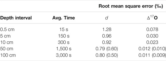
TABLE 5. Root mean square error for deuterium excess (d) and ¹⁷O excess (Δ¹⁷O) between primary and replicate ice core samples, as a function of depth-averaging window. Values in parentheses are for the measurements on discrete 1/2 m samples (red data in Figure 5). “Avg. time” is approximate time-average corresponding to each depth interval.

3.1.3 Sensitivity to Calibration Method, and Comparison Between L2130-i and L2140-i

As described above, we use a modification to the simple linear calibration, in which the values of two “trap” reference waters are used to adjust the calibration intercept. With this adjustment, reproducibility of Δ¹⁷O, as evaluated by replicate measurements, is improved, and the total variance in the data is reduced, as illustrated in Figure 6. The size of the adjustment does not depend on the mean isotope values. We do note that the replicate data (Figure 5) suggest that the errors are not truly random – that is, there is evidence of systematic offsets, such as between ∼1,330 and 1,340 depth, which our calibration procedure does not fully address. The calibration method does not, however, influence the other δ values or d appreciably, though the resulting data sets are slightly different, as shown in Figure 7, which compares δ¹⁸O and d measurements obtained on the L2130-i without the adjusted calibration, and on the L2140-i with and without the adjusted calibration.

FIGURE 6

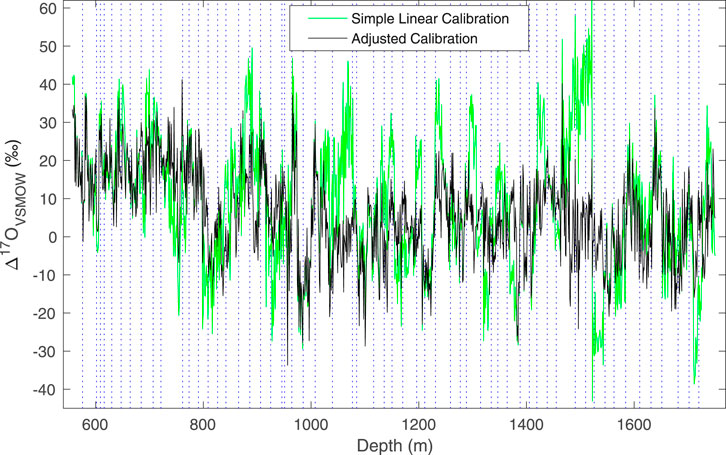
FIGURE 6. Comparison of 100 cm average Δ¹⁷O data for the South Pole ice core, calibrated with a simple linear calibration (green, Eq. 7) with two reference waters, and an adjusted calibration (gray, Eq. 10) using four reference waters. Note the increased variance and abrupt transitions in the un-adjusted data. Dashed vertical lines define the boundary between different analysis days.

FIGURE 7

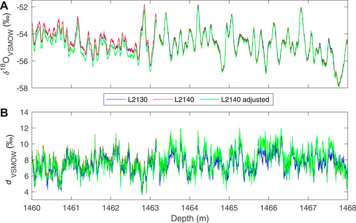
FIGURE 7. Comparison of (A)δ¹⁸O and (B) deuterium excess for the South Pole ice core (SPC14) for a short section of the core at high (0.5 cm) resolution, from two different instruments. The data from the Picarro L2130-i (blue) are calibrated with simple two-point calibration (Eq. 7). Data from the Picarro L2140-i are shown with both the simple (red) and adjusted calibration (Eq. 10 (green)).

The differences between the different instruments and different calibrations, up to ∼0.1‰ in δ¹⁸O and ∼0.3‰ in d are not likely to be important for any practical use (i.e., for paleoclimate interpretation) because they are much smaller than the climate-related variability. Nevertheless, the high-resolution, δD and d data obtained with the L2130-i are in general slightly less noisy (regardless of the calibration used). This has been noted in previous work and can be attributed to differences in the spectroscopy of the two instruments (Steig et al., 2014). Subtle differences between the data sets could lead to confusion if they were used without attention to the details. For example, calculating Δ¹⁷O using δ¹⁸O from the L2130-i and δ¹⁷O from the L2140-i would create significant artifacts, as would calculating deuterium excess from two different instruments. We recommend using the L2130-i for δ¹⁸O and δD where possible. We provide an equivalent “L2130” measure of δ¹⁷O, using the definition of Δ¹⁷O:

${\delta }^{17}{O}_{VSMOW,\left(\text{L}2130\right)}=exp[{\text{Δ}}^{17}{O}_{VSMOW,\left(\text{L}2140\right)}+0.528\left(ln({\delta }^{18}{O}_{VSMOW,L2130}+1)\right]-1(12)$

where the subscripts indicate from which instrument the data are obtained. This results in a single set of mutually consistent, high resolution δ¹⁷O, δ¹⁸O and δD data for the South Pole ice core, from which Δ¹⁷O and d may be calculated, identical to that obtained from the L2140-i and L2130-i, respectively. This final data set is used in the Discussion section which follows. We emphasize that in practice, either instrument provides excellent data that are indistuishable for any practical purpose.

4 Discussion

4.1 Continuous-Flow Measurements of the Complete Oxygen and Hydrogen Isotope Ratios of Water

Continuous-flow analyses of the isotopic composition of H₂O in ice cores have advanced significantly since the early, discontinous measurements of discrete samples pioneered by Johnsen et al. (1972), Dansgaard et al. (1982), and others. The development of laser spectrometers (Crosson, 2008) has reduced the use of mass spectrometry, and allowed the development of continuous-flow analysis of ice-core water isotopes (Gkinis et al., 2010). This method has been successful both with Picarro cavity ring-down spectroscopy (Gkinis et al., 2010; Gkinis et al., 2011; Maselli et al., 2013; Jones et al., 2017b; Hughes et al., 2020) as we use here, as well as off-axis integrated cavity output spectroscopy (Los Gatos Instruments) (Emanuelsson et al., 2015). With the inclusion of δ¹⁷O and Δ¹⁷O, our results represents a further advance of this earlier work.

In general, the analytical error of δ¹⁸O and δD measurements on ice cores is much smaller than the signal being measured. Our results show that the same is true for δ¹⁷O. For example, RMS errors for replicates (our most conservative estimate of precision) are <0.1, <0.9, and <0.1‰, respectively, for 10 cm averages of δ¹⁸O, δD, and δ¹⁷O. For most of the length of the South Pole ice core, 10 cm corresponds to just a few years. Interannual, decadal and centennial variations of δ¹⁸O are typically 1–2‰ (e.g., Steig et al., 2013); variability in δ¹⁷O is about half that of δ¹⁸O, and variability in δD is about eight times greater. Millennial and glacial-interglacial changes are up to an order of magnitude larger (e.g., Grootes et al., 1993; EPICA Community Members, 2006; WAIS Divide Project Members, 2015). A measure of the signal to noise ratio (amplitude of the natural variablity over the RMS error) is therefore between 10 and 100 for all three types of δ measurement. This suggests that δ¹⁷O, like δ¹⁸O and δD, can be considered a routine measurement. Indeed, the measurement of δ¹⁷O by CFA poses no particular challenge that has not already been addressed in previous work for δ¹⁸O and δD. We would expect similar results with other available instruments such as the Los Gatos isotopic water analyzer (Berman et al., 2013) or other commerial or non-commerical instruments of similar design to the Picarro L2140-i used here.

Natural variations in d in ice cores are typically smaller than those in δ¹⁸O, while precision, about 0.5–1‰, is similar to that for δD. For example, millennial-scale variabilty in d in Antarctic ice cores is only about 1–2‰ (Markle et al., 2017); in contrast δD varies by 10–20‰ on the same timescale. Ice core d data is thus comparatively “noisy”, and relatively long averaging windows are typically required. Similar to d, the signal to noise ratio is low for Δ¹⁷O. For our measurements on the South Pole ice core, depth averages of at least 50 cm are needed to reduce the analytical error to 0.01‰ (10 per meg). The best mass-spectrometry measurements of Δ¹⁷O have reported precisions of as little as 4 per meg, though this is generally the standard error of multiple replicate measurements on discrete samples (e.g., Barkan and Luz, 2007; Schoenemann et al., 2013); more typical reproducibility is 6–8 per meg (Landais et al., 2008; Schoenemann et al., 2014; Landais et al., 2017). Previous work shows that millennial variations in Greenland Δ¹⁷O are of order 30 per meg (Guillevic et al., 2014), and our South Pole ice core record shows variations of the same magnitude. Considering these timescales, the signal to noise ratio of our data for 50 cm averages is therefore about ∼3, similar to that for d. In the South Pole core, 50 cm averages corresponds to a time resolution of only a few decades, so longer averages can be used to further reduce the noise when examining variability on longer timescales. For applications where the very highest resolution is sought (e.g., resolving the annual cycle, or obtaining measurements at high temporal resolution in ice that has been significantly thinned, such as near the bed of an ice sheet), continuous-flow techniques for Δ¹⁷O may be less valuable, and discrete measurements, while labor intensive, are still warranted.

In summary, our results show that measurements of ice-core δ¹⁷O and Δ¹⁷O can be achieved by continous-flow methods that are competitive, in terms of the signal-to-noise, with traditional δ¹⁸O and deuterium excess measurements, respectively. Our results for the South Pole ice core, while somewhat lower quality than the best-possible mass-spectrometery or discrete laser-spectroscopy measurements, provide useful information for the investigation of climate variability and other applications.

4.2 Isotope Records From the South Pole Ice Core

We now consider the complete water-isotope records from the South Pole ice core, and provide two examples of the use of these data. One important application of high-resolution isotope data is the calculation of the water-isotope diffusion length. As dry snow densifies to firn and ice, water vapor diffuses through interconnected pathways, smoothing the original isotope signal (Johnsen et al., 1972; Whillans and Grootes, 1985; Cuffey and Steig, 1998). The diffusion length, σ, is given by the solution to the differential equation (Johnsen, 1977)

$\frac{d{\sigma }^2}{2dt}-\dot{\mathit{ϵ}}\left(t\right){\sigma }^2=D_i^{\text{*}}\left(t\right)(13)$

where t is time, ϵ˙ is the vertical strain rate (due to compression of the firn, and dynamic thinning of the ice), and D_i^*(t) is the effective diffusivity in the firn or ice of isotopic species i. Measurements of the diffusion length in ice core records can be used, in combination with models of the firn-densification process, as an independent measure of paleotemperature (Johnsen et al., 2000; Simonsen et al., 2011; Gkinis et al., 2014; van der Wel et al., 2015), and for correction of high-frequency paleoclimate signals (Jones et al., 2018). Because of the dependence on strain, diffusion-length measurements also provide information on ice thinning (Gkinis et al., 2014). In Figure 8 we show the diffusion length measurements, calculated using the spectral analysis-based method described in Kahle et al. (2018). Of particular interest is that the diffusion length for δ¹⁷O is systematically greater than that for δ¹⁸O, which is again greater than that for δD, as expected from theory. Johnsen et al. (2000) and van der Wel et al. (2015) have suggested that using the ratio (e.g. σ17/σD) or difference (e.g. σ17−σD) of diffusion lengths for different isotopologues can constrain firn temperature because temperature is the stronger control on those differences or ratios than on individual diffusion lengths. However, the small differences between diffusion lengths has made such calculations unsuccessful in practice (Holme et al., 2018). In this respect, the greater magnitude of the difference σ17−σD than σ18−σD could be advantageous, as Simonsen et al. (2011) have suggested. In principle these data could be also used to independently verify laboratory-based measurements of isotopic diffusivity, which remain uncertain (Hellmann and Harvey, 2020).

FIGURE 8

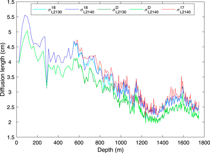
FIGURE 8. Diffusion lengths, σ, from five different high-resolution isotope-ratio measurements from the South Pole ice core, determined using the methods described in Kahle et al. (2018). The superscripts 17, 18, D refer to δ¹⁷O, δ¹⁸O, δD, and the subscripts L2130, L2140 to the instrument used. All calculations were made on 250-year windows of the 0.5 cm high-resolution calibrated data, using the ice timescale of (Winski et al., 2019). σ from δ¹⁷O recalculated for the L2130 (Eq. 12, not shown) is indistinguishable from the original data.

Figure 9 shows the δ¹⁸O, deuterium excess and Δ¹⁷O, averaged to 100-years resolution, from the South Pole ice core, on the timescale from Winski et al. (2019). We include both the conventional linear deuterium excess (d, Eq. 2) and the logarithmic form (d_ln, Eq. 3). For the Holocene (most recent ∼12,000 years), 100 years resolution is equivalent to about 5 m averages; for older portions of the core, snow accumulation rates were lower and 100 years corresponds to about 2 m averages.

FIGURE 9

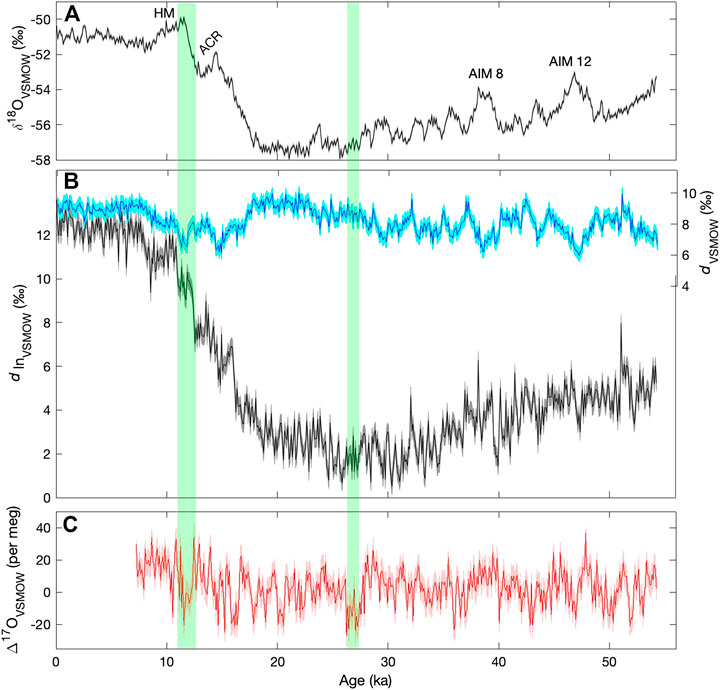
FIGURE 9. Water isotope time series from the South Pole ice core, shown at a resolution of 100 years (A)δ¹⁸O (B), d (light blue) and d_ln (dark blue) (C), Δ¹⁷O. Shading shows 2 standard deviation analytical uncertainties determined from replicate measurements. Labels in the top panel show the Holocene maximum (HM), the Antarctic Cold Reversal (ACR), and the two most prominent Antarctic Isotope Maximum (AIM) events. Green vertical bars highlight features in the Δ¹⁷O record referred to in the text.

The δ¹⁸O time series in Figure 9 shows the typical pattern of variation seen in other ice cores from East Antarctica, with an early Holocene maximum (HM), the “Antarctic Cold Reversal” (ACR) between 14.7 ka and 13.0 ka (ka = thousands of years before present), and the Antarctic Isotope Maximum (AIM) events, the most prominent two of which are labeled. Such features provide a useful reference, when discussing the significance of the novel deuterium excess and Δ¹⁷O results.

Of particular interest is the relationship between Δ¹⁷O and d_ln, and d. The traditional formulation for deuterium excess, d, is subject to artifacts resulting from the linear approximation to non-linear processes. The d_ln calculation is intended to be more faithful to the physics of the system (Uemura et al., 2012); this also motivates the non-linear definition of Δ¹⁷O (Landais et al., 2008). Consistent with this, 100-year average Δ¹⁷O is better correlated with d_ln (r = 0.3) than with d (r = −0.15). However, neither correlation is statistically significant at millennial frequencies, after accounting for autocorrelation.

Markle et al. (2017) showed that in the WAIS Divide ice core, d_ln is in phase with δ¹⁸O for long timescales, but shows abrupt transitions that correspond to the abrupt changes recorded in Greenland ice cores–the Dansgaard-Oeschger (D-O) events. Markle et al. (2017) showed that d_ln variations can be explained as a combination of slowly varying sea surface temperatures (SST), in phase with Antarctic δ¹⁸O, and faster-varying atmospheric shifts of moisture sources for Antarctic precipitation, in phase with D-O events. Later work verified the same relationships for additional Antarctic ice cores (Buizert et al., 2018; Svensson et al., 2020). A key element of this argument is that millennial scale changes in Antarctic d_ln are associated with changes in the evaporative conditions at the ocean surface–both SST and humidity–which affect the initial d_ln of water vapor over the ocean surface at the point of evaporation. Δ¹⁷O, like d_ln, is sensitive to humidity variations, but not directly to SST (Landais et al., 2008). We would therefore expect to see similarities between d_ln and Δ¹⁷O at millennial periods, if humidity variations dominate the d_ln signal, but less agreement if SST variations dominate. As already noted, the correlation between these variables is not significant on millennial timescales. Furthermore, the relative scaling between d_ln and Δ¹⁷O is inconsistent with an attribution to humidity variations. For example, the millennial-scale variations in d_ln we observe in the South Pole ice core have an amplitude of about 1‰, while the Δ¹⁷O amplitude is about 0.01‰ (10 per meg), where we estimate the amplitude from the standard deviation of highpass filtered data, with a 5,000-year cut-off period. A change of 10 per meg in Δ¹⁷O could be attributed to a ∼20% change in humidity at the ocean surface; all else being equal this would also cause a change of about 10‰ in d_ln – that is, variability about an order of magnitude larger than we observe — based on the data in Uemura et al. (2008; 2010). This suggests that the attribution of d_ln variations to the SST of the moisture sources for Antarctic precipitation (Markle et al., 2017) is more consistent with the evidence. However, this leaves the millennial-scale Δ¹⁷O variations unexplained. We note that these findings do not preclude a significant role for humidity in explaining Δ¹⁷O variations in Greenland ice cores (Guillevic et al., 2014), in which all these variables are more highly correlated with one another than they are in the South Pole record.

Finally, we note two interesting features of the Δ¹⁷O time series that warrant further study. There is a significant drop in Δ¹⁷O between 12.8 ka and 11.7 ka, corresponding to the Northern Hemisphere Younger Dryas, and also characterized by a rapid increase in d_ln, and a more gradual increase in δ¹⁸O that defines the end of the Antarctic Cold Reversal. This is one of the few features in the record where all water-isotope variables show correlated changes. In contrast, another prominent feature in Δ¹⁷O, an abrupt drop in values at about 28 ka, has no obvious counterpart in d_ln or δ¹⁸O (This event occurs at about 1200 m depth in the South Pole ice core, and is verified by triplicate measurements — see Figure 5). Interpretation of these relationships is not straightforward and would likely benefit from isotope-modeling studies that incorporate the complete set of water-isotope variables.

5 Conclusion

In this study, we describe the use of a continuous-flow analysis system to measure the complete set of water isotopologues on ice cores, yielding simultaneous measurements of δD, δ¹⁸O, and δ¹⁷O, as well as the “excess” parameters, d, d_ln, and Δ¹⁷O. The inclusion of δ¹⁷O and Δ¹⁷O in CFA measurements marks a significant advance. We show that, using laser spectroscopy, precise CFA measurements of δ¹⁷O are as straightforward as the more conventional δD and δ¹⁸O. While Δ¹⁷O measurements remain challenging, requiring careful attention to instrument operating conditions, results can be obtained with CFA that are competitive with discrete laser or IRMS measurements.

We produced a complete 54,000-year record of δD, δ¹⁸O, d, and d_ln on an ice core from the South Pole, as well as a ∼50,000-year record of δ¹⁷O and Δ¹⁷O. The practical resolution of the δD, δ¹⁸O and δ¹⁷O time series is 0.5 cm, providing a rich data set for exploring high-frequency climate variabilty, and studies of diffusion. The effective resolution of Δ¹⁷O is limited to 50 cm or greater, because of the long averaging times required for precise measurements. Despite this, the comparatively large natural variations in Δ¹⁷O on millennial timescales means that the signal-to-noise ratio for Δ¹⁷O is similar to that for deuterium excess, which has long been used in ice core studies. An initial analysis of the results suggests promise for disentangling the competing effects of temperature, humidity, and other factors, in controlling the variations in both these isotopic variables.

Data Availability Statement

The datasets presented in this study can be found at the US Antarctic Data Center: https://www.usap-dc.org/view/dataset/601429 and https://www.usap-dc.org/view/dataset/601239.

Author Contributions

ES and JW conceived the project. ES wrote the paper, prepared figures and conducted the statistical analyses. TJ, EK, AS, VM, and BV measured the ice core sample and processed the raw data. LD helped with the analysis of the data. All authors contributed to editing the final manuscript.

Funding

This work was funded by the U.S. National Science Foundation, under Office of Polar Program awards 1443105, 1443328 and 1141839.

Conflict of Interest

The authors declare that the research was conducted in the absence of any commercial or financial relationships that could be construed as a potential conflict of interest.

Acknowledgments

We thank the following University of Colorado and University of Washington graduate and undergraduate students for their help in sampling and analyzing the South Pole ice core: A. Hughes, W. Skorski, S. Salzwedel, B. Oliver, C. Czarnecki, A. Servettaz, N. Tanski, David Pasquale, Z. Brown, Ben Sinnet, S. L. Tetreau, B. Chase, J. Davis, R. McGehee, H. Williamson, O. Van de Graaf, A Kessenich, C. Vanderheyden. We thank M. Aydin, M. Twickler and J. Souney for their work administering the South Pole ice core project, the U.S. Ice Drilling team at the University of Wisconsin, the NSF Ice Core Facility, the 109th New York Air National Guard and the U.S. Antarctic Program for the collection, transport, processing, and storage of the core. We also thank the reviewers for their constructive reviews, which led to improvements to the original version of this paper.

References

Barkan, E., and Luz, B. (2007). Diffusivity fractionations of H₂¹⁶O/H₂¹⁷O and H₂¹⁶O/H₂¹⁸O in air and their implications for isotope hydrology. Rapid Commun. Mass. Spectrom. 21, 2999–3005. doi:10.1002/rcm.3180

PubMed Abstract | CrossRef Full Text | Google Scholar

Barkan, E., and Luz, B. (2005). High precision measurements of¹⁷O/¹⁶O and ¹⁸O/¹⁶O ratios in H₂O. Rapid Commun. Mass. Spectrom. 19, 3737–3742. doi:10.1002/rcm.2250

PubMed Abstract | CrossRef Full Text | Google Scholar

Berman, E. S., Levin, N., Landais, A., Li, S., and Owano, T. (2013). Measurement of δ¹⁸O, δ¹⁷O, and ¹⁷O-excess in water by off-axis integrated cavity output spectroscopy and isotope ratio mass spectrometry. Anal. Chem. 85, 10392. doi:10.1021/ac402366t

PubMed Abstract | CrossRef Full Text | Google Scholar

Bigler, M., Svensson, A., Kettner, E., Vallelonga, P., Nielsen, M. E., and Steffensen, J. P. (2011). Optimization of high-resolution continuous flow analysis for transient climate signals in ice cores. Environ. Sci. Tech. 45, 4483–4489. doi:10.1021/es200118j

CrossRef Full Text | Google Scholar

Buizert, C., Sigl, M., Severi, M., Markle, B. R., Wettstein, J. J., McConnell, J. R., et al. (2018). Abrupt ice-age shifts in southern westerly winds and antarctic climate forced from the north. Nature 563, 681–685. doi:10.1038/s41586-018-0727-5

PubMed Abstract | CrossRef Full Text | Google Scholar

Casey, K. A., Fudge, T. J., Neumann, T. A., Steig, E. J., Cavitte, M. G. P., and Blankenship, D. D. (2014). The 1500 m South Pole ice core: recovering a 40 ka environmental record. Ann. Glaciol. 55, 137–146. doi:10.3189/2014aog68a016

CrossRef Full Text | Google Scholar

Coplen, T. B. (1988). Normalization of oxygen and hydrogen isotope data. Chem. Geology. Isotope Geosci. sec. 72, 293–297. doi:10.1016/0168-9622(88)90042-5

CrossRef Full Text | Google Scholar

Coplen, T. B., Wildman, J. D., and Chen, J. (1991). Improvements in the gaseous hydrogen-water equilibration technique for hydrogen isotope-ratio analysis. Anal. Chem. 63, 910–912. doi:10.1021/ac00009a014

CrossRef Full Text | Google Scholar

Crosson, E. R. (2008). A cavity ring-down analyzer for measuring atmospheric levels of methane, carbon dioxide, and water vapor. Appl. Phys. B 92, 403–408. doi:10.1007/s00340-008-3135-y

CrossRef Full Text | Google Scholar

Cuffey, K. M., and Steig, E. J. (1998). Isotopic diffusion in polar firn: implications for interpretation of seasonal climate parameters in ice-core records, with emphasis on central Greenland. J. Glaciol. 44, 273–284. doi:10.3189/s0022143000002616

CrossRef Full Text | Google Scholar

Dansgaard, W., Clausen, H., Gundestrup, N., Hammer, C., Johnsen, S., Kristinsdottir, P., et al. (1982). A new Greenland deep ice core. Science 218, 1273–1277. doi:10.1126/science.218.4579.1273

PubMed Abstract | CrossRef Full Text | Google Scholar

Dansgaard, W. (1964). Stable isotopes in precipitation. Tellus 16, 436–468. doi:10.3402/tellusa.v16i4.8993

CrossRef Full Text | Google Scholar

Dütsch, M., Blossey, P. N., Steig, E. J., and Nusbaumer, J. M. (2019). Nonequilibrium fractionation during ice cloud formation in iCAM5: evaluating the common parameterization of supersaturation as a linear function of temperature. J. Adv. Model. Earth Syst. 11, 3777–3793. doi:10.1029/2019MS001764

CrossRef Full Text | Google Scholar

Emanuelsson, B. D., Baisden, W. T., Bertler, N. A. N., Keller, E. D., and Gkinis, V. (2015). High-resolution continuous-flow analysis setup for water isotopic measurement from ice cores using laser spectroscopy. Atmos. Meas. Tech. 8, 2869–2883. doi:10.5194/amt-8-2869-2015

CrossRef Full Text | Google Scholar

EPICA Community Members (2006). One-to-one coupling of glacial climate variability in Greenland and Antarctica. Nature 444, 195–198. doi:10.1038/nature05301

PubMed Abstract | CrossRef Full Text | Google Scholar

Epifanio, J. A., Brook, E. J., Buizert, C., Edwards, J. S., Sowers, T. A., Kahle, E. C., et al. (2020). The SP19 chronology for the South Pole Ice Core - Part 2: gas chronology, Δage, and smoothing of atmospheric records. Clim. Past 16, 2431–2444. doi:10.5194/cp-16-2431-2020

CrossRef Full Text | Google Scholar

Epstein, S., and Mayeda, T. (1953). Variation of O18 content of waters from natural sources. Geochimica et Cosmochimica Acta 4, 213–224. doi:10.1016/0016-7037(53)90051-9

CrossRef Full Text | Google Scholar

Gkinis, V., Popp, T. J., Johnsen, S. J., and Blunier, T. (2010). A continuous stream flash evaporator for the calibration of an IR cavity ring-down spectrometer for the isotopic analysis of water. Isotopes Environ. Health Stud. 46, 463–475. doi:10.1080/10256016.2010.538052

PubMed Abstract | CrossRef Full Text | Google Scholar

Gkinis, V., Popp, T. J., Blunier, T., Bigler, M., Schüpbach, S., Kettner, E., et al. (2011). Water isotopic ratios from a continuously melted ice core sample. Atmos. Meas. Tech. 4, 2531–2542. doi:10.5194/amt-4-2531-2011

PubMed Abstract | CrossRef Full Text | Google Scholar

Gkinis, V., Simonsen, S. B., Buchardt, S. L., White, J. W. C., and Vinther, B. M. (2014). Water isotope diffusion rates from the NorthGRIP ice core for the last 16,000 years - glaciological and paleoclimatic implications. Earth Planet. Sci. Lett. 405, 132–141. doi:10.1016/j.epsl.2014.08.022

CrossRef Full Text | Google Scholar

Gonfiantini, R. (1978). Standards for stable isotope measurements in natural compounds. Nature 271, 534–536. doi:10.1038/271534a0

CrossRef Full Text | Google Scholar

Grootes, P. M., Stuiver, M., White, J. W. C., Johnsen, S., and Jouzel, J. (1993). Comparison of oxygen isotope records from the GISP2 and GRIP Greenland ice cores. Nature 366, 552–554. doi:10.1038/366552a0

CrossRef Full Text | Google Scholar

Guillevic, M., Bazin, L., Landais, A., Stowasser, C., Masson-Delmotte, V., Blunier, T., et al. (2014). Evidence for a three-phase sequence during Heinrich Stadial 4 using a multiproxy approach based on Greenland ice core records. Clim. Past 10, 2115–2133. doi:10.5194/cp-10-2115-2014

CrossRef Full Text | Google Scholar

Hellmann, R., and Harvey, A. H. (2020). First‐principles diffusivity ratios for kinetic isotope fractionation of water in air. Geophys. Res. Lett. 47, e2020GL089999. doi:10.1029/2020GL089999

CrossRef Full Text | Google Scholar

Holme, C., Gkinis, V., and Vinther, B. M. (2018). Molecular diffusion of stable water isotopes in polar firn as a proxy for past temperatures. Geochimica et Cosmochimica Acta 225, 128–145. doi:10.1016/j.gca.2018.01.015

CrossRef Full Text | Google Scholar

Hughes, A. G., Jones, T. R., Vinther, B. M., Gkinis, V., Stevens, C. M., Morris, V., et al. (2020). High-frequency climate variability in the Holocene from a coastal-dome ice core in east-central Greenland. Clim. Past 16, 1369–1386. doi:10.5194/cp-16-1369-2020

CrossRef Full Text | Google Scholar

Johnsen, S. J., Clausen, H. B., Cuffey, K. M., Hoffmann, G., Schwander, J., and Creyts, T. (2000). “Diffusion of stable isotopes in polar firn and ice. the isotope effect in firn diffusion,” in Physics of ice core records. Editor T. Hondoh (Sapporo: Hokkaido University Press), 121–140.

Google Scholar

Johnsen, S. J., Dansgaard, W., Clausen, H. B., and Langway, C. C. (1972). Oxygen isotope profiles through the Antarctic and Greenland ice sheets. Nature 235, 429–434. doi:10.1038/235429a0

CrossRef Full Text | Google Scholar

Johnsen, S. J., Dansgaard, W., and White, J. W. C. (1989). The origin of Arctic precipitation under present and glacial conditions. Tellus 41B, 452–468. doi:10.1111/j.1600-0889.1989.tb00321.x

CrossRef Full Text | Google Scholar

Johnsen, S. J. (1977). Stable isotope homogenization of polar firn and ice. Proceedings of Symposium on Isotopes and Impurities in Snow and Ice, IAHS-AISH Public. 188, 210–219.

Google Scholar

Johnson, J. A., Kuhl, T., Boeckmann, G., Gibson, C., Jetson, J., Meulemans, Z., et al. (2020). Drilling operations for the South Pole Ice core (SPICEcore) project. Ann. Glaciology. doi:10.1017/aog.2020.64

CrossRef Full Text | Google Scholar

Jones, T. R., Roberts, W. H. G., Steig, E. J., Cuffey, K. M., Markle, B. R., and White, J. W. C. (2018). Southern hemisphere climate variability forced by Northern Hemisphere ice-sheet topography. Nature 554, 351–355. doi:10.1038/nature24669

PubMed Abstract | CrossRef Full Text | Google Scholar

Jones, T. R., Cuffey, K. M., White, J. W. C., Steig, E. J., Buizert, C., Markle, B. R., et al. (2017a). Water isotope diffusion in the WAIS Divide ice core during the Holocene and last glacial. J. Geophys. Res. Earth Surf. 122, 290–309. doi:10.1002/2016JF003938

CrossRef Full Text | Google Scholar

Jones, T. R., White, J. W. C., Steig, E. J., Vaughn, B. H., Morris, V., Gkinis, V., et al. (2017b). Improved methodologies for continuous-flow analysis of stable water isotopes in ice cores. Atmos. Meas. Tech. 10, 617–632. doi:10.5194/amt-10-617-2017

CrossRef Full Text | Google Scholar

Jouzel, J., Alley, R. B., Cuffey, K. M., Dansgaard, W., Grootes, P., Hoffmann, G., et al. (1997). Validity of the temperature reconstruction from water isotopes in ice cores. J. Geophys. Res. 102, 26471–26487. doi:10.1029/97jc01283

CrossRef Full Text | Google Scholar

Jouzel, J., and Merlivat, L. (1984). Deuterium and oxygen 18 in precipitation: modeling of the isotopic effects during snow formation. J. Geophys. Res. 89, 11749–11759. doi:10.1029/jd089id07p11749

CrossRef Full Text | Google Scholar

Jouzel, J., Stiévenard, M., Johnsen, S. J., Landais, A., Masson-Delmotte, V., Sveinbjornsdottir, A., et al. (2007). The GRIP deuterium-excess record. Quat. Sci. Rev. 26, 1–17. doi:10.1016/j.quascirev.2006.07.015

CrossRef Full Text | Google Scholar

Kahle, E. C., Holme, C., Jones, T. R., Gkinis, V., and Steig, E. J. (2018). A generalized approach to estimating diffusion length of stable water isotopes from ice-core data. J. Geophys. Res. Earth Surf. 123, 2377–2391. doi:10.1029/2018JF004764

CrossRef Full Text | Google Scholar

Kaseke, K. F., Wang, L., and Seely, M. K. (2017). Nonrainfall water origins and formation mechanisms. Sci. Adv. 3, e1603131. doi:10.1126/sciadv.1603131

PubMed Abstract | CrossRef Full Text | Google Scholar

Kerstel, E. R. T., van Trigt, R., Reuss, J., Meijer, H. A. J., and Meijer, H. A. J. (1999). Simultaneous determination of the ²H/¹H, ¹⁷O/¹⁶O, and¹⁸O/¹⁶O isotope abundance ratios in water by means of laser spectrometry. Anal. Chem. 71, 5297–5303. doi:10.1021/ac990621e

PubMed Abstract | CrossRef Full Text | Google Scholar

Landais, A., Barkan, E., and Luz, B. (2008). Record of δ¹⁸O and ¹⁷O‐excess in ice from Vostok Antarctica during the last 150,000 years. Geophys. Res. Lett. 35, L02709. doi:10.1029/2007GL032096

CrossRef Full Text | Google Scholar

Landais, A., Casado, M., Prié, F., Magand, O., Arnaud, L., Ekaykin, A., et al. (2017). Surface studies of water isotopes in Antarctica for quantitative interpretation of deep ice core data. Comptes Rendus Geosci. 349, 139–150. doi:10.1016/j.crte.2017.05.003

CrossRef Full Text | Google Scholar

Markle, B. R., Steig, E. J., Buizert, C., Schoenemann, S. W., Bitz, C. M., Fudge, T. J., et al. (2017). Global atmospheric teleconnections during Dansgaard-Oeschger events. Nat. Geosci 10, 36–40. doi:10.1038/ngeo2848

CrossRef Full Text | Google Scholar

Maselli, O. J., Fritzsche, D., Layman, L., McConnell, J. R., and Meyer, H. (2013). Comparison of water isotope-ratio determinations using two cavity ring-down instruments and classical mass spectrometry in continuous ice-core analysis. Isotopes Environ. Health Stud. 49, 387–398. doi:10.1080/10256016.2013.781598.PMID:23713832

PubMed Abstract | CrossRef Full Text | Google Scholar

Masson-Delmotte, V., Jouzel, J., Landais, A., Stievenard, M., Johnsen, S. J., White, J. W., et al. (2005). Grip deuterium excess reveals rapid and orbital-scale changes in Greenland moisture origin. Science 309, 118–121. doi:10.1126/science.1108575

PubMed Abstract | CrossRef Full Text | Google Scholar

Merlivat, L., and Jouzel, J. (1979). Global climatic interpretation of the deuterium-oxygen 18 relationship for precipitation. J. Geophys. Res. 84 (C8), 5029–5033. doi:10.1029/jc084ic08p05029

CrossRef Full Text | Google Scholar

Petit, J. R., White, J. W. C., Young, N. W., Jouzel, J., and Korotkevich, Y. S. (1991). Deuterium excess in recent antarctic snow. J. Geophys. Res. 96, 5113–5122. doi:10.1029/90jd02232

CrossRef Full Text | Google Scholar

Risi, C., Landais, A., Winkler, R., and Vimeux, F. (2013). Can we determine what controls the spatio-temporal distribution of d-excess and ¹⁷O-excess in precipitation using the LMDZ general circulation model? Clim. Past 9, 2173–2193. doi:10.5194/cp-9-2173-2013

CrossRef Full Text | Google Scholar

Schauer, A. J., Schoenemann, S. W., and Steig, E. J. (2016). Routine high-precision analysis of triple water-isotope ratios using cavity ring-down spectroscopy. Rapid Commun. Mass Spectrom. 30, 2059–2069. doi:10.1002/rcm.7682.RCM-16-0114.R1

PubMed Abstract | CrossRef Full Text | Google Scholar

Schoenemann, S. W., Schauer, A. J., and Steig, E. J. (2013). Measurement of SLAP and GISP δ¹⁷O and proposed VSMOW-SLAP normalization for δ¹⁷O and ¹⁷O excess. Rapid Commun. Mass Spectrom. 27, 582–590. doi:10.1002/rcm.6486

PubMed Abstract | CrossRef Full Text | Google Scholar

Schoenemann, S. W., Steig, E. J., Ding, Q., Markle, B. R., and Schauer, A. J. (2014). Triple water-isotopologue record from WAIS Divide, Antarctica: controls on glacial-interglacial changes in o of precipitation. J. Geophys. Res. Atmospheres 119, 2014JD021770. doi:10.1002/2014JD021770

CrossRef Full Text | Google Scholar

Schüpbach, S., Federer, U., Kaufmann, P. R., Hutterli, M. A., Buiron, D., Blunier, T., et al. (2009). A new method for high-resolution methane measurements on polar ice cores using continuous flow analysis. Environ. Sci. Tech. 42, 5371–5376. doi:10.1021/es9003137

CrossRef Full Text | Google Scholar

Severinghaus, J. P., Grachev, A., and Battle, M. (2001). Thermal fractionation of air in polar firn by seasonal temperature gradients. Geochem. Geophys. Geosystems 2, 146. doi:10.1029/2000GC000146

CrossRef Full Text | Google Scholar

Simonsen, S. B., Johnsen, S. J., Popp, T. J., Vinther, B. M., Gkinis, V., and Steen-Larsen, H. C. (2011). Past surface temperatures at the NorthGRIP drill site from the difference in firn diffusion of water isotopes. Clim. Past 7, 1327–1335. doi:10.5194/cp-7-1327-2011

CrossRef Full Text | Google Scholar

Souney, J. M., Twickler, M. S., Aydin, M., Steig, E. J., Fudge, T., Street, L., et al. (2020). Core handling, transportation, and processing for the South Pole Ice Core (SPICEcore) project. Ann. Glaciology. doi:10.1017/aog.2020.80

CrossRef Full Text | Google Scholar

Steig, E. J., Ding, Q., White, J. W. C., Kuttel, M., Rupper, S. B., Neumann, T. A., et al. (2013). Recent climate and ice-sheet changes in West Antarctica compared with the past 2,000 years. Nat. Geosci. 6, 372–375. doi:10.1038/ngeo1778

CrossRef Full Text | Google Scholar

Steig, E. J., Gkinis, V., Schauer, A. J., Schoenemann, S. W., Samek, K., Hoffnagle, J., et al. (2014). Calibrated high-precision ¹⁷O-excess measurements using cavity ring-down spectroscopy with laser-current-tuned cavity resonance. Atmos. Meas. Tech. 7, 2421–2435. doi:10.5194/amt-7-2421-2014

CrossRef Full Text | Google Scholar

Steig, E. J., White, J. W., Morris, V., Vaughn, B. H., Jones, T. R., Kahle, E. C., et al. (2020). South pole high resolution ice core water stable isotope record for δD, O. Alexandria, VA: U.S. Antarctic Program (USAP) Data Center. doi:10.15784/601239

CrossRef Full Text

Svensson, A., Dahl-Jensen, D., Steffensen, J. P., Blunier, T., Rasmussen, S. O., Vinther, B. M., et al. (2020). Bipolar volcanic synchronization of abrupt climate change in Greenland and antarctic ice cores during the last glacial period. Clim. Past 16, 1565–1580. doi:10.5194/cp-16-1565-2020

CrossRef Full Text | Google Scholar

Uemura, R., Barkan, E., Abe, O., and Luz, B. (2010). Triple isotope composition of oxygen in atmospheric water vapor. Geophys. Res. Lett. 37, L04402. doi:10.1029/2009gl041960

CrossRef Full Text | Google Scholar

Uemura, R., Masson-Delmotte, V., Jouzel, J., Landais, A., Motoyama, H., and Stenni, B. (2012). Ranges of moisture-source temperature estimated from Antarctic ice cores stable isotope records over glacial–interglacial cycles. Clim. Past 8, 1109–1125. doi:10.5194/cp-8-1109-2012

CrossRef Full Text | Google Scholar

Uemura, R., Mastsui, Y., Yoshimura, K., Motoyama, H., and Yoshida, N. (2008). Evidence of deuterium excess in water vapor as an indictor of ocean surface conditions. J. Geophys. Res. 113, 10209. doi:10.1029/2008jd010209

CrossRef Full Text | Google Scholar

van der Wel, G., Fischer, H., Oerter, H., Meyer, H., and Meijer, H. (2015). Estimation and calibration of the water isotope differential diffusion length in ice core records. The Cryosphere 6, 1601–1616. doi:10.5194/tc-9-1601-2015

CrossRef Full Text | Google Scholar

Vimeux, F., Masson, V., Jouzel, J., Petit, J. R., Steig, E. J., Stievenard, M., et al. (2001). Holocene hydrological cycle changes in the Southern Hemisphere documented in East Antarctic deuterium excess records. Clim. Dyn. 17, 503–513. doi:10.1007/pl00007928

CrossRef Full Text | Google Scholar

WAIS Divide Project Members (2013). Onset of deglacial warming in West Antarctica driven by local orbital forcing. Nature 500, 440–444. doi:10.1038/nature12376

PubMed Abstract | CrossRef Full Text | Google Scholar

WAIS Divide Project Members (2015). Precise interpolar phasing of abrupt climate change during the last ice age. Nature 520, 661–665. doi:10.1038/nature14401

PubMed Abstract | CrossRef Full Text | Google Scholar

Webster, C. R., and Heymsfield, A. J. (2003). Water isotope ratios D/H, ¹⁸O/¹⁶O, ¹⁷O/¹⁶O in and out of clouds map dehydration pathways. Science 302, 1742–1746. doi:10.1126/science.1089496

PubMed Abstract | CrossRef Full Text | Google Scholar

Werle, P. (2011). Accuracy and precision of laser spectrometers for trace gas sensing in the presence of optical fringes and atmospheric turbulence. Appl. Phys. B-lasers Opt. 102, 313–329. doi:10.1007/s00340-010-4165-9

CrossRef Full Text | Google Scholar

Whillans, I., and Grootes, P. (1985). Isotopic diffusion in cold snow and firn. J. Geophys. Res. 90, 3910–3918. doi:10.1029/jd090id02p03910

CrossRef Full Text | Google Scholar

Winkler, R., Landais, A., Sodemann, H., Dümbgen, L., Prié, F., Masson-Delmotte, V., et al. (2012). Deglaciation records of o-excess in east Antarctica: reliable reconstruction of oceanic normalized relative humidity from coastal sites. Clim. Past 8, 1–16. doi:10.5194/cp-8-1-2012

CrossRef Full Text | Google Scholar

Winski, D. A., Fudge, T. J., Ferris, D. G., Osterberg, E. C., Fegyveresi, J. M., Cole-Dai, J., et al. (2019). The SP19 chronology for the South Pole Ice Core – part 1: volcanic matching and annual layer counting. Clim. Past 15, 1793–1808. doi:10.5194/cp-15-1793-2019

CrossRef Full Text | Google Scholar