A New Technique for Century-Scale Wind Component Indices

Introduction

Climate variability on time scales from seasons, years, and decades has long been recognized as one of the factors that influences synoptic-scale weather. For example, the warm phase of the El Niño Southern Oscillation (ENSO) influences an anomalously wet and cool boreal winter season for the southeast United States, while the cold phase of ENSO prompts a relatively warm and dry boreal winter for the region (Ropelewski and Halpert, 1986; Gershunov and Barnett, 1998; Larkin and Harrison, 2005; Mo et al., 2009; L’Heureux et al., 2015). Additionally, the North Atlantic Oscillation (NAO) positive (negative) phase brings increased (decreased) storm activity to northern Europe, whereas eastern United States endures less (more) storminess during a NAO positive (negative) phase during boreal winter (Hurrell, 1995; Rogers, 1997; Serreze et al., 1997; Hurrell and Deser, 2010; Pinto and Raible, 2012). By identifying and quantifying variations in both atmospheric and ocean circulations, pinpointing the consequential weather patterns and impact severity for a particular region can be achieved. Circulation patterns are typically assessed by a climatic index (e.g., American Meteorological Society, 2000): a diagnostic tool used to interpret the past climate, as well as monitor the current climate. Climatic indices provide a metric, typically a numeric value derived from one or more climate elements (e.g., wind, temperature, and precipitation), of the climate system that is easy to calculate and understand.

Common, operational climatic indices are based on atmospheric pressure observations. A widely used method of calculating pressure-based climatic indices is by finding differences in sea level pressure (SLP) between observing stations. The Southern Oscillation index, which monitors pressure variability in the tropical Pacific during ENSO phases, is based upon SLP differences between Tahiti and Darwin, Australia (Ropelewski and Jones, 1987). Principal component analysis, also known as empirical orthogonal (EOF) analysis, is another common method used to calculate pressure-based indices. EOF analysis investigates spatial modes to determine trends in circulation variability within the region of interest. The EOF-based NAO index monitors SLP observations across the North Atlantic basin to observe the current phase of the oscillation (Hurrell et al., 2003). Although EOF-based indices derived from reanalyses have the advantage of focusing on the time-varying NAO signal with input from data over larger spatial extents compared to static station-based indices, the primary caveat in both of these types of climatic indices is that the pressure data are noisy: see Hurrell and Deser (2010) for NAO and van Loon and Madden (1981) and Hanley et al. (2003) for an ENSO-related index. Additionally, a long-time record of marine observations is desired for deriving climatic indices for both reliability and a better representation and understanding of the past climate. SLP data dating back prior to the 19th and early 20th century are extremely limited, particularly gridded SLP data. This is a major disadvantage for EOF-based indices as these indices are based on gridded SLP products. Proxy data are often used to extend our knowledge of climate patterns (Fairbanks et al., 1997; Cook et al., 2002, 2019; Luterbacher et al., 2002). Proxy data provide valuable information for the reconstruction of our climate beyond the instrumental record; however, there are drawbacks with proxy data use, such as limited spatial coverage and quality of the data, which may cause discrepancies in the climate reconstruction (Mann et al., 2008; Wilson et al., 2010).

Both surface wind magnitude and direction have long been accepted as fundamental variables in atmospheric and oceanic circulation variability (García-Herrera et al., 2018), and meteorological data, including wind observations, have been recorded by ships at sea since the late 17th century (e.g., Wheeler, 2004; García-Herrera et al., 2018). Although observing practices for winds have evolved over the past centuries, adjustments and corrections can be implemented to intercalibrate the wind data (Lindau, 1995; García-Herrera et al., 2005; Thomas et al., 2005). Ship data are generally confined to commerce shipping routes, known as ship tracks, so one approach to analyze climate variability signals in the wind data is creating gridded products (e.g., Smith et al., 2004; Berry and Kent, 2011). However, problems arise when interpolating data along ship tracks to fill gaps in observational coverage to create a spatially complete gridded analysis (Smith et al., 2011). To analyze atmospheric circulation patterns for 1685 to 1750, Wheeler et al. (2010), determined the likelihood of the four cardinal wind directions over Western Europe using Royal Navy logbook-derived data, which motivated the development of a westerly wind index over the region. The strengths of using directional indices relative to speed-based indices is addressed by Wheeler et al. (2010), in addition to modern difficulties with wind speed data identified by Thomas et al. (2005). Following Wheeler et al. (2010), Barriopedro et al. (2014) created a westerly index based on the persistence of the westerly winds over the English Channel for 1685 to 2008 using wind direction observations. The magnitude of the westerly index was associated with variations in precipitation over Europe, as well as temperature anomalies over Greenland, parts of Europe, and the British Isles. Additionally, the westerly index was found to correlate well with operational, pressure-based indices for the NAO.

Following Wheeler et al. (2010) and Barriopedro et al. (2014), this study expands the application of wind direction measurements to develop climatic indices in the Atlantic basin by using wind vector components derived from wind speed and direction observations compiled in the International Comprehensive Ocean-Atmosphere Data Set (ICOADS; Freeman et al., 2017). Our approach applies probabilistic methods to develop the climatic indices. This new technique is validated by creating a wind component index for the NAO that correlates well with current pressure-based NAO indices on the multiannual scale. The method is further demonstrated by creating an index for the eastern Gulf of Mexico, which is shown to correlate with precipitation patterns in the southern United States. Identifying such wind to precipitation relationships is not only valuable for understanding climate variability, but also for potential application to agricultural and other industries in the region. The authors note that the precipitation results are preliminary and are used to show the potential of the wind component indices, not to fully address the synoptic-dynamic relationships between winds and precipitation in the region. With further physical understanding of these relationships, the potential exists to monitor these probabilistic wind component indices derived from readily available marine weather observations to track and potentially forecast seasonal and regional precipitation anomalies. It will be shown that direction-based indices are robust (section “Index Uncertainty”), can be similar to well-accepted indices (section “Validating the Method”), and that directional indices can be useful in explaining variability in non-wind observations (section “Correlation Between Gulf of Mexico Component Indices and Precipitation”). Furthermore, the index methodology is not limited to use on wind components or ICOADS, but can be applied to other parameters and datasets, further extending the potential to create additional regional indices to monitor our climate.

Data and Methods

ICOADS

Wind component indices are constructed using version 3.0.0 of ICOADS (Freeman et al., 2017). ICOADS provides the most extensive archive of marine weather observations spanning the global oceans and covering years 1662 to 2014. Herein, the focus is the Atlantic basin because this region has the longest history and highest density of marine observations in ICOADS. The observational densities are concentrated along the primary routes of commercial shipping, which have been fairly stable throughout the past 125 years (Figure 1). We initially assumed that prior to 1890, there were insufficient observations (even in the Atlantic) to create a reliable distribution of winds, so our analysis examines 1890–2014. Observational density in ICOADS has increased in this period (Figure 1), with the notable exception of the periods around the two world wars (approximately 1912–1918 and 1940–1948). Analysis of uncertainty in our indices (section “Index Uncertainty”) indicates that we can produce useful climate indices for dates prior to 1890, although we do not for this study. For the purposes of Atlantic index development, we select a subset of the ICOADS data that is bounded by 40°S-60°N and 98°W-20°E.

FIGURE 1

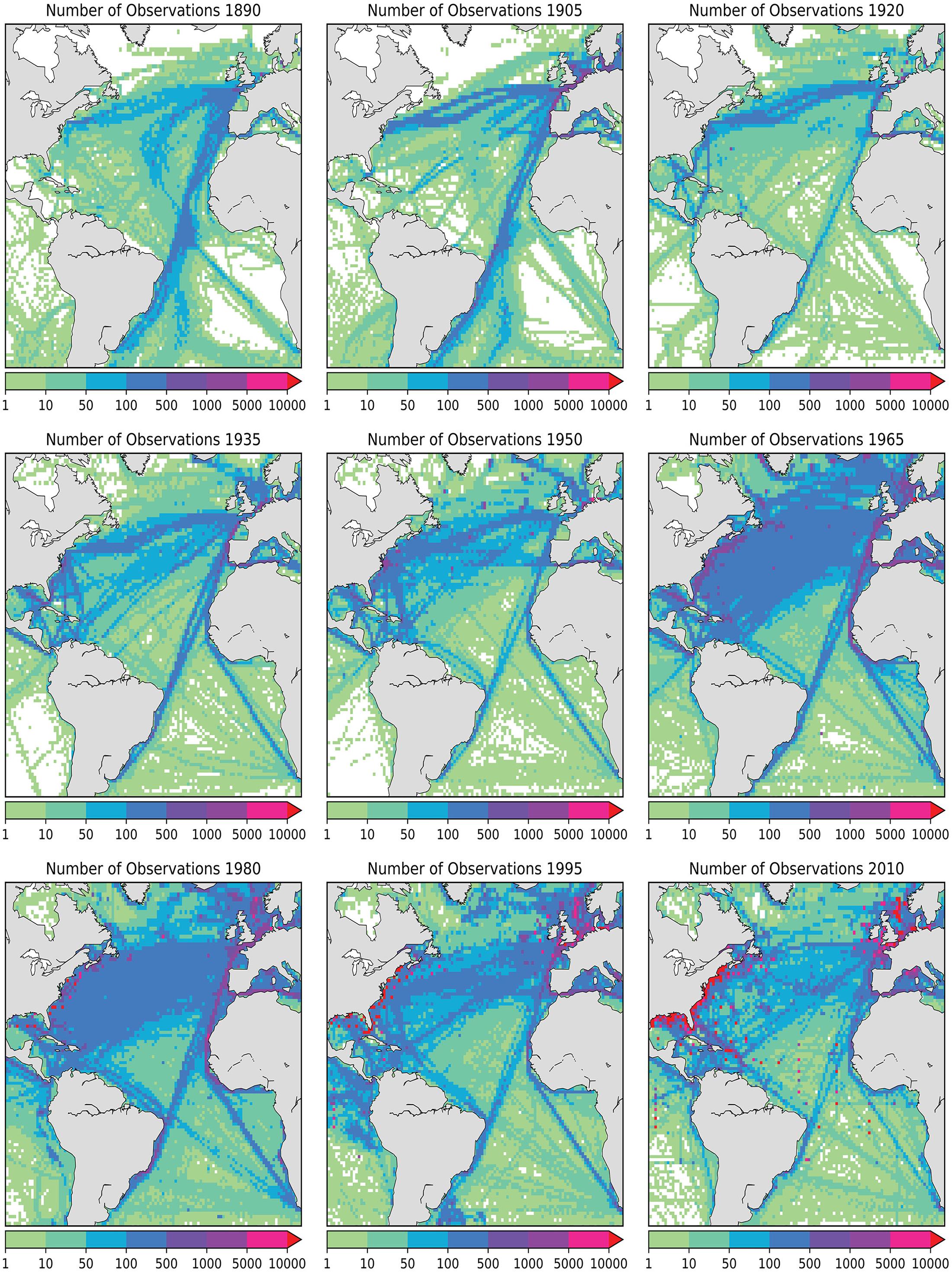
Figure 1. Annual number of ICOADS individual marine reports in one-degree latitude by longitude bins from 1890 to 2010 in 15-year increments. Observations per year are color coded according to the legend. Starting around 1980, moorings and fixed coastal stations appear as red squares indicating high data density.

ICOADS is composed of individual marine reports that include core parameters for time, location, and standard weather observations (e.g., wind, air and sea temperature, humidity, pressure, clouds, weather type, waves, and swell) along with metadata documenting instrument heights, data sources, and data quality. The contents of an individual ICOADS marine report are documented in the International Marine Meteorological Archive (IMMA) format (Woodruff, 2007; Smith et al., 2016) and the IMMA data may be obtained from NOAA National Centers for Environmental Information (NCEI). In our case, a database version of ICOADS, known as the ICOADS Value-Added Database (IVAD), is obtained from the National Center for Atmospheric Research’s Research Data Archive (Research Data Archive et al., 2016). IVAD contains the same content as the IMMA format ICOADS 3.0.0 but is organized in a MySQL relational database. In addition to selecting a subset focused on the last 125 years for the Atlantic basin, we further reduce the number of marine reports in our local ICOADS database by removing any records where the wind direction, wind speed, latitude, longitude, or year are null (missing).

There are several hundred source datasets that comprise ICOADS. These include archives of operational marine observations transmitted over the global telecommunications system (GTS), delayed-delivery datasets from ocean observing programs and national archives, and a host of other datasets created by digitizing historical logbooks and other marine weather records (Freeman et al., 2017). ICOADS tracks the source of observations using both a deck number (DCK) and a source identifier (SID). The DCK concept dates back to the first version of ICOADS (Slutz et al., 1985) where the source data are mostly read from “decks” of computer punch cards. Today, the DCK is used to identify a collection of marine reports (e.g., US Merchant Marine, UK Met Office Main Marine Data Bank), while the SID provides the source of the data and can comprise a single or mixture of decks. Data from a single SID are generally provided in a single original data format, prior to translation to the IMMA format. The quality and completeness of the marine reports in ICOADS are often related to the source of the observations (Freeman et al., 2017; see section “Data Quality Evaluation”).

The longest record of wind observations in ICOADS consists of wind direction and speed referenced to the fixed Earth, also known as a true wind (Smith et al., 1999). Early wind observations were made visually by observing the ship’s sails and later the sea state (e.g., Beaufort winds; Wheeler and Wilkinson, 2004). Mechanical, and more recently sonic, anemometers have been used for wind measurements since the early 1900s. Herein, we focus on developing indices of the zonal and meridional components of the wind, so both wind direction and speed are required (see section “Index Creation”). Wind directions in ICOADS have been measured using consistent methodology, including wind directions being reported as the direction from which the wind is blowing and a wind from the north being from 360° and from the east being 90°. There are variations in the precision of wind direction over the decades, with coarser 8- and 16-point compasses being used for visual observations evolving to wind observations precise to 1-degree increments with the use of anemometers (Figure 2). Inconsistencies in measurement practices for wind direction in ICOADS (i.e., resolution of wind direction) have very little impact on the wind component indices that we describe herein. The changes over time occur only for a fraction of data and have an impact on our wind component indices only when a vector component has a value of zero, which is largely addressed when we calculate the climatological probability density function (PDF) for our index (see section “Index Creation”). We envisioned more complicated wind-vector-based indices, using only portions of the probability distribution of vector components or applying weightings, where changing systematic errors in the wind speed (e.g., Thomas et al., 2005; Wheeler et al., 2010) could have resulted in spurious trends in the climate indices; however, we found that purely directional indices were sufficient to identify several modes of variability. Hence, we do not discuss wind speed calibration in this paper.

FIGURE 2

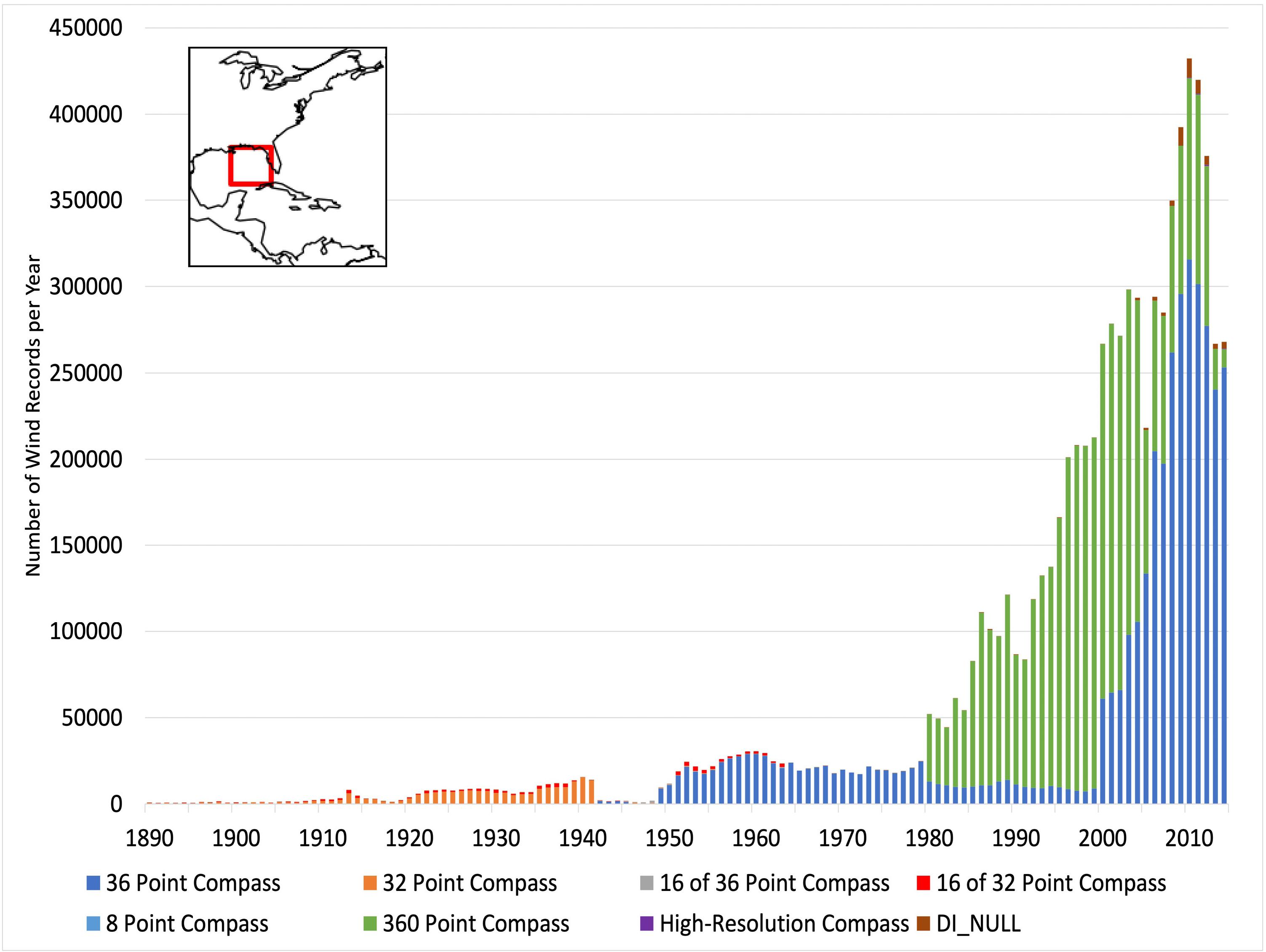
Figure 2. Annual count of ICOADS records for each wind direction indicator in the eastern Gulf of Mexico (see inset map) from 1890 to 2014.

Prior to the 1970s, almost all of the marine reports in ICOADS are ship observations. In recent decades, winds are observed by moored buoys, oil rigs, and other fixed and mobile ocean platforms. The type of observing platform is documented in ICOADS by a platform type (PT) indicator (Table 1). Taking the eastern Gulf of Mexico as an example (Figure 3), there is a notable increase in wind observations from moored buoys and Coastal-Marine Automated Network (CMAN) stations starting around 1980, and since 2000, observations from rigs, tide gauge stations, and other coastal stations are added to the platform mix. The authors note that the increase in winds from moorings and coastal stations is in stark contrast to the decline in ship wind observations, which started around 1980. As a result, in the open waters of the Atlantic a decrease in wind data density occurs after 1980 (Figure 1). The authors also note that the decline in observations for most PT after 2012 is simply the result of several delayed-mode datasets being incomplete for these later years when the data were ingested into ICOADS release 3 (Freeman, personal communication). The diverse mix of platform types and increased number of observations from buoys and CMAN stations can influence a wind-based index, resulting in variations that are not associated with wind variability (see section “Gulf of Mexico Index”). Another curiosity discovered when sorting wind observations by platform type is the fact that some PT associated with oceanographic profiling devices (e.g., bathythermographs, floats, CTDs, glider, and pinnipeds) have wind direction and speed observations within these marine reports. Since ocean profiling systems cannot measure winds, the authors initially planned to remove these wind observations. Through communication with the ICOADS development team, it was determined that these wind observations are not from the profiling instruments themselves, but instead are records of the wind observation on the platform (typically a ship) that is deploying the profiling device and that are taken near the time of device deployment. For that reason, these records are retained in the analysis.

TABLE 1

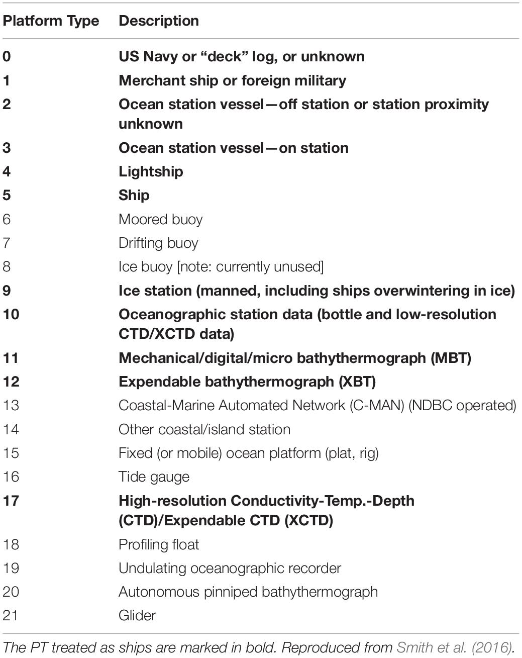
Table 1. Description of platform type (PT) indicators in ICOADS.

FIGURE 3

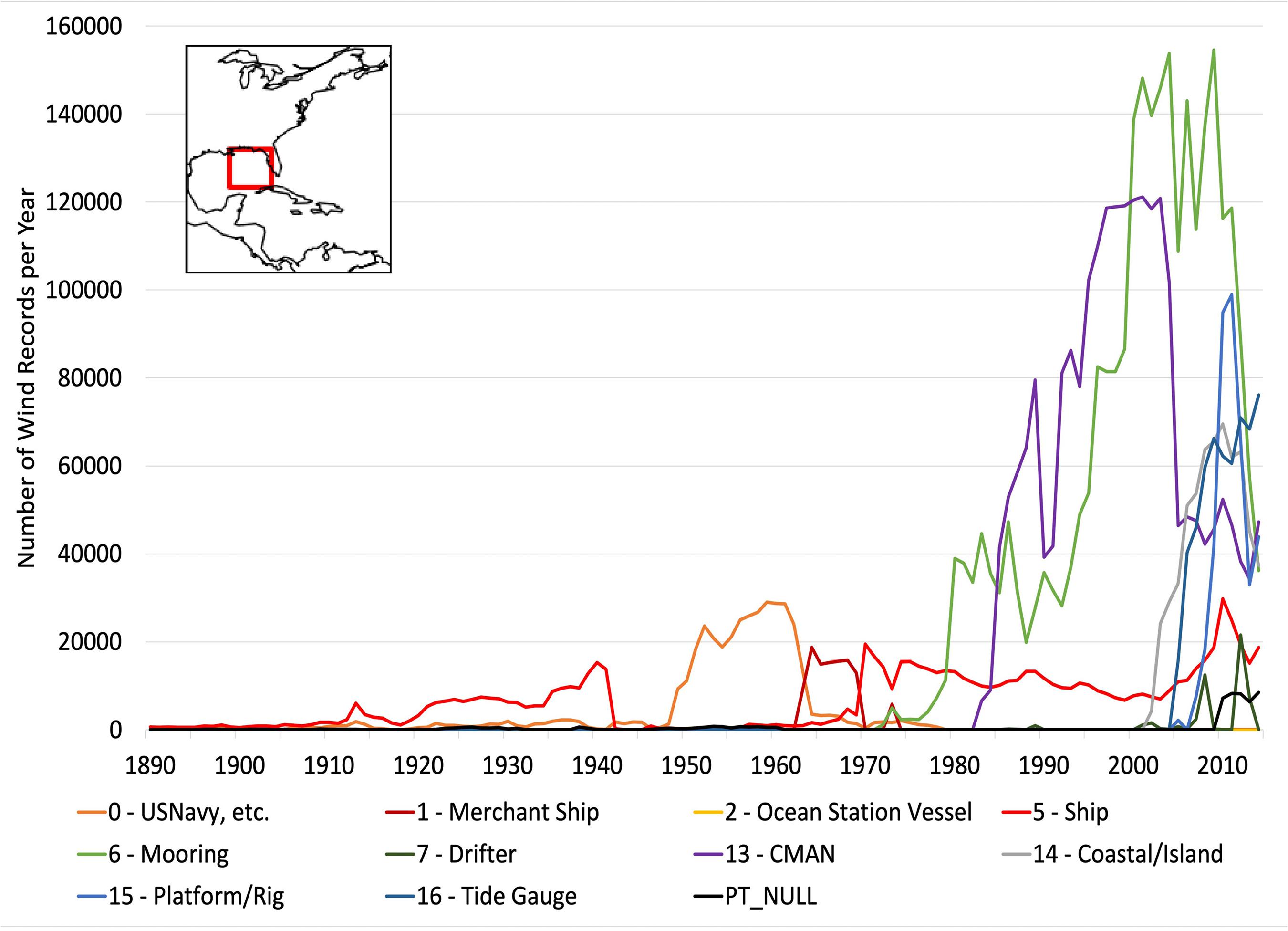
Figure 3. Annual count of ICOADS marine reports for each platform type in the eastern Gulf of Mexico (see inset map) from 1890 to 2014. Some types listed in Table 1 do not occur in this region, so are excluded from the graph.

Data Quality Evaluation

The diverse mix of wind observations in ICOADS also results in these observations having varying quality, which is assessed prior to construction of wind component indices. First, we examine the distribution of wind speed for each of the decks to determine if the distribution fits a reasonable expectation for wind speed over the ocean. A reasonable wind speed distribution is exemplified by the GTS observations received by the National Center for Environmental Prediction in the Binary Universal Form for the Representation of meteorological data (deck 793; Figure 4A), which contains over 21 million reports collected across the global oceans from 1998 to 2014. The distribution exhibits the expected peak occurrences around 6 ms^–1 with lower frequencies at lower speeds and a tail skewed toward higher wind speeds. The distribution of deck 793 is similar to those from other large global decks [e.g., International Maritime Meteorological (deck 926); NCEI GTS: Ship Data (deck 992), not shown]. Two decks, US Navy METAR hourly (708) and the World Ocean Database/Atlas (780), exhibit unrepresentative distributions (Figures 4B,C). Deck 708, with records from 2001 to 2012, consists of only low winds (<5 ms^–1) and deck 780, from 1890 to 2014, has an unrealistic peak at 0–0.9 ms^–1. To avoid bias in the wind indices, decks 708 and 780 are completely removed from this analysis. In addition, we remove deck 874 (SEAS project data) as this deck has been previously documented to be incorrectly translated from the SEAS format into IMMA (Freeman et al., 2017).

FIGURE 4

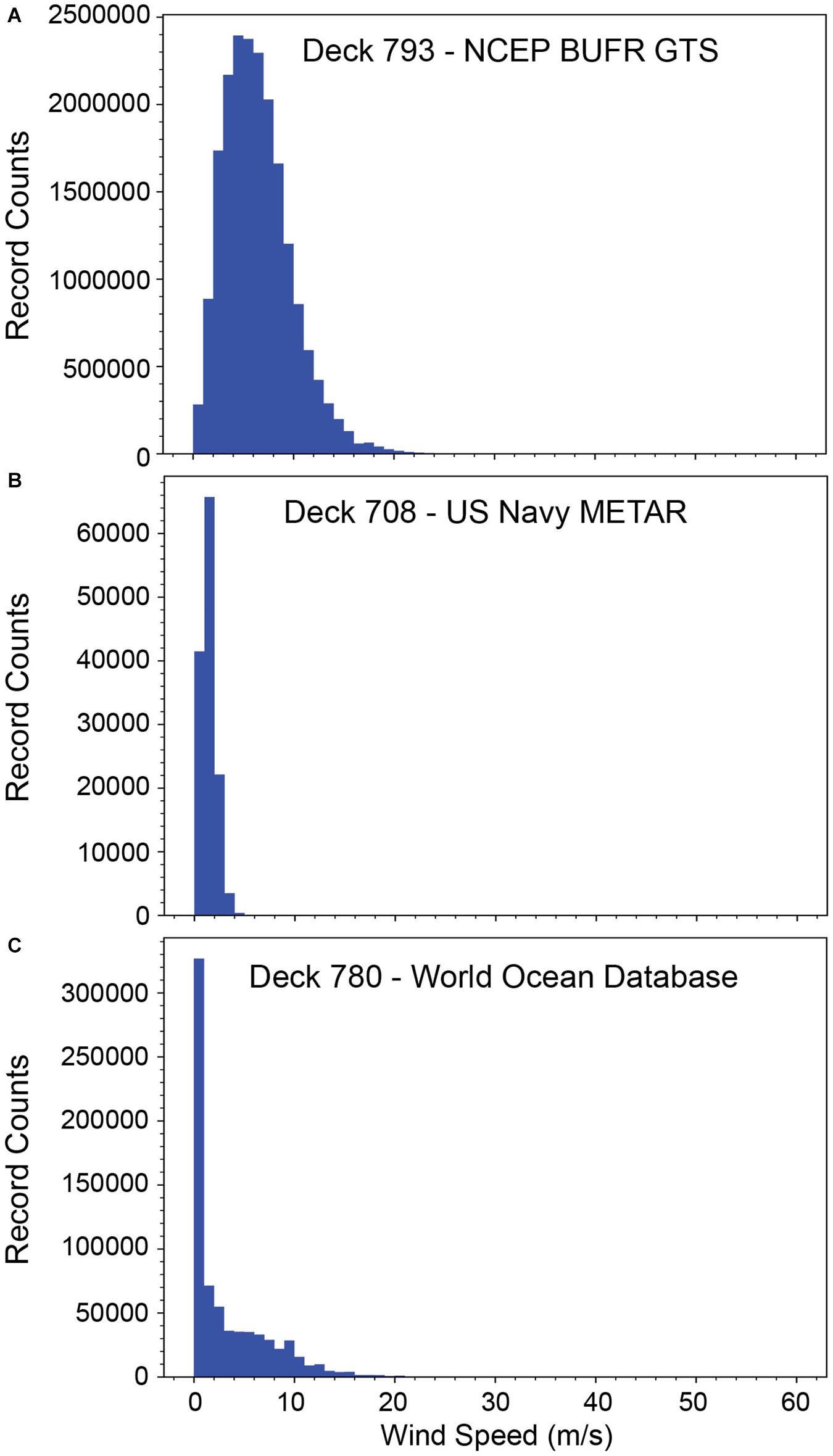
Figure 4. Comparison of wind distributions from ICOADS decks (A, top) 793, (B, middle) 708, and (C, bottom) 780.

Limited quality control of individual wind reports in ICOADS has been conducted. Slutz et al. (1985) provided flow charts of ICOADS wind tests that were based on procedures developed by the National Climatic Data Center (NCDC). These NCDC flags were stored in the WNC flag in IMMA and include internal consistency checks between the wind speed, present weather conditions, and visibility; internal consistency checks between wind speed/direction and wave height/period; ensuring wind direction is within the valid range of 1–362 (note: in ICOADS a direction = 361 represents a calm wind; direction = 362 represents a variable wind); and a check to ensure that 0 ≤ wind speed ≤ 102.9 ms^–1. Failures of these tests resulted in WNC flags for legality and internal consistency, and records with these WNC flags are removed prior to index creation. The legality and internal consistency flags are accepted primarily because the tests outlined in Slutz et al. (1985) seem reasonable and retesting is beyond the scope of our research. We also verify that the NCDC quality checks that ensure the calm and variable wind directions are consistent with their respective wind speeds.

The NCDC quality control also flagged wind speeds as erroneous if they were outside ± 5.8 standard deviations from the mean, based on outdated 5° latitude by 5° longitude box long-term monthly means derived from pre-ICOADS data from NCDC (Slutz et al., 1985, NOAA, 2016). A second wind “trimming” flag was applied to the wind components calculated by the ICOADS team as part of the creation of binned monthly products (Slutz et al., 1985). Examination of high wind speed observations in ICOADS reveals an inconsistent application of the WNC flags. The number of occurrences of wind speeds > 50 ms^–1 for each deck is calculated and over 70% of these high wind measurements are from three decks: 892 (39.6%), 732 (21.1%), and 992 (11.0%). For both the WNC (Figure 5A) and the ICOADS trimming flags (Figure 5B), numerous wind speeds greater than 50 ms^–1 are identified as “good,” regardless of which deck or year of data is examined. The existence of many unflagged high wind speeds results in a lack of confidence in the WNC sigma and ICOADS trimming flags, and neither is applied in this analysis. After further consideration of the expected wind distributions (e.g., Figure 4A), the authors exclude any wind observations (speed and direction) when the wind speed was greater than 40 ms^–1.

FIGURE 5

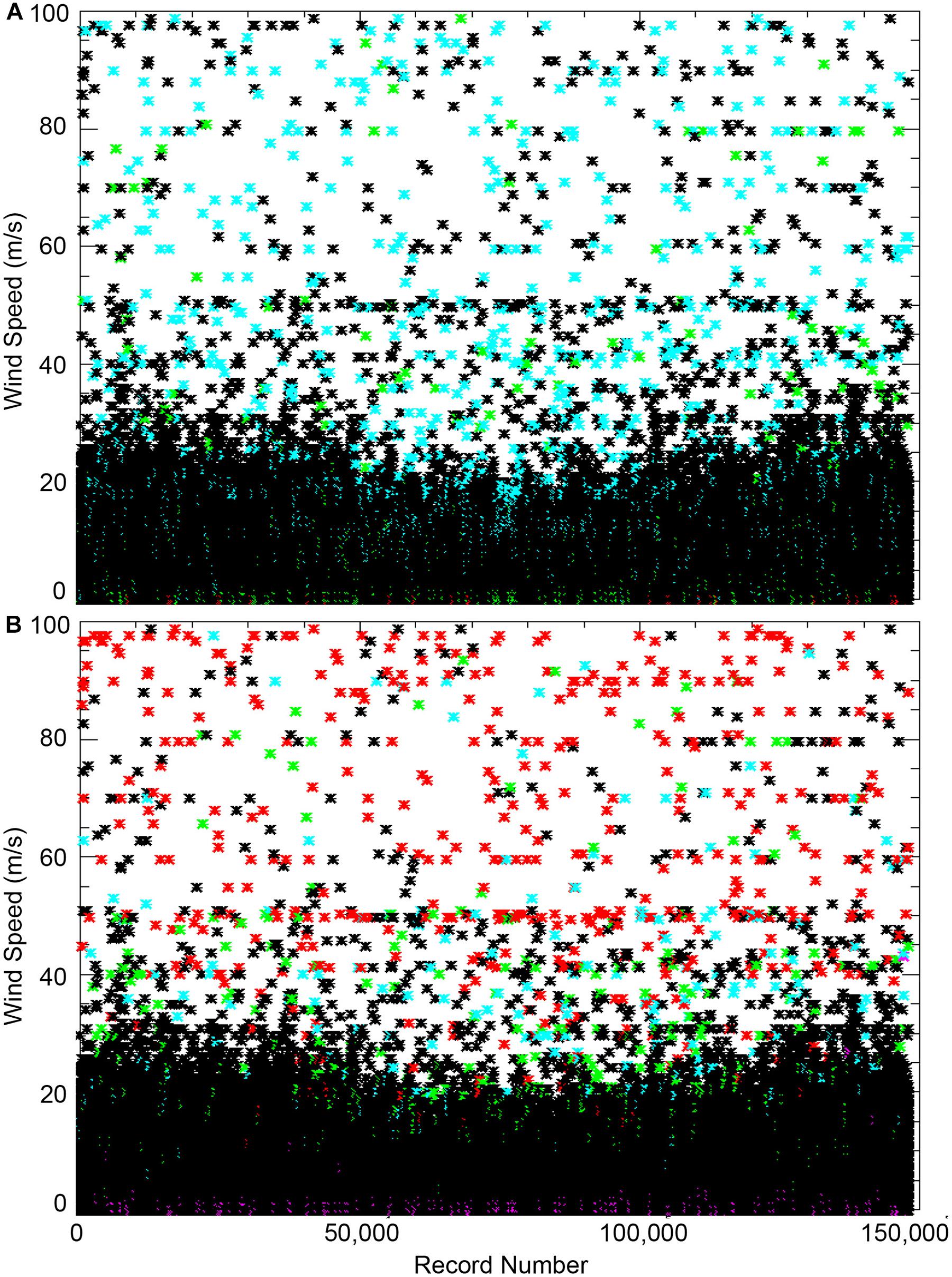
Figure 5. Wind speeds from 1985 for deck 892 color coded by (A, top) WNC flag = good (black), correctable (green), suspect (blue), and erroneous (red) and for (B, bottom) trimming flags within 2.8 sigma (black), within 3.5 sigma (green), within 4.5 sigma (blue), and outside 4.5 sigma (red). The plot displays winds for approximately 150,000 records available for this deck and year.

Additional tests are conducted to identify incorrect dates, platform positions over land, and suspect platform identification. At times marine reports in ICOADS do not include a value for the day of the month. Although we flag these null days, these records are still included in the annual or seasonal indices. The NCDC quality control from ICOADS also includes a ZNC flag, which is used to identify incorrect times or positions of platforms over land. If a report falls over a land box as indicated by a land mask defined in Slutz et al. (1985), it is flagged ZNC = 7 (erroneous via legality). Note that ZNC = 7 can also be set by NCDC-QC for other reasons, such as missing hour or day. Additionally, if a report falls over a 2° land box as indicated by a NCDC landlocked file (see supplement G, section 2 in Slutz et al., 1985), a separate ICOADS landlocked flag is set: LZ = 1 (report over land). During creation of the final IMMA for release 3.0, reports with LZ = 1 are not output, and we confirm that there are no records with LZ = 1 in the available ICOADS records; however, 649,412 records have ZNC = 7. Of these, 468,159 have null values for time, representing ∼72% of values where ZNC = 7. The other 28% of values are presumed to be flagged because of their proximity to land, rather than any issues with time, as these records have existing and valid (but not necessarily correct) time values. Since the NCDC quality check for position over land uses a coarse land mask, we conduct an additional position check comparing the individual records’ latitude and longitude against the ETOPO1 arc-minute topographic map (Amante and Eakins, 2009). The test follows the approach used in Smith et al. (2018), and we remove any records where the topographic elevation is greater than zero meters. Finally, we remove any records with a platform identifier (e.g., ship call sign or buoy number) that contained non-alphanumeric values. These identifiers may be correctable, but, again, this is beyond the scope of the project.

Again taking the eastern Gulf of Mexico as an example, the result of all the QC tests is the removal of 7.2% of the 8,059,556 ICOADS records with available wind observations from 1890 to 2014. Of the 583,908 records removed, the majority (80%) are for positions identified as over land. Approximately 1% of the records are removed because they failed the NCDC legality or internal consistency checks, 0.4% had suspect platform identifiers, and 0.15% had wind speeds greater than 40 ms^–1. Similar QC results are expected for other high data density regions prior to any index creation.

Index Methodology

Index Creation

A methodology that provides the ability to create an extensive suite of climate indices using a probabilistic approach is developed. The indices are created over regions that typically manifest atmospheric circulation patterns indicative of various climate phenomena. A region over which to create an index is selected based upon: (1) climatological interest and (2) a consistently high observation density over multiple decades (Figure 1). Geographic coordinates are selected to create a rectangle region around the area of interest. A tool to create a more refined polygon around the area of interest has been tested, but no advantage over the use of a rectangle shape is exhibited for our test cases (see section “Gulf of Mexico Index”). An added benefit of this methodology is the capability to create an index using different variables. The index method has been tested for wind component, wind speed, wind direction, and surface pressure variables. To demonstrate the index method, a test case using wind components will be referenced for the remainder of this section.

Wind component indices to be used for illustrating climate phenomena in the Atlantic subset region are developed using quality-controlled wind variables from ICOADS R3.0.0. The wind component indices are developed for horizontal wind vector components only. Although wind vector component variables do not exist in the ICOADS database, the available wind speed and wind direction variables are used to derive the horizontal wind vector components for the PDF calculations. The wind vector components are derived by:

$u=Ucos({270}^{°}-\theta )(1)$

$v=Usin({270}^{°}-\theta )(2)$

where u is the zonal wind component, v is the meridional wind component, U is the wind speed, and θ is the wind direction. When calculating the horizontal wind components, we must address calm and variable winds. Recall that ICOADS defines calm wind to have a wind direction of 361° and variable wind to have a wind direction of 362°. The horizontal wind components are set to 0 ms^–1 under the circumstance of a wind vector with a wind magnitude of 0 ms^–1 and wind direction of 361°. If the wind magnitude exceeds 0 ms^–1 when the wind direction is 361°, the horizontal wind component calculations are excluded for this data point as the wind magnitude does not correspond to a calm wind. For any case in which the wind direction is equal to 362°, the horizontal wind component calculations are omitted. This procedure can be thought of as excluding observations for which vector components are ill defined, or arguably as ignoring conditions where winds are clearly driven by small spatial/temporal scale processes. If such conditions are important to the phenomenology being investigated, then this part of our procedure should be reconsidered.

PDFs are used to develop the wind component indices. For a wind component, PDFs are calculated for a region and time period based upon the aforementioned criteria to determine the probability of occurrence within a specific range of wind component values. These PDFs are calculated over an accumulation interval: monthly, seasonally, or annually. The advantages of using PDFs include independence of sample size and being relatively insensitive to random error.

Wind component indices are created to characterize changes in the probability of wind vector components above or below a threshold (x_th), where x is a vector wind component. For this study, a threshold of zero was used, meaning we are examining the varying probability of a positive or negative horizontal wind component within a study region. While shifts in probability could be examined directly as demonstrated by Wheeler et al. (2010), it seems more useful to examine changes relative to a base state defined by calculating a climatological PDF (Figure 6) for the region and part of the year being considered. As mentioned before, we considered developing indices that used only portions of the PDF; however, we found that was not necessary. To calculate the climatological PDF, we use the following method of converting a histogram into a PDF:

FIGURE 6

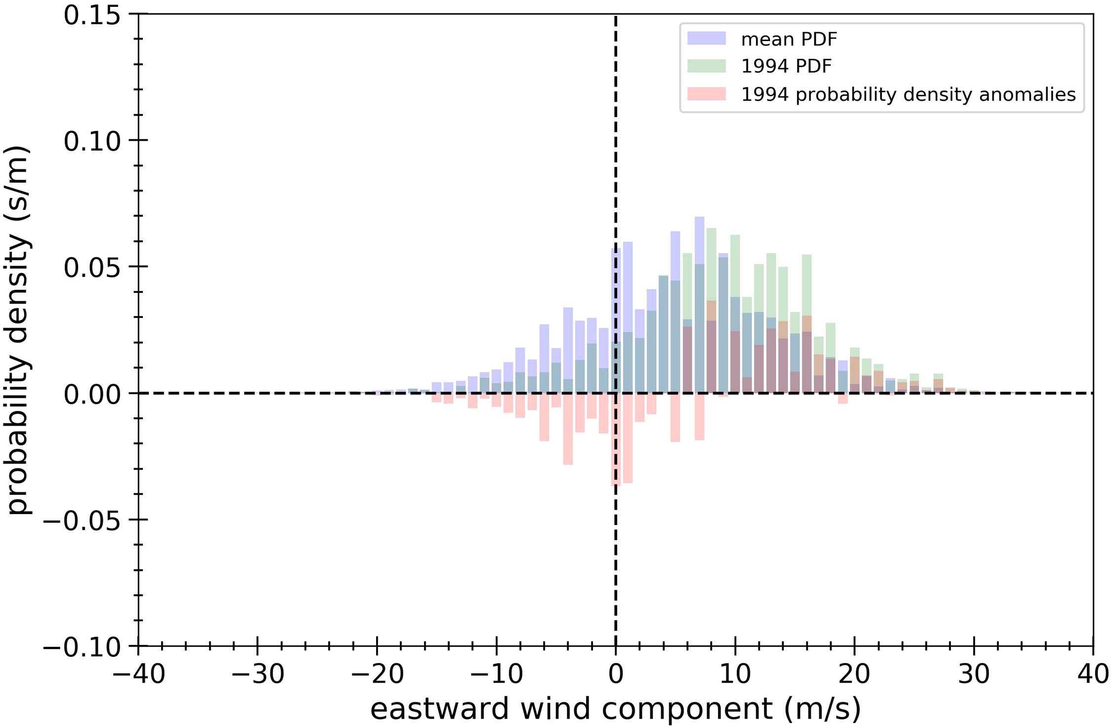
Figure 6. Zonal wind component probability density function (PDF) for 1994 DJF (green), climatological mean probability density function for 1890–2014 DJF (blue), and probability density anomalies for 1994 (red) for the region: 45° to 55°N and 15° to 25°W.

$PD{F}_i=\frac{n_i}{\sum (n_i\mathrm{\Delta }{x}_i)}(3)$

where n_i is the count value for the observed wind component values that fall in the i^th range of vector component values (x_i ≤ x < x_i+1) and Δx_i = x_{i + 1}−x_i is the width of this i^th range. Using Eq. 3, an individual PDF is calculated for each accumulation interval within each year of the climatological period. For all index calculations discussed in this paper, the Δx has been held constant at 1.0 ms⁻¹. For all PDF calculations, the counts for 0.0 ms⁻¹ are split equally between the [–1, 0) and [0, 1) ms⁻¹ bins. This is done to eliminate a bias toward positive horizontal wind component probability densities, as all counts for 0.0 ms⁻¹ would fall into the [0, 1) bin otherwise. The climatological PDF is obtained by calculating the mean probability density of each bin over the selected climatological period (e.g., 1890 to 2014 winters defined as December-January-February in Figure 6).

For each accumulation interval (t) over the climatological period, probability density anomalies are calculated for each bin (i):

$PDF{A}_{i,t}=PD{F}_{i,t}-PD{F}_{mean,i}(4)$

where PDFA_i,t is the anomalous probability densities for wind bin i and time t, PDF_i,t is the probability density function of an individual accumulation interval, and PDF_mean,i is the time mean probability density function calculated for the climatological period. The anomalous probability densities reveal how the occurrences of the horizontal wind components over the accumulation interval deviate from the climatological PDF (Figure 6). We find these shifts in PDFs to be insightful for describing how the winds differ from the climatology, which is useful when selecting x_th. All probability density anomaly (PDFA) values associated with wind component values greater than the threshold are added up to a total value, and the probability density anomaly values associated with values lower than the threshold are added up to a total value. The non-standardized index value (I_NS) is calculated by finding the difference of two sums of the total probability density anomaly values for the wind component:

$I_{N{S}_t}=\sum _{i}PDF{A}_{i,t}(x|x>x_{th})-\sum _{i}PDF{A}_{i,t}(x|x<x_{th})(5)$

A positive (negative) index value indicates more occurrences of wind component values greater than (less than) the threshold. The non-standardized index value is standardized because not only is the raw index a relatively small value, but the standardization emphasizes the departure from the mean relative to the variability of the index:

$I_t=\frac{(I_{N{S}_t}-\overline{I_{NS}})}{S_{I_{NS}}}(6)$

where I_t is the index value for an individual accumulation interval at time t, $\overline{I_{NS}}$ is the mean index value over the climatological period, and S_{I_NS} is the standard deviation of the non-standardized index values over the climatological period. By taking this approach, units on the index value are eliminated, and the scale of the departure is more easily understood as a number of standard deviations rather than a shift in probability. This standardization process effectively removes the need to consider the climatological PDF because the use of that PDF shifts the non-standardized index by a constant, which is accounted for by subtracting the mean index. If more non-uniform weighting was applied, or if only portions of the PDF were used, then the climatological PDF remains important.

There are several differences from the directional indices created by Wheeler et al. (2010). A minor difference is that we consider all vectors within 90° of a cardinal direction rather than within 45° of a cardinal direction. This is likely a very minor difference. A more important difference is that we consider increases in eastward winds simultaneous with decreases in westward winds, which emphasizes shifts in a PDF more than increases in a specific cardinal direction, which could also be due to changes in curvature of flow. The importance of this difference in approach depends on the type of circulation that is being examined. Another difference in these approaches to determining wind indices is the scaling that we have done to show the magnitude of anomalies in terms of standard deviations. The above differences are likely to be minor for most applications. Another difference is that Wheeler et al.’s indices are based on changes in frequency of daily averaged winds, whereas we examine a distribution determined from spans of space and time. When winds are well sampled in time, there will be only small differences in results. However, our experience in creating the monthly Florida State University winds products (Bourassa et al., 2005) has shown that areas with poor temporal sampling can have winds that are not representative of the monthly averaged winds, whereas sampling over a larger span of space and time usually results in a reasonable monthly average. This experience shows the beneficial impact of using larger sample sizes in reducing the noise in the indices. The next section on the uncertainty in our index shows how the number of observations influences uncertainty.

Index Uncertainty

The uncertainty in the standardized index σ_t for each time ‘t’ is determined by treating the wind vector component as being binary (that is, either below the threshold or greater than the threshold, after values that are equal to the threshold are split evenly between these two categories). The probability (p_t) of an event being greater than or equal to the threshold is equal to the number of observations in this category divided by the total number of acceptable observations. The probability (n_t) of a vector component being less than the threshold is equal to 1 – p_t. Based on the Wald method (Laplace, 1812) for determining confidence limits, the uncertainty (σ) for one term in each of the differences in (5), expressed as one standard deviation, is equal to:

$\mathrm{\sigma }=\sqrt{p(1-p)/n}(7)$

For a wind component index, we treat the fraction of the PDF’s values for positive vector components as totally dependent on the fraction of negative values, which implies that the uncertainty for the difference of these terms is double the value in (7). The uncertainty in the difference of fractions for the climatological PDF has a similar form, but uses the climatological values for p and n. If the uncertainties in the climatological term are treated as independent from the annual or seasonal term (which will very slightly underestimate the uncertainty), then these uncertainties can be added in a root mean square sense:

${\mathrm{\sigma }}_t=2{[\frac{p_{A_t}\left(1-p_{A_t}\right)}{n_{A_t}}+\frac{p_C\left(1-p_C\right)}{n_C}]}^{0.5}/S{}_{I_{NS}}(8)$

where the subscript ‘A’ indicates the accumulation interval for the PDF, the subscript ‘C’ indicates the value for the climatological PDF, and S_{I_NS} is the standard deviation of the series of non-standardized index values. The index uncertainty represents one standard deviation of an error distribution that is assumed to be a Gaussian distribution. This uncertainty is greatly dominated by the uncertainty in the annual (or seasonal) PDF, which is largely influenced by the number of observations.

There are several approaches to determining if an index of climate or weather variability is useful. One measure of usefulness of a climate index is the ability to find a signal that stands out well above the noise. On annual and seasonal scales this index has a noise that is much smaller than the signal through the time period that is examined, as is demonstrated in the next section. Another validation technique is to compare the new index to an accepted index. Similar to Wheeler et al. (2010) a directional index for the NAO is compared to other NAO indices, and found to be reasonably similar (section “Validating the Method”). Lastly, in section “Results: Gulf of Mexico Case Study” we demonstrate that a directional index for the Gulf of Mexico can be used to usefully explain decadal and multi-decadal rainfall variability.

Validating the Method

A wind component index developed for the north Atlantic region validates the use and demonstrates the efficacy of the methodology discussed. Specifically, a winter (December-January-February; DJF) zonal wind component index for the region 45° to 55°N and 15° to 25°W (Figure 7 inset) over 1890 to 2014 is constructed to illustrate the phases of the NAO. This geographical box falls along a defining region of the NAO: the midlatitudes over the Atlantic Ocean, where the upper branch of the Azores High meets the lower branch of the Icelandic Low. The dynamic interaction between these two regions generates pronounced westerly flow. During a positive NAO phase, the Azores High and Icelandic Low are anomalously strong, increasing the pressure gradient between the two systems. Consequently, strong westerly winds result in the midlatitude region over the north Atlantic. Anomalously weak westerly or easterly winds are present in the region during a negative NAO phase as the gradient between the Azores High and Icelandic Low is anomalously weak. To capture the dynamic behavior of the NAO, a zonal wind component index (hereafter referred to as zonal NAO index) is developed to monitor the zonal wind characteristics within this midlatitude region. Knowing the wind behavior during NAO phases, we can expect positive (negative) zonal NAO index values to suggest the occurrence of a positive (negative) NAO phase, similar to the findings of Wheeler et al. (2010). The zonal NAO index suggests a primarily positive NAO phase for the 1904–1927 winter seasons. More variability between positive and negative NAO phases is seen in winter seasons post 1950, with a strong negative NAO phase suggested for 1964 and 2010 winter seasons and a strong positive NAO phase suggested for 1960, 1993, and 1994 winter seasons (Figure 7).

FIGURE 7

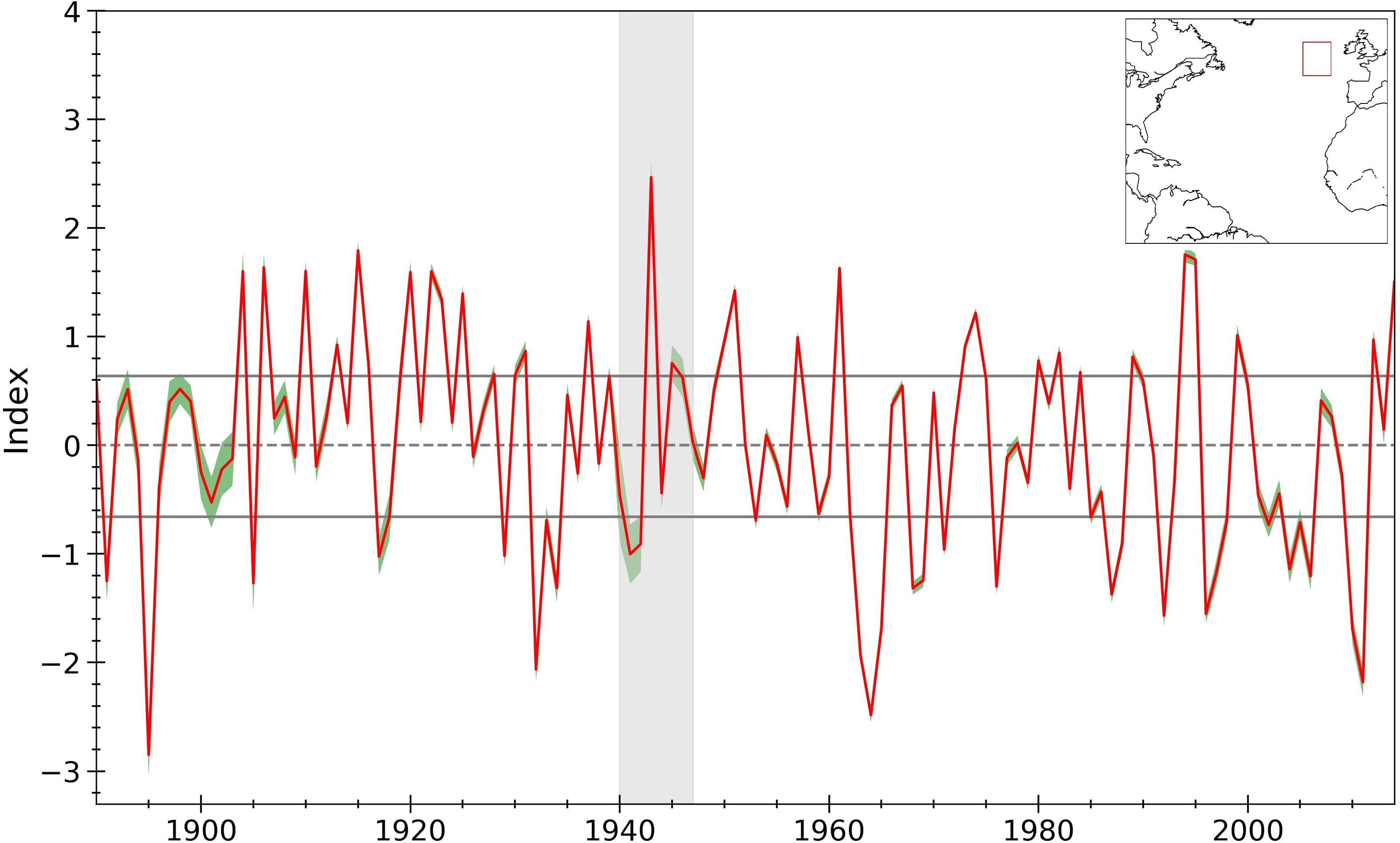
Figure 7. 1890–2014 time series of the standardized zonal wind component index for the region: 45° to 55°N and 15° to 25°W (see inset map). Uncertainty in the index is shaded in green. The gray solid horizontal lines represent the 25th and 75th percentiles and the gray dotted lined represents the mean standardized index. The gray shaded area denotes WWII years where ship data became sparse.

To validate this new probabilistic method, the zonal NAO index is compared to two operational indices that monitor the NAO: a station-based NAO index and the EOF-based NAO index (Figure 8A). The station-based NAO index was developed by calculating sea level pressure differences between Lisbon, Portugal, and Reykjavik, Iceland, while the EOF-based index was derived from the leading EOF of SLP over the Atlantic (20°-80°N, 90°W-40°E; Hurrell et al., 2003). The record for the station-based NAO index extends from 1864 to present day, whereas the EOF-based NAO index extends only from 1899 to present day. The data for both station-based and EOF-based indices are obtained from NCAR Climate Analysis Section (2003). The zonal wind NAO index highly correlates (r = 0.6597) with the station-based index and shows a moderate correlation (r = 0.39629) with the EOF-based index (Figure 8B). A higher correlation with the station-based index is expected as this operational index and the zonal wind index are created using observational data. Additionally, both the zonal wind index and station-based indices detect small-scale variabilities in the pressure, and consequently wind, fields that the EOF-based index does not reflect. This is because the EOF method aims to find the largest scale repeatable variability over a broad spatial domain, causing the small-scale variability to become lost. We state that these indices highly and moderately correlate with one another because the zonal NAO index is shown to capture a NAO-like signal using a different variable and different spatial scales. A perfect fit is not desired between the indices; otherwise, the new index methodology proposed would be providing neither a different perspective nor new information on the climate phenomena. A similar test and outcome can be found in Wheeler et al. (2010). To analyze long-term variations, a 7-year moving average (see section “Correlation Between Gulf of Mexico Component Indices and Precipitation”) is applied to the zonal NAO index and the two operational NAO indices. With a 7-year moving average, the zonal NAO index exhibits the same multidecadal patterns that the two operational NAO indices detect (Figure 8C). With certainty in the probabilistic method for creating climatic indices by testing a popular climate phenomenon, this method will be further demonstrated for an index in the eastern Gulf of Mexico.

FIGURE 8

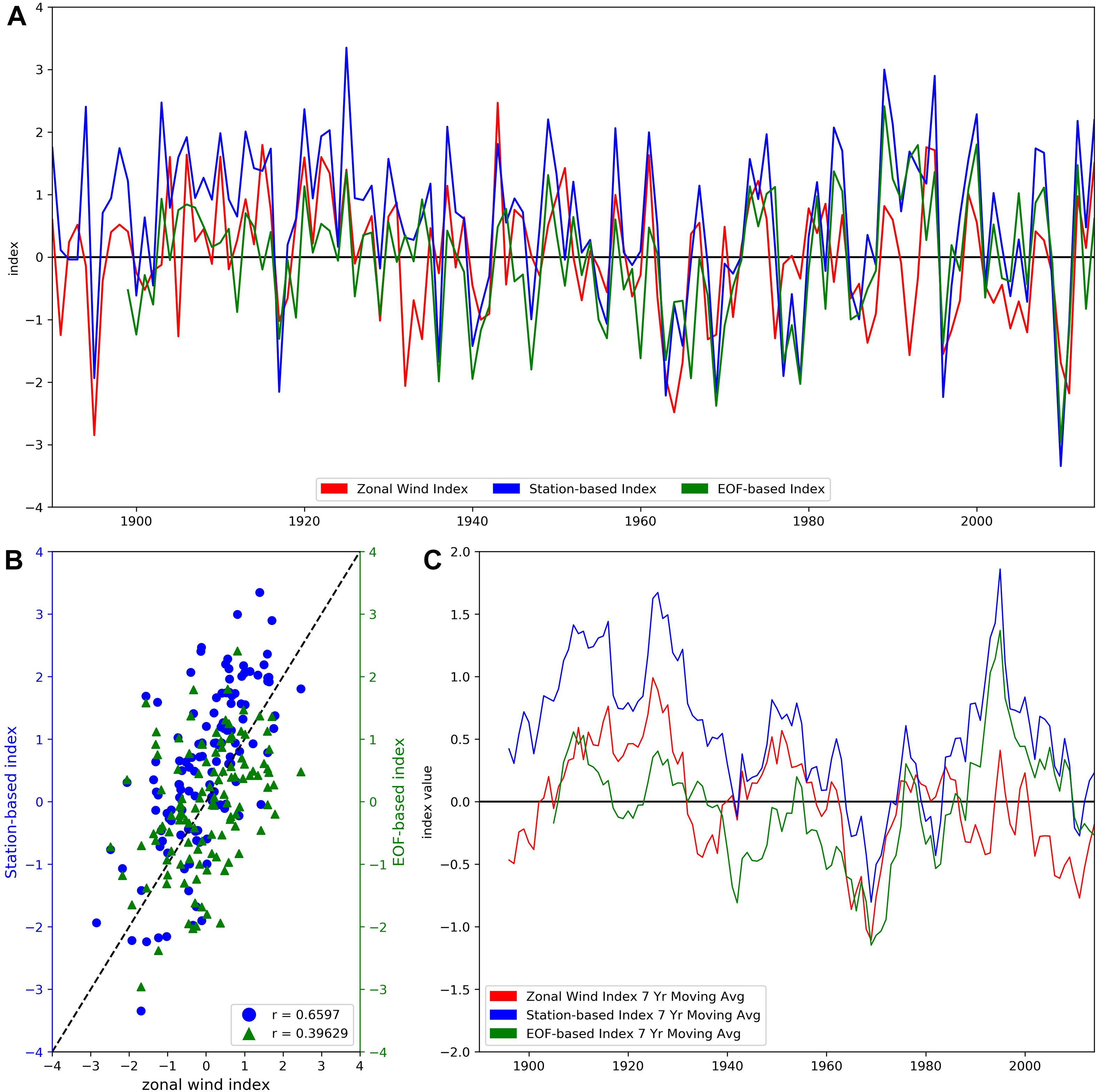
Figure 8. (A, top) 1890–2014 time series of the standardized zonal wind component index (red) for the region 45° to 55°N and 15° to 25°W, 1890–2014 station-based NAO index (blue), and a 1899–2014 EOF-based NAO index (green). (B, bottom left) Scatterplot of zonal wind index vs. station-based index (blue circles, r = 0.6597) and zonal wind index vs. EOF-based index (green triangles, r = 0.39629). A 1:1 line (black dashed line) is used to aid in visual correlation. (C, bottom right) 1890–2014 time series of 7-year simple moving averages, i.e., rolling mean, of the zonal wind index (red), station-based index (blue), and the EOF-based index (green).

Results: Gulf of Mexico Case Study

Gulf of Mexico Index

Annual zonal and meridional indices are created spanning 1910–2014 (data density prior to 1910 is too sparse) for the eastern Gulf of Mexico (23°-30°N and 82°-90°W; Figure 9A inset). This region was selected to encompass the primary ship route from the Florida Straits to the mouth of the Mississippi River and includes the highest data densities in the eastern Gulf of Mexico (Figure 1). The zonal index, constructed using all available platform types and only observations that pass all of the quality control outlined in section “Data Quality Evaluation” (Figure 9A), has a clear interannual variability with values centered on -0.5 from 1910 to approximately 1980. Thereafter, the index shows a striking increasing trend toward positive values, albeit with substantial year-to-year variability. The trend is toward more occurrences of eastward winds in the region after 1980.

FIGURE 9

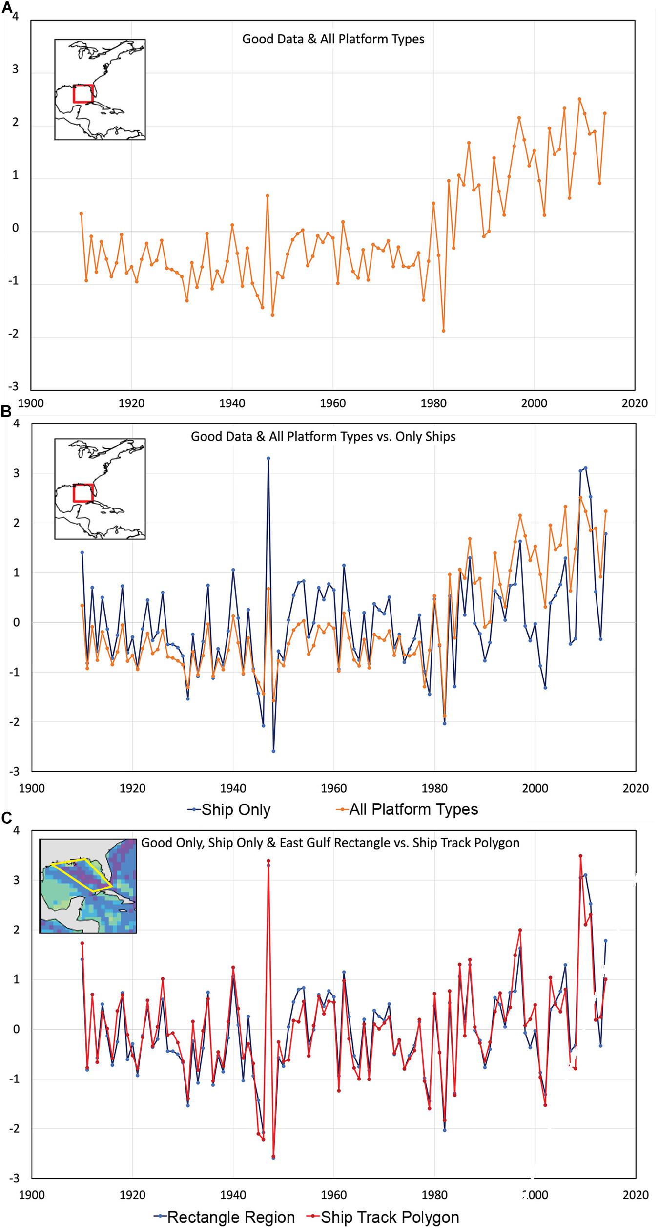
Figure 9. Eastern Gulf of Mexico zonal wind index (A, top) created using all available platform types and a rectangular region (see inset map), (B, middle) comparing all platform types (orange) to using only ship observations (blue) for the rectangular region (see inset map), and (C, bottom) comparing the ship-only indices created using a rectangular region (blue) to a polygon following the high-density ship track (red). The inset map for the polygon shows the ICOADS data density for 1970 when ship traffic was at its maximum using the color scale from Figure 1.

Although the post-1980 trend in the zonal index is striking, heterogeneity of ICOADS observing platforms requires careful consideration of which wind observations are used when creating wind component indices. The trend toward an increase in occurrences of eastward winds (Figure 9A) starts near 1980, which corresponds to the increase in wind observations from moored buoys and CMAN stations (Figure 3). To assess the impact of these modern observing platforms, the authors recomputed the index using only ship observations. Ship observations are defined as having PT = 0–5, 9–12, and 17 (Table 1). The result was a noticeable difference in both the zonal (Figure 9B) and meridional (not shown) indices after 1980, but an upward trend toward more eastward winds is still apparent when only ship observations are used. Differences in the magnitude of the zonal index also exist prior to 1980, for which time variations center more on an index value of zero, but the overall trend is relatively flat using only ship observations. We attribute the difference when using non-ship wind observations to the fact that CMAN and other coastal stations measure winds in a regime (e.g., sea/land breeze circulations, locations more prone to turning associated with frictional convergence and divergence) that is very different from the open ocean and these stations tend to report winds at sub-hourly time intervals, thus overwhelming the ship observations, which are typically made every 3 to 6 h.

A further consideration is whether or not the region of the ocean selected influences the resulting index. To examine this for the eastern Gulf of Mexico, we selected a polygon that bounded the primary ship track spanning from the northern coast of Cuba northwestward to the northern Gulf Coast (Figure 9C). The resulting annual zonal wind index, calculated using only ship observations that passed all quality-control tests, is very similar to the index calculated using the rectangular region shown previously (Figure 9C). The conclusion is that as long as the region selected encompasses the high-density ship tracks, the actual shape of the region does not matter. This is reasonable since we are using a PDF approach and the bulk of the data in the PDF come from the regions with the highest sampling density.

Correlation Between Gulf of Mexico Component Indices and Precipitation

The ability to link a wind climate index to variability in a non-wind observation is a practical indicator that the index is effective. These wind component indices provide the opportunity to explore potential spatiotemporal relationships with precipitation in the southeastern and Gulf Coast states, including the use of the onshore/offshore wind component index as a metric that may benefit future prediction of seasonal or annual precipitation anomalies to support the agricultural sector. This analysis examines the variability in rainfall on a seasonal basis and applies multiple linear regression analysis to relate the zonal and meridional components for the eastern Gulf of Mexico (23°-30°N and 82°-90°W) to the seasonal precipitation in the Gulf Coast states. Similar to the annual index for this region (Figure 9B), we create seasonal wind component indices using only ship observations and those data that passed all the quality-control tests (e.g., good data) for the precipitation analysis.

The precipitation data are from the Global Precipitation Climatology Centre (GPCC) global land-surface precipitation data products (Becker et al., 2013). The analysis product is based solely on rain gauge stations, near real-time and non-real-time, in the GPCC database that supply data for each month. The GPCC Full Data Reanalysis Product Version 7 covers the period from 1901 to 2013 on a 2.5° latitude and longitude grid, with each grid cell containing the areal average precipitation and number of gauges for the given month. The global number of stations per month contributing rain data varies from less than 10,000 to more than 48,000.

Due to the relatively coarse grid spacing of the GPCC precipitation dataset, individual grid cells along and adjacent to the immediate Gulf of Mexico coastline are selected. These cells span northeastern Mexico, the southern regions of Texas, Louisiana, Mississippi, Alabama, Georgia, South Carolina, and the Florida peninsula (Figure 10). These cells are selected because the Gulf of Mexico is the primary moisture source for precipitation along the Gulf Coast, and we hypothesize that variations in winds in the northeast Gulf of Mexico may be indicative of changes in moisture available for precipitation over the continent. Since the precipitation dataset is based on rain gauge observations, there are no grid points over the open waters of the Gulf of Mexico. Some of the cells are centered over the Gulf, but these cells represent the limited coastal or island gauges near the edges of the grid cell. Finally, the grid cells centered on 28.75°N, 86.25°W, 26.25°N, 83.75°W, and 23.75°N, 83.75°W are removed from this analysis as they consistently contain less than 10 seasonal observations, which lowers our confidence in the use of these precipitation data to obtain an accurate regional average.

FIGURE 10

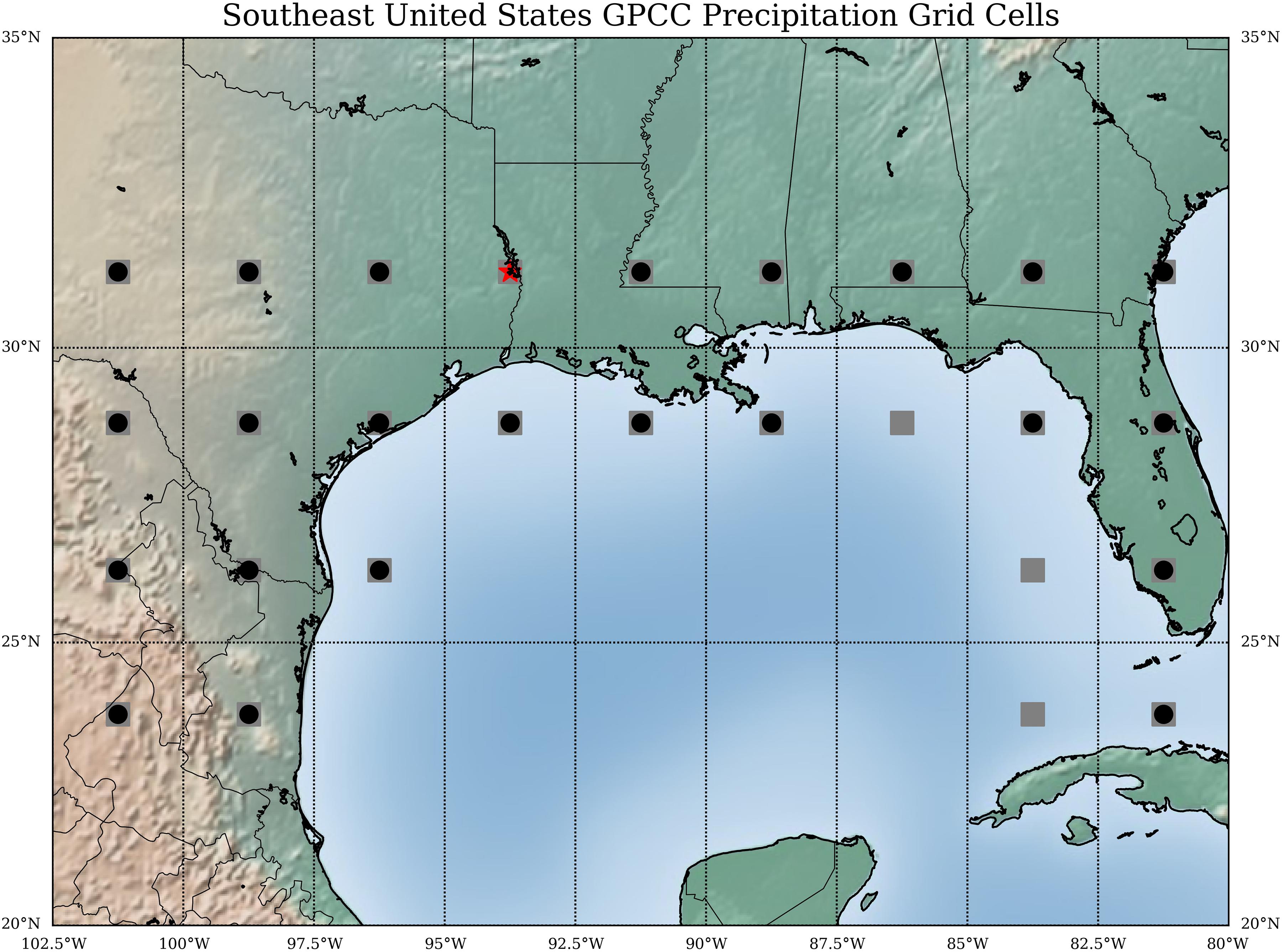
Figure 10. Mercator projection of the southeastern United States with superimposed markers indicating the center positions of the available 2.5-degree square grid cells spanning 22.5°N to 32.5°N and 102.5°W to 80.0°W. Gray squares are indicative of omitted grid cells while the red star denotes the grid cell concentrated on during the Gulf of Mexico wind component index case study.

Seasonal precipitation averages (mm/month) are calculated for each grid cell for the period 1910 - 2013 to gain a preliminary understanding of the interannual variability of precipitation across the region (Figure 11). The monthly temporal resolution of the GPCC precipitation dataset allows seasons to be easily categorized according to a common seasonal definition (Trenberth, 1983): winter (DJF), spring (March, April, and May; MAM), summer (June, July, and August; JJA), and fall (September, October, and November; SON). Since the dataset commences January 1910, the 1910 winter season average contains precipitation data only from January and February for that year. Five-, seven-, and nine-year running averages of the monthly precipitation are computed to draw out longer term signals (Figure 11) and reduce the noise inherent in rain data. This computation consequently also filters out large spatial scale interannual variability. For example, ENSO has been shown to influence the southeast United States’ interannual and inter-seasonal climate dynamics (Brown et al., 2019), and will not be captured with this temporal average. The 7-year running average provides a balance between the large variability in seasonal or annual precipitation averages and reduction of the signal due to smoothing; thus, the 7-year average will be used in the subsequent comparison to the Gulf of Mexico wind indices. The seasonal precipitation data are standardized using Eq. (6) to improve visual comparison to the directional wind index.

FIGURE 11

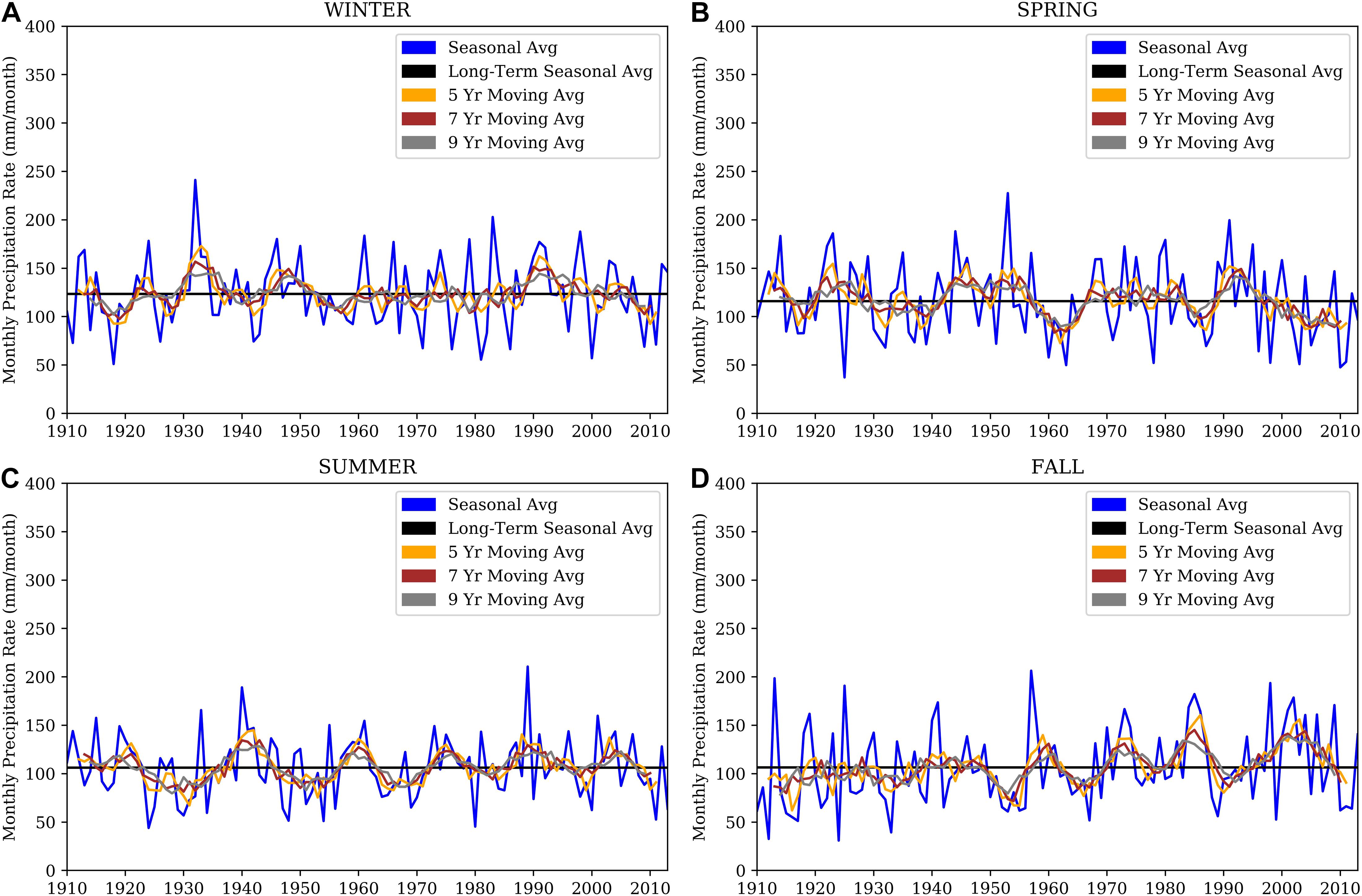
Figure 11. Time series of average seasonal precipitation rate (blue), long-term average seasonal precipitation rate (black), and 5-year (yellow), 7-year (red), and 9-year (gray) moving average seasonal precipitation rate for the grid cell centered on 31.25°N, 93.75°W (east Texas and southwest Louisiana). All plotted quantities for winter (A, top left), spring (B, top right), summer (C, bottom left), and fall (D, bottom right) have units of mm/month.

A preliminary analysis of the standardized 7-year running seasonal precipitation and wind indices reveals a decadal scale variability for several regions and seasons. The strongest relationships between winds and precipitation are apparent over Mexico, Texas, and Louisiana in the summer and fall seasons primarily after 1950, as represented by the standardized seasonal precipitation, meridional, and zonal wind indices for the grid cell centered at 31.25°N, 93.75°W (Figure 12). Generally, precipitation and the meridional wind index are in phase, while the zonal wind index is 180 degrees out of phase with respect to the other two indices. The magnitude of the summer and fall indices (Figures 12C,D) for the selected grid cell vary between -1.0 and 1.0. More specifically, the precipitation and meridional wind indices attained maxima, while the zonal wind index achieved a minimum. Across all locations and seasons along the Gulf Coast, the spatiotemporal relationship between the three indices becomes less clear prior to 1950. It is surmised that these discrepancies and weak connections may be explained by complications in data collection before and during World War II as well as less accurate rain gauge instrumentation. The signs and magnitudes of the respective component wind indices may be used to diagnose the synoptic flow and precipitation patterns. A positive (negative) seasonal meridional wind index correlates to a higher frequency of southerly (northerly) flow. Similarly, a positive (negative) seasonal zonal wind index represents a higher frequency of westerly (easterly) flow. The seasonal precipitation index is more straightforward in that a positive (negative) index translates to above (below) average precipitation.

FIGURE 12

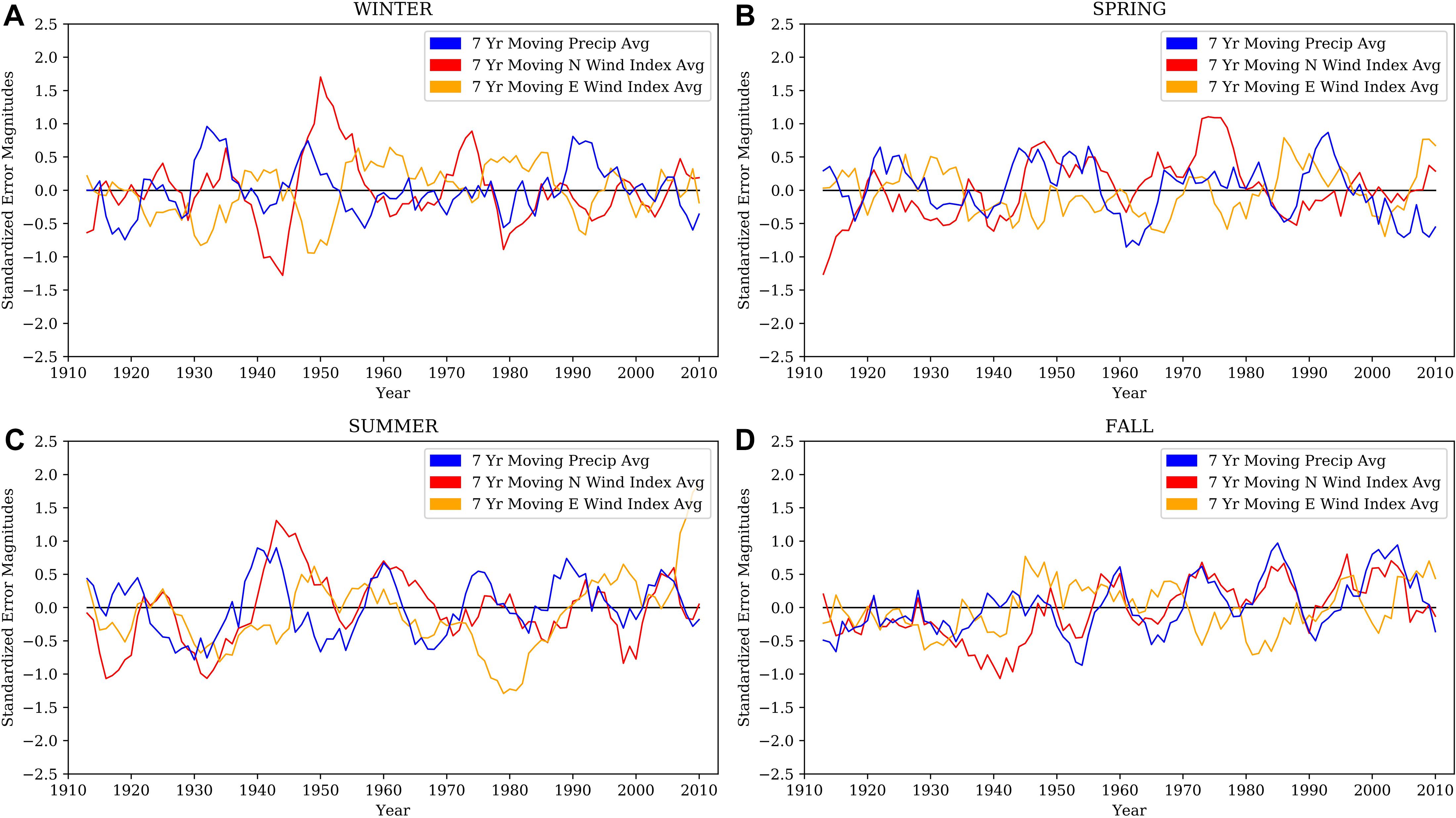
Figure 12. Time series of standardized 7-year moving average winter (A, top left), spring (B, top right), summer (C, bottom left), and fall (D, bottom right) precipitation rates (blue), northern wind component (red), and eastern wind component (yellow) for the grid cell 31.25°N, –93.75°W.

Since the grid cell representing eastern Texas/southwestern Louisiana (Figure 11) contains one of the strongest periodic signals, a multiple linear regression model is constructed to quantitatively assess the relationship between precipitation and wind components. Three regression models are applied to each season’s data based on the observed relationships pre- and post-1950: 1913–1949 (weak), 1950–2010 (strong), and all years (1913–2010). These regression lines are fit to the data such that the precipitation is a function of the zonal and meridional components and given by:

$P_{index}=M_1{N}_{index}+M_2{E}_{index}+C(9)$

where P_index is the predicted standardized precipitation index, M₁ and M₂ are the linear coefficients relating to the zonal standardized wind index (N_index) and the meridional standardized wind index (E_index), respectively, and C is an intercept coefficient. The seasonally generated multiple linear regression models for eastern Texas/southwestern Louisiana, including the regression curves, root-mean squared errors (RMSE) and coefficients of determination (r²) for the three periods superimposed on the seasonal precipitation series (Figure 13), quantify the wind index and precipitation relationships. Note that the post-1950 regression curve more closely follows the all-years regression curve as compared to the pre-1950 curve, which tends to deviate more from the all-years regression curve.

FIGURE 13

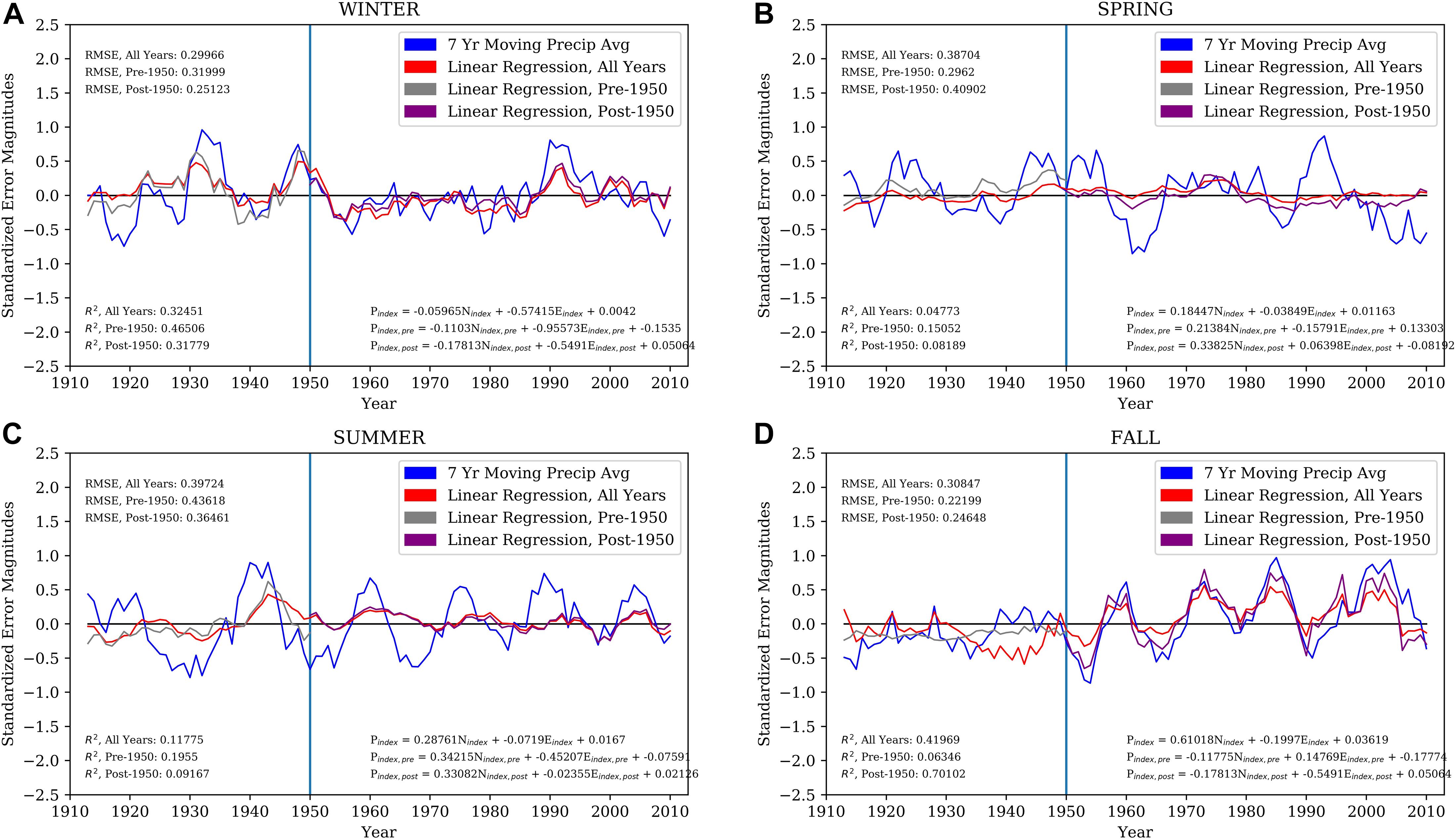
Figure 13. Time series of standardized 7-year moving average winter (A, top left), spring (B, top right), summer (C, bottom left), and fall (D, bottom right) precipitation rates (blue) and multiple linear regression models (text in bottom right in each panel) for all years (red), pre-1950 (gray), and post-1950 (purple). The root-mean-squared errors (RMSE) for these three regression curves are displayed in the top left and coefficients of determination (r²) in the bottom left in each panel.

While RMSE is a measure of how spread out the residuals (differences relative to the actual precipitation indices) are from the regression curves, r² is a better measure of goodness-of-fit as it explains how much variance in the observations can be explained by the linear regression, which is a function of season and location. During fall, stronger regional periodic changes in precipitation occur during post-1950 years in comparison to the weaker signals present in the pre-1950 examples (Figure 13). This is exhibited by the post-1950 years having a noticeably higher r² in contrast to that of the pre-1950 during the fall. The results from the fall season show that periods of more frequent northward (positive N_index) and westward (negative E_index) winds result in increased seasonal precipitation rates. Of the remaining seasons, winter exhibits the best goodness-of-fit from the regression curves, with the pre-1950 having the highest r²; however, the relationship between the zonal and meridional wind indices versus precipitation is not as obvious as for fall (Figure 12).

When we consider all the precipitation grids along the Gulf Coast, clear pattens of correlation between the wind component indices and precipitation appear (Figure 14). In the fall, two action centers appear between the r² pre- and post-1950 with one centered generally over the Texas/Louisiana border (near 30°N, 95°W) and the other over the Southeast/North Florida (near 30°N, 82.5°W). These action centers can be qualitatively associated with regions of less or more rainfall, with the precipitation patterns generally being stronger in the post-1950 period when the wind to precipitation r² are the largest. The authors note that although the association between wind indices and precipitation is strong in fall, this analysis is preliminary and additional analysis of the general circulation patterns (e.g., North Atlantic Oscillation, El Niño Southern Oscillation, and Pacific Decadal Oscillation) during each season is needed to better understand the observed wind-precipitation relationships. Datasets with higher resolution should be used to apply the aforementioned index methodologies and to conduct additional statistical analyses to observe potential smaller-scale features in the Gulf of Mexico and Atlantic Ocean.

FIGURE 14

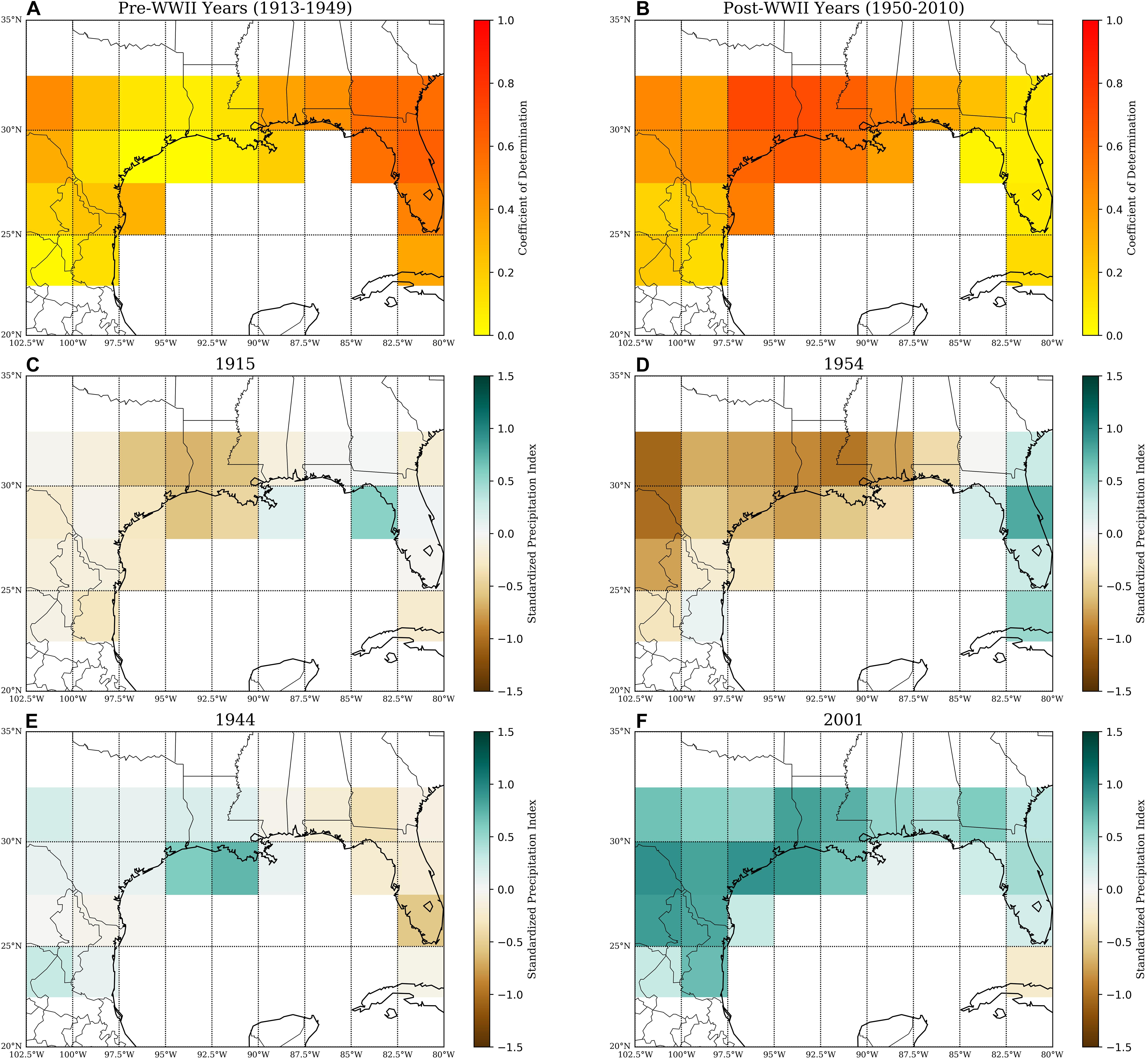
Figure 14. Map of coefficients of determination (r²) for the (A, top left) pre-1950 and (B, top right) post-1950 time periods. Standardized precipitation indices for the fall seasons of 1915 (C, middle left) and 1954 (D, middle right). These seasons were chosen to illustrate two fall seasons of below average precipitation for the 31.25°N, 93.75°W region. Standardized precipitation indices for the fall seasons of 1944 (E, bottom left) and 2001 (F, bottom right). These seasons were chosen to illustrate two fall seasons of above average precipitation for the 31.25°N, 93.75°W region.

Discussion and Future Work

Using ship-observed wind observations within ICOADS, the authors have successfully demonstrated a technique to create PDF-based wind component indices. The PDF approach differs from Wheeler et al. (2010) and Barriopedro et al. (2014) as follows: (1) the consideration of an increase in the eastward (northward) wind simultaneous with decreases in westward (southward) winds, which emphasizes shifts in a PDF more than increases in a specific cardinal direction; (2) that Wheeler et al.’s indices are based on changes in frequency of daily averaged winds, whereas we examine a distribution determined from spans of space and time; and (3) the addition of a time-varying uncertainty in the index. One benefit of this PDF approach over the Barriopedro et al. (2014) method is that this probabilistic index methodology is not limited to one specific variable. This method holds the ability to be applied to different variables and different datasets, which is being used in on going work by the authors for wind speed and pressure variables. By using a probabilistic approach to create the indices, the calculations are relatively insensitive to random error, as well as remaining independent of sample size for sufficiently large samples. An additional benefit is that these indices can be constructed for various regions and accumulation intervals, keeping in mind that the uncertainty in the index is directly related to the number of wind observations available. For this reason, the authors have chosen to create indices for the north Atlantic and eastern Gulf of Mexico that encompass the primary shipping routes, where observations are more frequent. Using only ship observations is recommended for century-scale wind indices because the addition of modern platforms (buoys, rigs, coastal stations) can result in artificial trends in the index (Figure 9B). However, if one was interested in creating modern era (e.g., post-1980) indices, using all platforms would increase the available observations and may provide additional insight into near-coastal wind variations if coastal station data were included.

There are advantages and challenges when working with historical marine observations (e.g., ICOADS). ICOADS is the most comprehensive, uniformly formatted marine dataset available with observations extending into the late 1600s (Freeman et al., 2017). This makes ICOADS ideal for long term climate studies. However, one must also be aware of the mix of data sources, varying observing platforms and sampling strategies through time (e.g., varying precision in directions), and the heterogeneous quality of wind observations. The quality control approaches applied to the ICOADS data by the authors represent only a cursory pass at excluding suspect observations. Additional quality control techniques, including comparison of near-neighboring ships or comparisons to satellite winds in the modern period, are likely to further exclude other ICOADS wind observations. Therefore, the variations shown in the north Atlantic and Gulf of Mexico wind component indices should be considered preliminary.

Regardless of these shortcomings with data quality assurance, the authors have shown that PDF-based wind component indices can be used as an indicator of previously observed climate phenomena (e.g., NAO) and can be used to identify relationships between marine wind and continental precipitation variability. Furthermore, the observational uncertainty in the example indices is small compared to the variability being examined, which indicates that the index is robust. For the Gulf of Mexico, the analysis provides a qualitative assessment of the spatiotemporal comparisons between precipitation and wind indices, but further research is needed to investigate the synoptic-scale dynamics in the Gulf and Caribbean. Work is presently ongoing to examine variations in the Bermuda High and lower tropospheric circulation patterns over the tropical Atlantic, Caribbean, and Gulf of Mexico, which should shed light on how the lower-atmospheric circulation is varying as indicated by high and low phases of the eastern Gulf of Mexico component indices. This future analysis may reveal indications of changes in lower tropospheric circulation over the Gulf and Caribbean after 1980 that is correlated to the upward trend toward more frequent eastward winds and to the precipitation variability shown in the preliminary analysis along the Gulf Coast.

Data Availability Statement

Publicly available datasets were analyzed in this study. This data can be found here: https://doi.org/10.5065/D6ZS2TR3, https://climatedataguide.ucar.edu/climate-data/hurrell-north-atlantic-oscillation-nao-index-pc-based, https://doi.org/10.7289/V5C8276M, and https://doi.org/10.5194/essd-5-71-2013.

Author Contributions

SS, RR, JS, HM, and MB all contributed to the text, figures, and tables included in this manuscript. All authors contributed to the article and approved the submitted version.

Funding

This study was supported by NOAA’s Climate Program Office, Climate Monitoring Program under grant NA17OAR4310153.

Conflict of Interest

The authors declare that the research was conducted in the absence of any commercial or financial relationships that could be construed as a potential conflict of interest.

Acknowledgments

The authors acknowledge the contributions from the Marine Data Center programming team including Jocelyn Elya, E. Michael McDonald, and a number of undergraduate students that assisted in developing the ICOADS database and data analysis tools used to complete this research.

References

Amante, C., and Eakins, B. W. (2009). ETOPO1 1 Arc−Minute Global Relief Model: Procedures, Data Sources and Analysis. NOAA Technical Memorandum NESDIS NGDC−24. National Geophysical Data Center, NOAA, doi: 10.7289/V5C8276M [2 November 2020].

CrossRef Full Text | Google Scholar

American Meteorological Society. (2000). Glossary of Meteorology, 2nd Edn, ed. T. S. Glickman (American Meteorological Society), 855.

Google Scholar

Barriopedro, D., Gallego, D., Alvarez-Castro, M. C., García-Herrera, R., Wheeler, D., Peña-Ortiz, C., et al. (2014). Witnessing North Atlantic westerlies variability from ships’ logbooks (1985-2008). Clim. Dyn. 43, 939–955. doi: 10.1007/s00382-013-1957-8

CrossRef Full Text | Google Scholar

Becker, A., Finger, P., Meyer-Christoffer, A., Rudolf, B., Schamm, K., Schneider, U., et al. (2013). A description of the global land-surface precipitation data products of the Global Precipitation Climatology Centre with sample application including centennial (trend) analysis from 1901–present. Earth Syst. Sci. Data 5, 71–99. doi: 10.5194/essd-5-71-2013

CrossRef Full Text | Google Scholar

Berry, D. I., and Kent, E. C. (2011). Air-sea fluxes from ICOADS: the construction of a new gridded dataset with uncertainty estimates. Int. J. Climatol. 31, 987–1001. doi: 10.1002/joc.2059

CrossRef Full Text | Google Scholar

Bourassa, M. A., Romero, R., Smith, S. R., and O’Brien, J. J. (2005). A new FSU wind climatology. J. Climate 18, 3692–3704.

Google Scholar

Brown, V. M., Keim, B. D., and Black, A. W. (2019). Climatology and Trends in Hourly Precipitation for the Southeast United States. J. Hydrometeor 20, 1737–1755. doi: 10.1175/JHM-D-19-0004.1

CrossRef Full Text | Google Scholar

Climate Analysis Section. (2003). Hurrell North Atlantic Oscillation (Nao) Index (Pc-Based). Available online at: https://climatedataguide.ucar.edu/climate-data/hurrell-north-atlantic-oscillation-nao-index-pc-based (accessed September 23, 2020).

Google Scholar

Cook, E. R., D’Arrigo, R. D., and Mann, M. E. (2002). A well-verified, multiproxy reconstruction of the winter North Atlantic Oscillation index since A.D. 1400. J. Clim 15, 1754–1764. doi: 10.1175/1520-04422002015<1754:AWVMRO<2.0.CO;2

CrossRef Full Text | Google Scholar

Cook, E. R., Kushnir, Y., Smerdon, J. E., Williams, A. P., Anchukaitis, K. J., and Wahl, E. R. (2019). A Euro-Mediterranean tree-ring reconstruction of the winter NAO index since 910 C.E. Clim. Dyn. 53, 1567–1580. doi: 10.1007/s00382-019-04696-2

CrossRef Full Text | Google Scholar

Fairbanks, R. G., Evans, M. N., Rubenstone, J. L., Mortlock, R. A., Broad, K., Moore, M. D., et al. (1997). Evaluating climate indices and their geochemical proxies measured in corals. Coral Reefs. 16, 93–100. doi: 10.1007/s003380050245

CrossRef Full Text | Google Scholar

Freeman, E., Woodruff, S. D., Worley, S. J., Lubker, S. J., Kent, E. C., Angel, W. E., et al. (2017). ICOADS Release 3.0: a major update to the historical marine climate record. Int. J. Climatol. 37, 2211–2232. doi: 10.1002/joc.4775

CrossRef Full Text | Google Scholar

García-Herrera, R., Können, G. P., Wheeler, D. A., Prieto, M. R., Jones, P. D., and Koek, F. B. (2005). CLIWOC: A Climatological Database for the World’s Oceans 1750-1854. Climatic Change 73, 1–12. doi: 10.1007/s10584-005-6952-6

CrossRef Full Text | Google Scholar

García-Herrera, R., Barriopedro, D., Gallego, D., Mellado−Cano, J., Wheeler, D., and Wilkinson, C. (2018). Understanding weather and climate of the last 300 years from ships’ logbooks. WIREs Clim Change 9, e544. doi: 10.1002/wcc.544

CrossRef Full Text | Google Scholar

Gershunov, A., and Barnett, T. P. (1998). ENSO Influence on Intraseasonal Extreme Rainfall and Temperature Frequencies in the Contiguous United States: Observations and Model Results. J. Clim 11, 1575–1586. doi: 10.1175/1520-04421998011<1575:EIOIER<2.0.CO;2

CrossRef Full Text | Google Scholar

Hanley, D. E., Bourassa, M. A., O’Brien, J. J., Smith, S. R., and Spade, E. R. (2003). A quantitative evaluation of ENSO indices. Journal of Climate 16, 1249–1258.

Google Scholar

Hurrell, J. W. (1995). Decadal trends in the North Atlantic oscillation: Regional temperatures and precipitation. Science. 269, 676–679. doi: 10.1126/science.269.5224.676

PubMed Abstract | CrossRef Full Text | Google Scholar

Hurrell, J. W., and Deser, C. (2010). North Atlantic climate variability: The role of the North Atlantic Oscillation. J. Mar. Syst. 79, 231–244. doi: 10.1016/j.jmarsys.2009.11.002

CrossRef Full Text | Google Scholar

Hurrell, J. W., Kushnir, Y., Ottersen, G., and Visbeck, M. (2003). The North Atlantic Oscillation: climatic significance and environmental impact. Geophysical Monograph, Vol. 134. Washington, D.C: American Geophysical Union, doi: 10.1029/GM134

CrossRef Full Text | Google Scholar

Laplace, P. S. (1812). Théorie analytique des probabilités (in French). Ve. Courcier. 283.

Google Scholar

Larkin, N. K., and Harrison, D. E. (2005). On the definition of El Niño and associated seasonal average U.S. weather anomalies. Geophys. Res. Lett. 32, L13705. doi: 10.1024/2005GL022738

CrossRef Full Text | Google Scholar

L’Heureux, M. L., Tippett, M. K., and Barnston, A. G. (2015). Characterizing ENSO Coupled Variability and Its Impact on North American Seasonal Precipitation and Temperature. Journal of Climate 28, 4231–4245. doi: 10.1175/JCLI-D-14-00508.1

CrossRef Full Text | Google Scholar

Lindau, R. (1995). “A new Beaufort equivalent scale,” in Proceedings of the International COADS Winds Workshop, Kiel, (Germany: Institutfür Meereskunde Kiel and NOAA), 232–252.

Google Scholar

Luterbacher, J., Xoplaki, E., Dietrich, D., Rickli, R., Jacobeit, J., Beck, C., et al. (2002). Reconstruction of sea level pressure fields over the Eastern North Atlantic and Europe back to 1500. Clim. Dyn. 18, 545–562. doi: 10.1007/s00382-001-0196-6

CrossRef Full Text | Google Scholar

Mann, M. E., Zhang, Z., Hughes, M. K., Bradley, R. S., Miller, S. K., Rutherford, S., et al. (2008). Proxy-based reconstructions of hemispheric and global surface temperature variations over the past two millennia. Proc. Natl. Acad. Sci. U. S. A. 105, 13252–13257. doi: 10.1073/pnas.0805721105

PubMed Abstract | CrossRef Full Text | Google Scholar

Mo, K. C., Schemm, J. E., and Yoo, S. (2009). Influence of ENSO and the Atlantic Multidecadal Oscillation on Drought over the United States. Journal of Climate 22, 5962–5982. doi: 10.1175/2009JCLI2966.1

CrossRef Full Text | Google Scholar

NOAA. (2016). International Comprehensive Ocean-Atmosphere Data Set, Release 3.0, Quality control (QC) and related processing. 15. Available online at: https://icoads.noaa.gov/e-doc/R3.0-stat_trim.pdf (accessed November 2, 2020).

Google Scholar

Pinto, J. G., and Raible, C. C. (2012). Past and Recent Changes in the North Atlantic Oscillation. Wiley Interdiscip. Rev. Climate Change 3, 79–90. doi: 10.1002/wcc.150

CrossRef Full Text | Google Scholar

Research Data Archive, Computational and Information Systems Laboratory, National Center for Atmospheric Research, University Corporation for Atmospheric Research, and Coauthors, et al. (2016). International Comprehensive Ocean-Atmosphere Data Set (ICOADS) Release 3, Individual Observations. Research Data Archive at the National Center for Atmospheric Research. Boulder, CO: Computational and Information Systems Laboratory, doi: 10.5065/D6ZS2TR3 [Database copy provided to FSU/COAPS in November 2017].

CrossRef Full Text | Google Scholar

Rogers, J. C. (1997). North Atlantic storm track variability and its association to the North Atlantic oscillation and climate variability of Northern Europe. J. Clim 10, 1635–1647. doi: 10.1175/1520-04421997010<1635:NASTVA<2.0.CO;2

CrossRef Full Text | Google Scholar

Ropelewski, C. F., and Halpert, M. S. (1986). North American Precipitation and Temperature Patterns Associated with the El Niño/South Oscillation (ENSO). Mon. Wea. Rev 114, 2352–2362. doi: 10.1175/1520-04931986114<2352:NAPATP<2.0.CO;2

CrossRef Full Text | Google Scholar

Ropelewski, C. F., and Jones, P. D. (1987). An Extension of the Tahiti-Darwin Southern Oscillation Index. Mon. Wea. Rev 115, 2161–2165. doi: 10.1175/1520-04931987115<2161:AEOTTS<2.0.CO;2

CrossRef Full Text | Google Scholar

Serreze, M. C., Carse, F., Barry, R. G., and Rogers, J. C. (1997). Icelandic low cyclone activity: Climatological features, linkages with the NAO, and relationships with recent changes in the Northern Hemisphere circulation. J. Clim 10, 453–464. doi: 10.1175/1520-04421997010<0453:ILCACF<2.0.CO2

CrossRef Full Text | Google Scholar

Slutz, R. J., Lubker, S. J., Hiscox, J. D., Woodruff, S. D., Jenne, R. L., Joseph, D. H., et al. (1985). Comprehensive Ocean-Atmosphere Data Set; Release 1. Boulder, CO: NOAA Environmental Research Laboratories, Climate Research Program, 268. (NTIS PB86-105723).

Google Scholar

Smith, S. R., Bourassa, M. A., and Sharp, R. J. (1999). Establishing more truth in true winds. J. Atmos. Oceanic Technol. 16, 939–952.

Google Scholar

Smith, S. R., Briggs, K., Bourassa, M. A., Elya, J., and Paver, C. R. (2018). Shipboard automated meteorological and oceanographic system data archive: 2005–2017. Geosci Data J 5, 73–86. doi: 10.1002/gdj3.59

CrossRef Full Text | Google Scholar

Smith, S. R., Freeman, E., Lubker, S. J., Woodruff, S. D., Worley, S. J., Angel, W. E., et al. (2016). The International Maritime Meteorological Archive (IMMA) format. Available online at: http://icoads.noaa.gov/e-doc/imma/R3.0-imma1.pdf (accessed August 20, 2020)

Google Scholar

Smith, S. R., Hughes, P. J., and Bourassa, M. A. (2011). A comparison of nine monthly air–sea flux products. International Journal of Climatology 31, 1002–1027.

Google Scholar

Smith, S. R., Servain, J., Legler, D. M., Stricherz, J. N., Bourassa, M. A., and O’Brien, J. J. (2004). In Situ-Based Pseudo-Wind Stress Products for the Tropical Oceans. Bull. Am. Meteorol. Soc. 85, 979–994. doi: 10.1175/BAMS-85-7-979

CrossRef Full Text | Google Scholar

Thomas, B. R., Kent, E. C., and Swail, V. R. (2005). Methods to homogenize with speeds from ships and buoys. Int. J. Climatol. 25, 979–995. doi: 10.1002/joc.1176

CrossRef Full Text | Google Scholar

Trenberth, K. E. (1983). What are the seasons? Bull. Amer. Meteor. Soc 64, 1276–1282. doi: 10.1175/1520-04771983064<1276:WATS<2.0.CO;2

CrossRef Full Text | Google Scholar

van Loon, H., and Madden, R. A. (1981). The Southern Oscillation. Part I: Global associations with pressure and temperature in northern winter. Monthly Weather Review 109, 1150–1162.

Google Scholar

Wheeler, D. (2004). Understanding seventeeth-century ships’ logbooks: An exercise in historical climatology. J. Marit. Res. 6, 21–36. doi: 10.1080/21533369.2004.9668335

CrossRef Full Text | Google Scholar

Wheeler, D., García-Herrera, R., Wilkinson, C. W., and Ward, C. (2010). Atmospheric circulation and storminess derived from Royal Navy logbooks: 1685 to 1750. Clim. Change 101, 257–280. doi: 10.1007/s10584-009-9732-x

CrossRef Full Text | Google Scholar

Wheeler, D., and Wilkinson, C. (2004). From calm to storm: the origins of the Beaufort wind scale. The Mariner’s Mirror 90, 187–201.

Google Scholar

Wilson, R., Cook, E., D’Arrigo, R., Riedwyl, N., Evans, M. N., Tudhope, A., et al. (2010). Reconstructing ENSO: the influence of method, proxy data, climate forcing and teleconnections. J. Quat. Sci. 25, 62–78. doi: 10.1002/jqs.1297

CrossRef Full Text | Google Scholar

Woodruff, S. D. (2007). “Archival of data other than in IMMT format: the International Maritime Meteorological Archive (IMMA) format,” in proceedings of the Second Session of the JCOMM Expert Team on Marine Climatology (ETMC), Geneva, Switzerland, 26-27 March 2007. JCOMM Meeting Report No. 50, 68-101, (Geneva).

Google Scholar