Seafloor Density Contrast Derived From Gravity and Shipborne Depth Observations: A Case Study in a Local Area of Atlantic Ocean

Introduction

Shallow seabed density information plays an important role in understanding submarine structure, mineral exploration, military activity, and scientific research (Nagendra et al., 1996; Felix et al., 2002; Hsiao et al., 2011; Sandwell et al., 2014a). For a local ocean area, the shipborne equipment can be used for the detection. However, for the global ocean area, it is very difficult to detect and retrieve the shallow seabed density distribution with high resolution and high precision using ship-borne observations.

Currently, there are mainly two methods for the study of the Earth’s internal structure, including the density contrast of the seabed, i.e., the density difference between the seawater and the upper crust. One is based on seismic wave data and the other is based on gravity data. For the former, scholars have carried out a lot of investigations. For example, Soller et al. (1982) derived a global crustal thickness model with resolution of 2° × 2° based on seismic data; Nataf and Ricard (1996) combined geothermal and seismic data to invert the density structure of the global and upper mantle; Mooney et al. (1998) published a global crustal model crush with a spatial resolution of 5° × 5°. Based on seismic, ice sheet and sedimentary datasets, Bassin (2000) derived the crustal model CRUST2.0 with a resolution of 2° × 2° and Laske et al. (2013) released the crustal model CRUST1.0 with a spatial resolution of 1° × 1° based on CRUST5.1 and CRUST2.0. The above models provide not only the thickness information of each layer, including water layer, ice layer, soft sedimentary layer, hard sedimentary layer, upper crust, middle and lower crust, but also the density information. These models play a significant role in the study of the Earth’s internal structure.

However, the above models cannot fully meet all the application requirements. For example, the spatial resolution of the global model published only reaches 100 km, which is obviously insufficient for studying many local problems. In addition, the models mentioned above have great uncertainties in many regions, mainly because of the uneven distribution of seismic observation stations, and thus there are no or few seismic observations in some regions. Therefore, if one wants to retrieve the density distribution of the Earth’s interior with higher spatial resolution using information from seismic data, a densification of current network of seismic stations is needed. It would involve a lot of financial and material resources.

Another method is to use gravity field data for density inversion. Many algorithms for inversion of the Earth’s internal structure or density distribution using gravity data have been proposed and adopted. Parker (1972) gave the Fourier relationship between the depth of density interface and gravity anomaly in frequency domain. According to the relationship, the depth of density interface can be deduced from gravity anomaly. The related formula has been widely used in inversion of Moho surface depth and seafloor topography, such as Jiang et al. (2015); Hu et al. (2015), and Sandwell et al. (2014a), etc. Indeed, the formula is based on the premise that there is a density anomaly and the density contrast is known. Conversely, if the depth of the density interface is known, the formula can also be used to derive the density contrast. In recent years, with the emergence of new altimetry technologies and the release of new altimetry satellite products, Sandwell et al. (2014a) studied the submarine structure, especially using the gravity gradient data to find and confirm the position of the plate boundary on the seabed, which can also be regarded as a density interface.

Definitely, gravity data can be used to detect the density distribution of the Earth’s interior. However, some problems exist in the study of the Earth’s interior structure (including the density contrast of the seabed) using gravity data. For example, the inversion results are usually not unique. The fundamental reason is that many sources of gravity anomaly information exist, including not only the seabed density contrast, but also the depth of the density interface (that is, the ocean depth). Therefore, if we can combine the ocean gravity field and the ocean depth information well, it is possible to retrieve the seabed density contrast information with high accuracy.

Indeed, in the inversion of seafloor topography, many methods have been proposed for density contrast determination, such as the iterative search method (Kim et al., 2011; Ouyang et al., 2014; Xiang et al., 2017). However, the density contrast derived in the bathymetry inversion usually have no physical meaning (Annan and Wan, 2020), since the purpose of these researches is to inverse bathymetry. The idea of this study is to take the density contrasts of the seabed as the inversion product while the water depths are known.

With the advances in space technology, highly accurate marine gravity anomaly products (Hwang et al., 2002; Andersen et al., 2010; Hwang and Chang, 2014; Sandwell et al., 2014b; Zhu et al., 2020) with resolution of 1′ × 1′ have been derived using satellite altimetry observations. Besides gravity field data, a large amount of shipborne depths have been obtained by many years of ship sounding observations. It is roughly estimated that NOAA (National Oceanic and Atmospheric Administration) has collected more than 50 million shipborne depth observations. Therefore, it is possible to achieve good results by making full use of the shipborne sounding data and gravity data to jointly invert the seabed density contrast. This study presents a case study. Section “Materials and Methods” introduces the inversion algorithm. Study area and data are described in section “Study Area and Data. Results and analysis are presented in section “Results and Analysis” and conclusions are derived finally in section “Conclusion.”

Materials and Methods

Function Model

According to principle of the gravity geological method (GGM) (Ibrahim and Hinze, 1972), we have:

$${\widehat{g}}_i=2\mathrm{\pi }G\mathrm{\Delta }\widehat{\mathrm{\rho }}(H-{\widehat{h}}_i)+{\widehat{g}}_l(1)$$

where ${\widehat{g}}_i$ denotes the gravity anomaly observation at the i^th point; ${\widehat{g}}_l$ denotes the long wavelength part of the gravity anomaly; G means the gravitational constant; Δρ represents the density contrast; H is the depth datum and ${\widehat{h}}_i$ denotes the water depths at the i^th points. Definitely, the gravity anomaly observations have a linear relationship with $(H-\widehat{h})$. In a local small area, the long wavelength part of gravity anomaly ${\widehat{g}}_l$ and density contrast $\mathrm{\Delta }\widehat{\mathrm{\rho }}$ can be seen as constants. Hence, Equation 1 can be rewritten as:

$${\widehat{g}}_i=\left[\begin{array}{c}\hfill {\widehat{g}}_1\hfill \\ \hfill {\widehat{g}}_2\hfill \\ \hfill {\widehat{g}}_3\hfill \\ \hfill \mathrm{⋮}\hfill \\ \hfill {\widehat{g}}_n\hfill \end{array}\right]=\left[\begin{array}{cc}\hfill 1\hfill & \hfill 2\mathrm{\pi }G(H-{\widehat{h}}_1)\hfill \\ \hfill 1\hfill & \hfill 2\mathrm{\pi }G(H-{\widehat{h}}_2)\hfill \\ \hfill 1\hfill & \hfill 2\mathrm{\pi }G(H-{\widehat{h}}_3)\hfill \\ \hfill \mathrm{⋮}\hfill & \hfill \mathrm{⋮}\hfill \\ \hfill 1\hfill & \hfill 2\mathrm{\pi }G(H-{\widehat{h}}_n)\hfill \end{array}\right]\left[\begin{array}{c}\hfill {\widehat{g}}_l\hfill \\ \hfill \mathrm{\Delta }\widehat{\mathrm{\rho }}\hfill \end{array}\right](2)$$

Because both gravity anomaly and water depth datasets contain noises, two types of data error should be considered in the determination of the density contrast $\mathrm{\Delta }\widehat{\mathrm{\rho }}$ and long wavelength of gravity anomaly ${\widehat{g}}_l$. Ordinary least squares method only considers the error of dependent variable, i.e., gravity anomaly errors and ignores the error of bathymetric data measured by ships. Hence, the inversion result by traditional least squares method based on Equation 2 would be not accurate enough. Instead, the total least squares (TLS) (Golub and van Loan, 1980; Xu et al., 2012) method was adopted in this study. Considering the two types of observation errors, the following equation can be constructed:

$${\widehat{g}}_i+v_{gi}=2\mathrm{\pi }G\mathrm{\Delta }\widehat{\mathrm{\rho }}(H-h_i-v_{hi})+{\widehat{g}}_l(3)$$

In which, v_gi and v_hi are the noises of gravity anomaly and shipborne depths respectively. Changing Equation 3 into the form of EIV (error in variables) model results in:

$$\left(A+E_A\right)x=L+E_L(4)$$

where A is the coefficient matrix; E_A,E_L are the errors of matrices of A and observation vector L; x is the parameter to be estimated, i.e.,

$$\begin{array}{c}A=\left[\begin{array}{cc}\hfill 1H-h_1\hfill & \\ \hfill 1H-h_2\hfill & \\ \hfill \mathrm{⋮}\mathrm{⋮}\hfill & \\ \hfill 1H-h_3\hfill & \end{array}\right]E_A=\left[\begin{array}{cc}\hfill 0v_{h1}\hfill & \\ \hfill 0v_{h2}\hfill & \\ \hfill \mathrm{⋮}\mathrm{⋮}\hfill & \\ \hfill 0v_{h3}\hfill & \end{array}\right]\hfill \\ x=\left[\begin{array}{c}\hfill {\widehat{g}}_l\hfill \\ \hfill 2\mathrm{\pi }G\mathrm{\Delta }\widehat{\mathrm{\rho }}\hfill \end{array}\right]L=\left[\begin{array}{c}\hfill g_1\hfill \\ \hfill g_2\hfill \\ \hfill \mathrm{⋮}\hfill \\ \hfill g_n\hfill \end{array}\right]E_L=\left[\begin{array}{c}\hfill v_{g1}\hfill \\ \hfill v_{g2}\hfill \\ \hfill \mathrm{⋮}\hfill \\ \hfill v_{gn}\hfill \end{array}\right]\hfill \end{array}(5)$$

The final solution can be derived by the following rule.

$$v_s{v}_s^{\text{T}}=\sum _{i=1}^n{v}_{hi}^2+\sum _{i=1}^n{v}_{gi}^2=\min (6)$$

Solution of TLS

Solution of the TLS can be derived by Singular Value Decomposition (SVD) (Golub and van Loan, 1980). Firstly, augmented matrix C is defined as:

$$C=\left[AL\right]=\left[\begin{array}{ccc}\hfill 1\hfill & \hfill H-h_1\hfill & \hfill g_1\hfill \\ \hfill 1\hfill & \hfill H-h_2\hfill & \hfill g_2\hfill \\ \hfill \mathrm{⋮}\hfill & \hfill \mathrm{⋮}\hfill & \hfill \mathrm{⋮}\hfill \\ \hfill 1\hfill & \hfill H-h_n\hfill & \hfill g_n\hfill \end{array}\right](7)$$

And then Orthogonal Trigonometric (QR) decomposition is conducted on matrix C, in which Q is the orthogonal matrix as follows:

$$C=QR(8)$$

$$R=Q^{-1}C=Q^{\text{T}}C=\left[\begin{array}{ccc}\hfill R_{11}\hfill & \hfill R_{12}\hfill & \hfill R_{1l}\hfill \\ \hfill 0\hfill & \hfill R_{22}\hfill & \hfill R_{2l}\hfill \end{array}\right]\begin{array}{c}\hfill n\hfill \\ \hfill n-m\hfill \end{array}(9)$$

Based on the singular value decomposition of R-part of matrix C_R, the solution of TLS is obtained as Equation 10:

$$C_R=\left[R_{22}{R}_{2l}\right]=U•\sum •V^{\text{T}}(10)$$

where ∑ = diag(δ₁,δ₂) with singular values δ₁≥δ₂≥0. And thus, the estimated parameters can be derived by the following equation.

$$\left[\begin{array}{c}\hfill \widehat{a}\hfill \\ \hfill \widehat{b}\hfill \end{array}\right]=\left[\begin{array}{c}\hfill 2\mathrm{\pi }G\mathrm{\Delta }\widehat{\mathrm{\rho }}\hfill \\ \hfill g_l\hfill \end{array}\right]={\left(A{A}^{\text{T}}-{\mathrm{\delta }}_2^2\left[\begin{array}{cc}\hfill 0\hfill & \hfill 0\hfill \\ \hfill 0\hfill & \hfill 1\hfill \end{array}\right]\right)}^{-1}{A}^{\text{T}}l(11)$$

Finally, we have:

$$\mathrm{\Delta }\widehat{\mathrm{\rho }}=\frac{\widehat{a}}{2\mathrm{\pi }G}(12)$$

The accuracy of TLS solution is evaluated by standard deviation of unit weight (SDUW) as follows:

$${\mathrm{\delta }}_{tls}=\sqrt{\frac{v_s{v}_s^{\text{T}}}{n-2}}(13)$$

where $v_s{v}_s^T=v_x{v}_x^T+v_y{v}_y^T$.

Filtering Method

In order to test the sensitive band of gravity anomaly to the seafloor topography, which is the basis for deriving the density contrast, band filtering with different pass bands was experimented and the correlation analysis was conducted correspondingly. The band-pass filters proposed by Smith and Sandwell (1994), which is indeed a filter by combining a Gaussian high-pass filter and a Wiener low-pass filter was used. According to Smith and Sandwell (1994), the high-pass filter is defined as Equation 14:

$$w_1(k)=1-e^{-2{\left(\mathrm{\pi }ks\right)}^2}(14)$$

where $k=\frac{1}{\mathrm{\lambda }}$, λ denotes the wavelength; s is a parameter of the filter which can be derived by w_l(k) = 0.5 at the cutoff wavelength (denoted as λ_h):

$$s=\frac{{\mathrm{\lambda }}_h\sqrt{2\ln 2}}{2\mathrm{\pi }}(15)$$

The low-pass filter is defined as Equation 16:

$$w_l(k)={\left(1+\mathrm{A}{k}^4{e}^{4\mathrm{\pi }kd}\right)}^{-1}(16)$$

where d is the mean depth of the study area; A is parameter of the filter, which can be derived by w_l(k) = 0.5 at the cutoff wavelength (denoted as λ_l) as:

$$A={\mathrm{\lambda }}_l^4{e}^{-\frac{4\mathrm{\pi }d}{{\mathrm{\lambda }}_l}}(17)$$

Finally, the bandpass filter is obtained as:

$$w=w_h{(k)}^{*}{w}_l(k)(18)$$

Study Area and Data

Study Area and Observation Data

The study area is a local region in the Atlantic Ocean, i.e., 326°E-328°E, 3.5°N–4.5°N. The bathymetric data from ship survey were provided by First Institute of Oceanography, Ministry of Nature Resources, and 498,501 shipborne depths are obtained by multibeam echo-sounding with high accuracy. The gravity data used is DTU13 version of gravity anomaly model released by Technical University of Denmark¹. DTU13 is derived based on DTU10 by adding more satellite observations, such as Cryosat-2 (Andersen et al., 2014). The resolution of DTU13 is 1′ × 1′ and its precision is better than four mGal (Andersen, 2010; Andersen et al., 2014).

The whole study area is divided into eight small areas, denoted as A, B, C, D, E, F, G, and H with at a size of 30′×30′, as shown in Figure 1, in which water depths are shown by different colors. The three-dimensional distributions of gravity anomaly and shipborne depths are shown in Figure 2. According to this figure, the two maps show very similar characteristics which denote the high correlation between the two types of datasets.

FIGURE 1

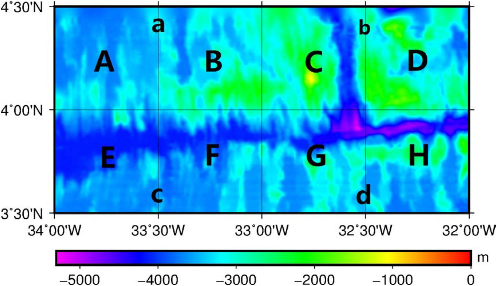
Figure 1. Bathymetry of study area.

FIGURE 2

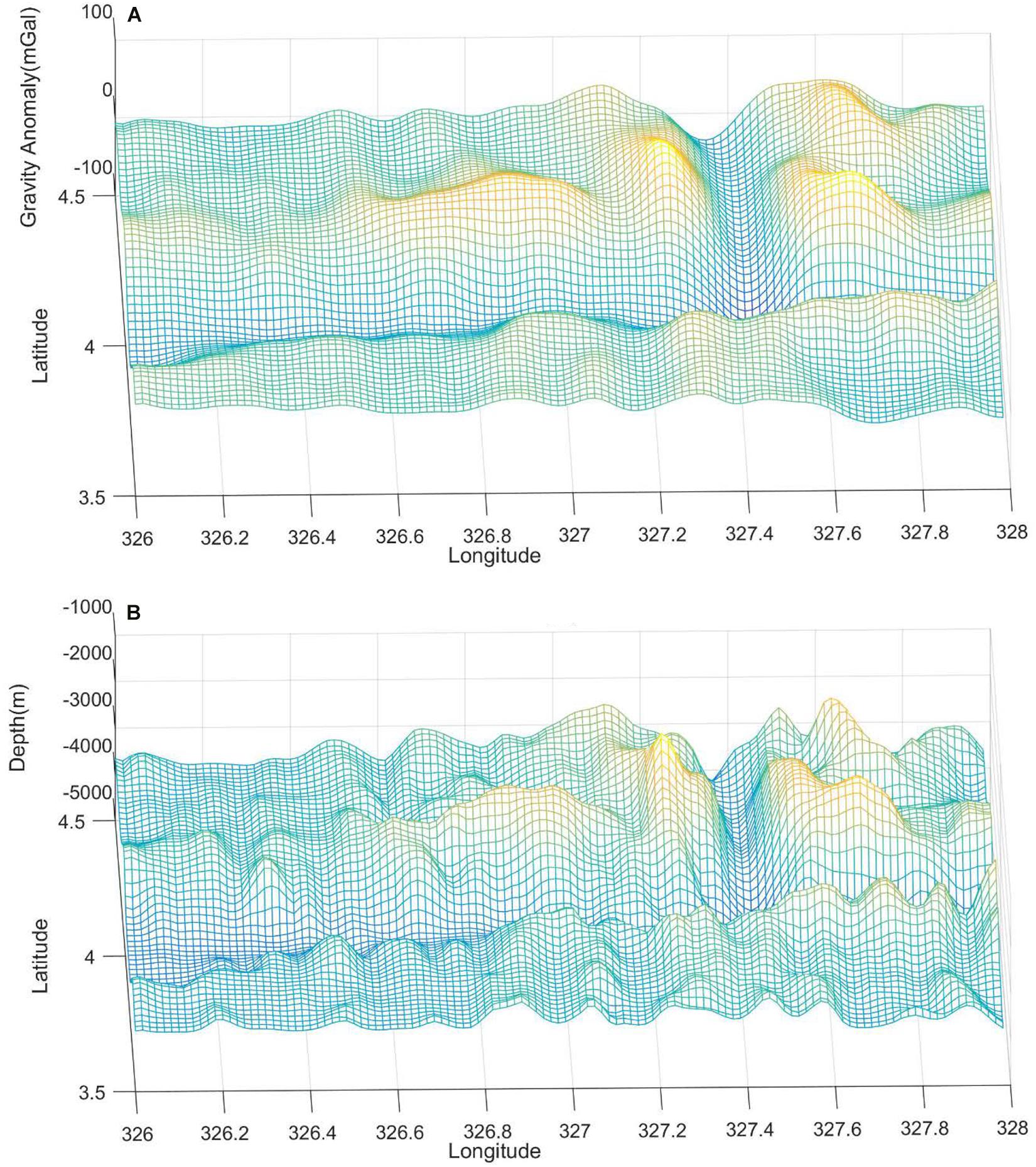
Figure 2. Three-dimensional distribution of gravity anomaly (A) and shipborne depths (B).

Density Contrast From CRUST 1.0

CRUST1.0, the latest crustal model with a resolution of 1° × 1°, is used for comparisons. It provides density information of seven layers, including water layer, ice layer, soft sedimentary layer, hard sedimentary layer, upper crust, middle crust, and lower crust. In this model, the Earth is divided into 64,800 units and each unit has a size of 1° × 1°. Sea water depth, crustal thickness, and density are derived by the average data in each unit.

Considering that the spatial resolution of CRUST1.0 is 1° × 1° and the size of the study area is 1° × 2°, only four density contrasts were derived using CRUST1.0 in the study area, for four regions defined as a, b, c, and d corresponding to A and B, C and D, E and F, and G and H shown in Figure 1 respectively. Parameters of CRUST1.0 in each region are presented in Table 1, in which the density contrast $\mathrm{\Delta }{\overline{\mathrm{\rho }}}_0$ is the difference between sea water and the upper crust. It is found that the four density contrasts are almost same except in area CD. According to Table 1, the thickness of the upper crust in region CD is largest compared to other regions. This may cause the differences in the density contrasts with other region, which would be investigated in future research.

TABLE 1

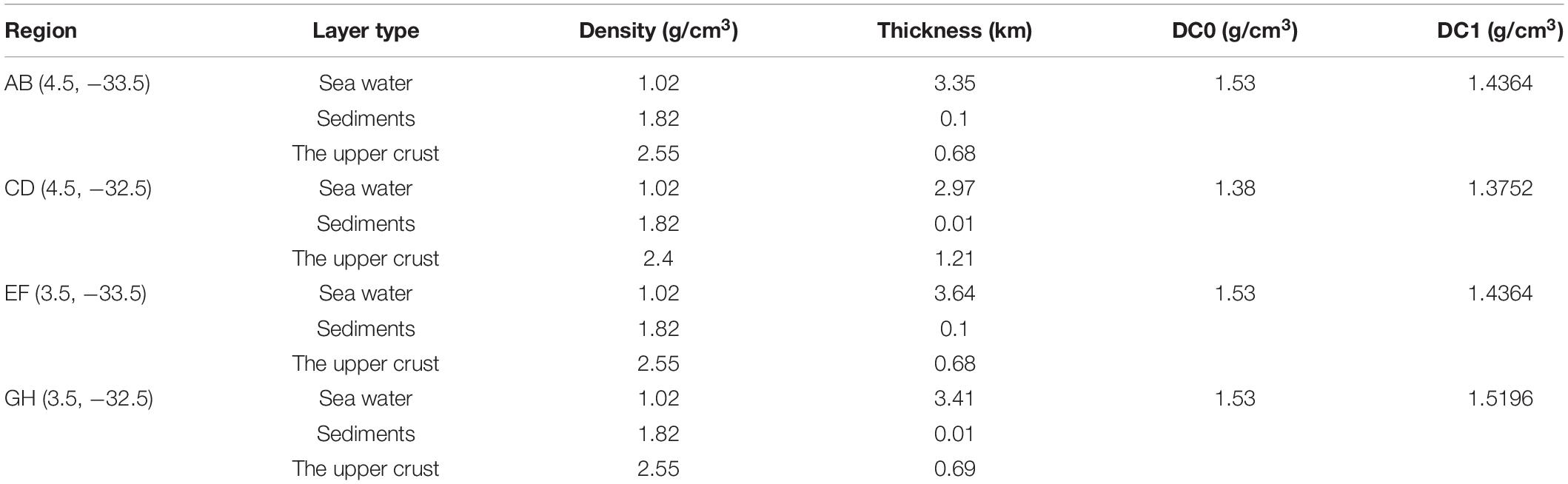
Table 1. Density contrasts from CRUST1.0.

It needs to be noted that the effects of sediments are not considered in the results of $\mathrm{\Delta }{\overline{\mathrm{\rho }}}_0$, but the results derived by the TLS contain the whole signals, including sediments. Hence, it is not accurate to ignore the sediments in the calculation of density contrasts using CRUST1.0 information, especially when the thickness of the sediments is large. In addition, the thickness of the sediments and the upper crust would also lead to the differences with TLS. In order to solve these issues, new density contrasts are derived as follows,

$$\mathrm{\Delta }\overline{\mathrm{\rho }}=\frac{{\mathrm{\rho }}_{sed}{H}_{sed}+{\mathrm{\rho }}_{c1}{H}_{c1}}{H_{sed}+H_{c1}}-{\mathrm{\rho }}_w(19)$$

in which, ρ_sed, ρ_c1 are respectively, the densities of the sediment layer and the upper crust; H_sed,H_c1 are the thicknesses of the sediment layer and the upper crust respectively; ρ_w is the density of the sea water. The newly derived results for each region are also given in Table 1.

Results and Analysis

Initial Results From TLS

Figure 3 shows the fitting results of TLS for each region, in which the x- and y-axis denote $(H-{\widehat{h}}_i)$ and $\mathrm{\Delta }{\widehat{g}}_i$ respectively. Please note, because the resolution of shipborne depths is much higher than DTU13, the shipborne depths are interpolated to the gird points of DTU13 before the TLS processing in order to make the two datasets have consistent resolution. It is found that the gravity anomalies show linear positive correlations with water depths (i.e.,$H-{\widehat{h}}_i$) in each subregion. For example, the larger the water depth, the larger the gravity anomaly. However, the slopes and intercepts of the fitting lines in each region are not the same. It can be inferred that this is caused by the complexity of the seabed geological structures.

FIGURE 3

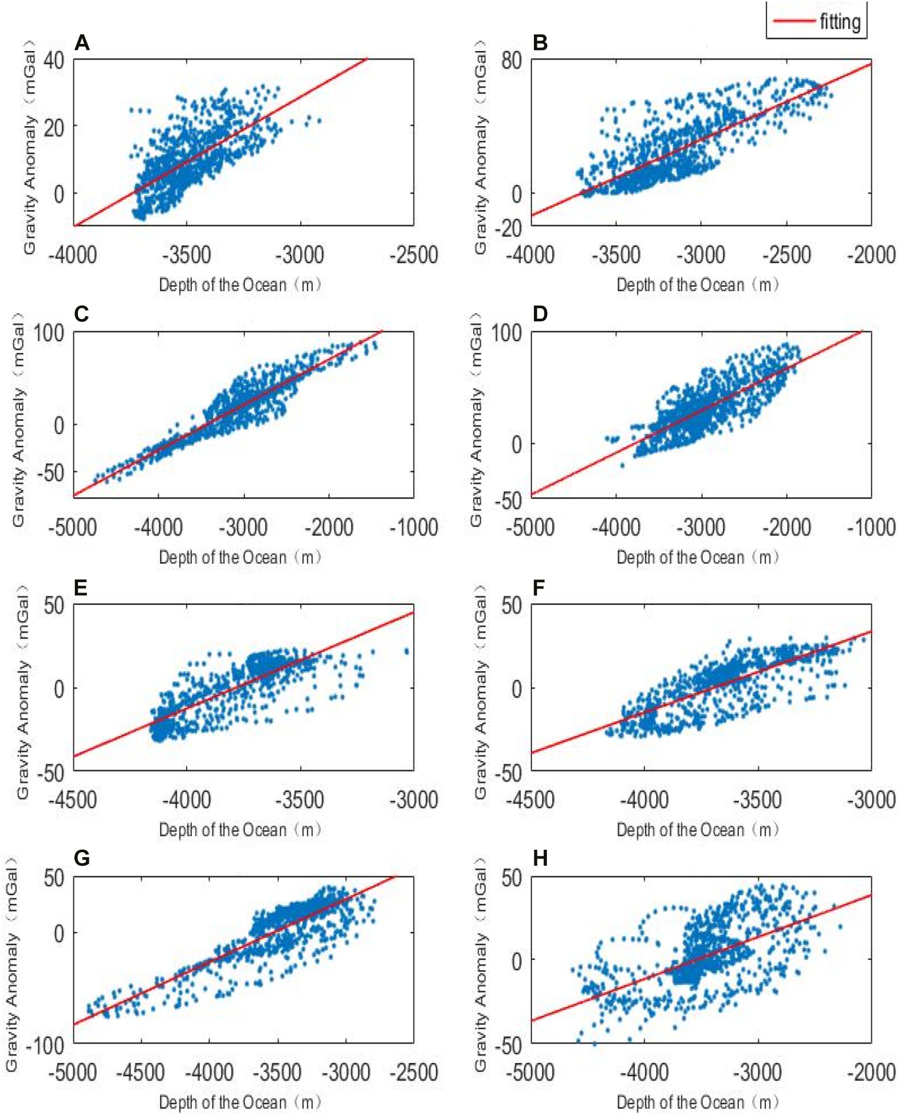
Figure 3. Lines of fit for each region. (A–H) represent the related regions defined in Figure 1.

The derived density results are shown in Table 2. It is found that the density contrasts of area A-H are in the range of 0.599–1.173 g/cm³, and the density contrasts are different due to the unique geological structure in each region. According to the SDUW, the fitting error in area A is the best, and that in area H is the worst. The accuracy of the whole area is between 6.124 and 14.493 mGal, among which the accuracy of area D and G is the closest, which indicates that the submarine geological structures in these two areas are similar. The SDUW of areas A and B have the largest difference in the adjacent areas, which may be caused by the large differences in the complicated seafloor geological structures between the two areas.

TABLE 2

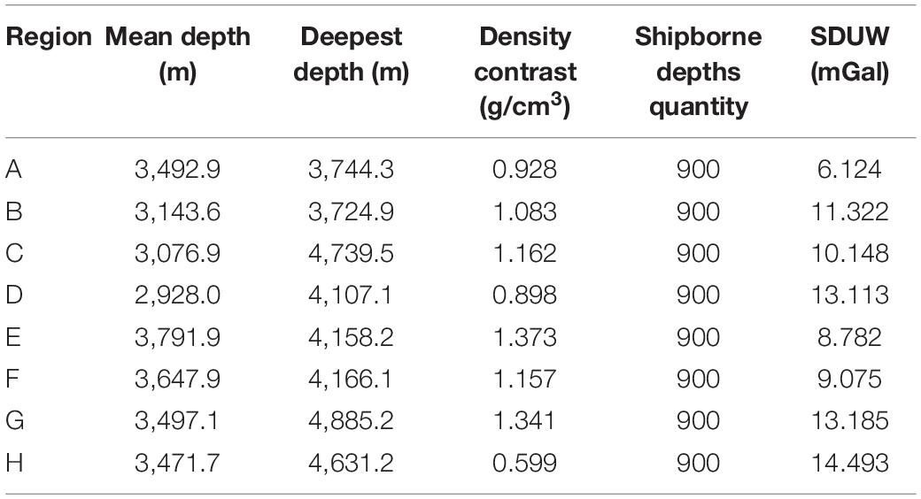
Table 2. Density results derived from TLS.

Compared to Table 1, the results from TLS are quite different from $\mathrm{\Delta }{\overline{\mathrm{\rho }}}_0$ and $\mathrm{\Delta }{\overline{\mathrm{\rho }}}_1$. Mean values of the whole study area are given in Table 3. It can be seen from the above table that the density contrasts obtained by CRUST1.0 model are much larger than that obtained by total least squares algorithm. The density contrast obtained by the weighted average method is closer to the result of TLS than that obtained by CRUST1.0 initial results, i.e., $\mathrm{\Delta }{\overline{\mathrm{\rho }}}_0$. Even so, the difference between the result of weighted average method and that obtained by total least squares is −0.374 g/cm³. If the values from CRUST1.0 are true values, the relative error exceed 25%. This indicates that the derived results are not very reliable. This conclusion is consistent with the fact that the density contrast derived in the GGM for bathymetry usually has no physical meaning (Annan and Wan, 2020).

TABLE 3

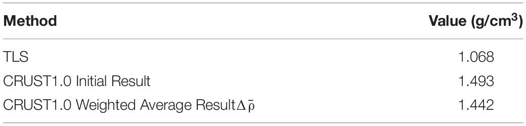
Table 3. Density contrast for the whole study area.

However, it should be noticed that the marine gravity anomalies are correlated with the information of the seafloor topography, including its depth and density contrast. In theory, if the density is known, the depths can be derived; if depths are known, the density can be derived. The possible reason why the large differences exist between the derived results with CRUST1.0 is that gravity anomalies have high correlations with seafloor topography only in a limited wave bandwidth (Marks and Smith, 2012; Wan et al., 2019). Although this issue has been considered in the derivation of bathymetry using GGM by modeling and removing the long wavelength gravity anomaly, the errors of the modeling would certainly cause some errors in the derivation of density contrast. In order to solve this issue, a filtering processing was added both to the gravity anomalies and shipborne depths and the new results are obtained in the next section.

New Results

Filtering Processing

The pass bands are designed by referring to studies about bathymetry, such as Smith and Sandwell (1994); Marks and Smith (2012). The sensitive band for bathymetry inversion is usually in the range of 20 ∼ 200 km (Hwang, 1999; Marks and Smith, 2012). This is also true for the density contrast inversion, because the mathematical function relationship is same as that used in bathymetry inversion, i.e., Equation 1. In order to reduce the effect from the non-sensitive bands, we decrease the band width which is usually used for bathymetry inversion and two pass bands are experimented, i.e., (30–100) km and (50–100) km.

As to why 100 km is selected as the maximum cutoff wavelength of the filtering pass-band, it is because the size of the study region is 1° × 2°; and thus, it is difficult to present signals with wavelength larger than 100 km due to the limited size, at least in the latitude direction. It is also because the spatial resolution of CRUST1.0 is 1° × 1°, corresponding to approximately 100 km × 100 km in spatial domain. As for the minimum cutoff wavelength of the pass-band, 30 and 50 km are defined as examples. Although, in bathymetry inversion, the minimum cutoff wavelengths of the pass-band are usually lower than 30 km, such as 20 or 15 km (Abulaitijiang et al., 2019), this study enlarges the minimum cut-off wavelength of the pass-band in order to ensure a higher correlation between the filtered shipborne depths and gravity anomalies. It is difficult to obtain the most sensitive band from gravity anomaly to bathymetry (Wan et al., 2019) like in gravity gradient to bathymetry. It is also true between the gravity anomaly and density contrast, since the mathematical relationship are same in bathymetry and density contrast inversions.

As an example, the filter for pass-band (30–100) km as well as the filtered data are shown in Figures 4, 5 respectively. In Figure 4, the red dotted lines denote the cutoff wavelength, i.e., 30 and 100 km. Compared to Figure 2, the similarity between gravity anomaly and ship-depths shown in Figure 5 is definitely much stronger. This indicates the correlations between the two data sets are higher than that of the data shown in Figure 2. This point is proved further by Table 4, which shows the correlations between the ship-depths and gravity anomalies in each sub-region. Obviously, the correlations are improved largely by the filtering processing. Especially for the region H, the improvements in the correlations arrive at 35% compared to the initial correlations.

TABLE 4

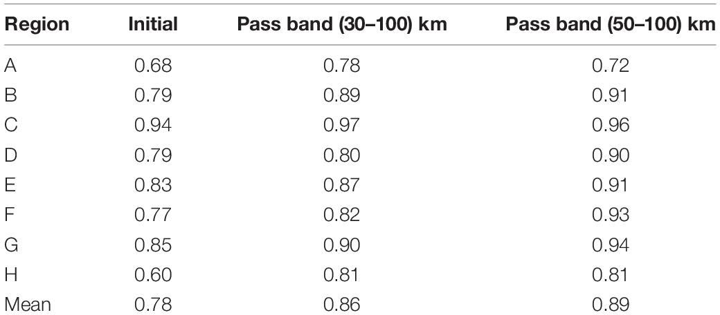
Table 4. Correlations between shipborne depths and gravity anomalies in each region.

FIGURE 4

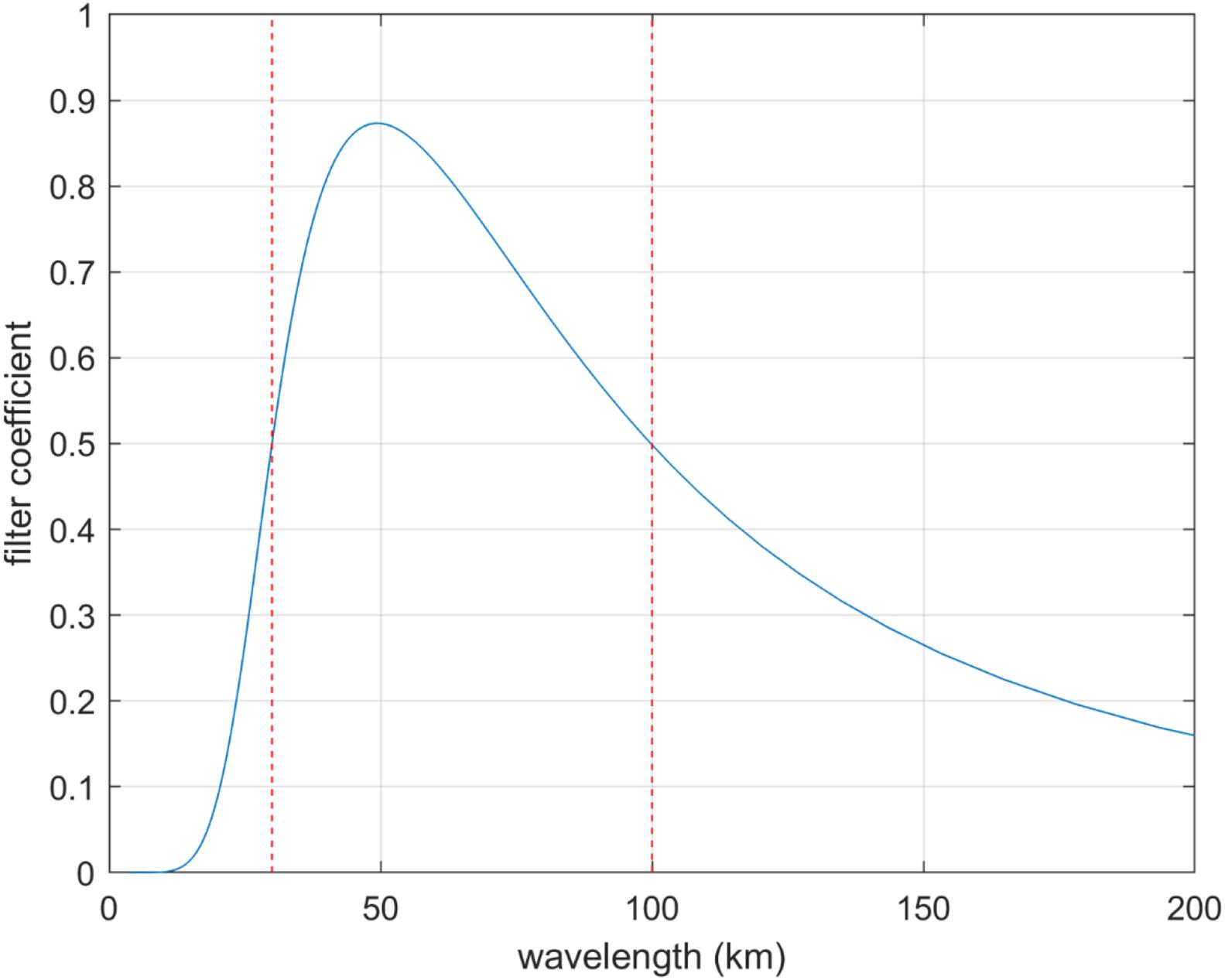
Figure 4. The filter with pass-band (30–100) km.

FIGURE 5

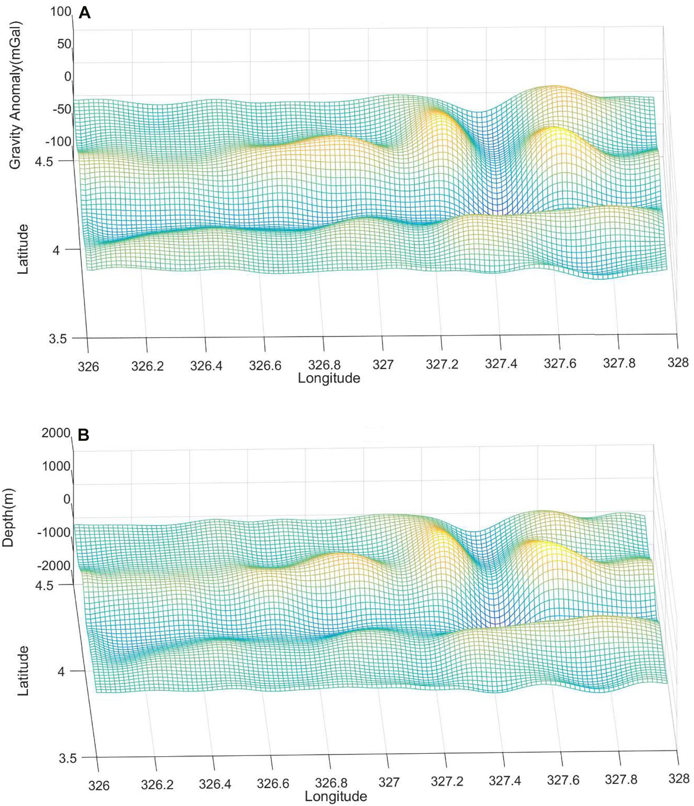
Figure 5. The filtered gravity anomaly (A) and shipborne depths (B).

New Results

By band-pass filtering gravity anomalies and shipborne depths data, density contrasts are again derived using TLS and shown in Table 5. And the comparisons with weighted mean values of CRUST1.0 are given in Table 6. We named the pass-band (30–100) km as pass-band1 and the pass-band (50–100) km as pass-band2 in this study.

TABLE 5

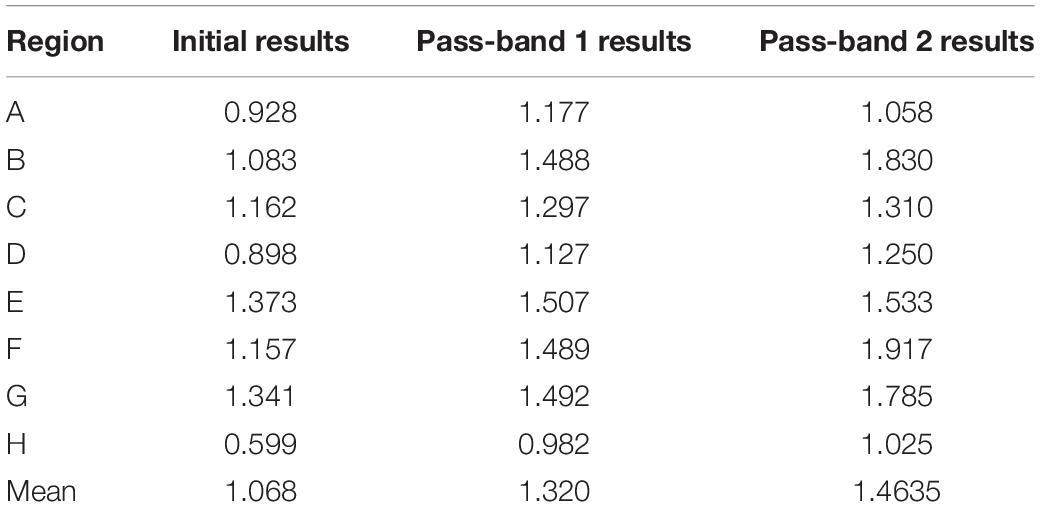
Table 5. Density contrasts derived with TLS by adding a filtering processing (unit: g/cm³).

TABLE 6

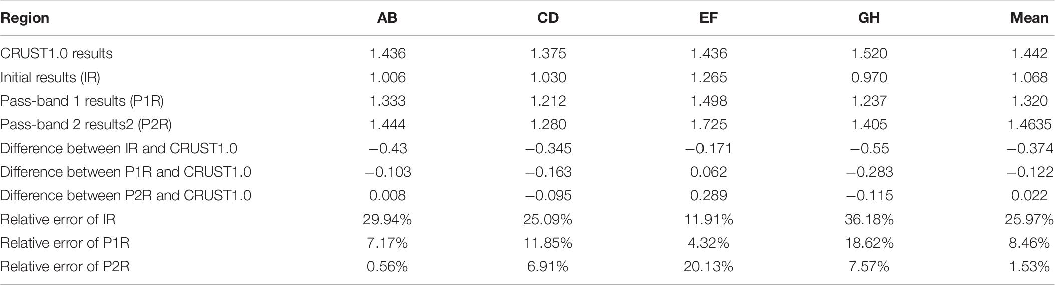
Table 6. Comparisons with derived results and CRUST1.0 (unit: g/cm³).

Definitely, the new results are much closer to CRUST1.0 than the initial results and the differences are reduced by more than 60% in the total area. The magnitude of the differences between the new results and CRUST1.0 are smaller than 0.13 g/cm³ and 0.03 g/cm³ for the two pass-bands in terms of mean value of the whole area. If the CRSUT1.0’s value is the true value, i.e., 1.442 g/cm³, the relative errors of the two pass-bands are 8.46% and 1.53%, respectively. In general, in the whole area, the pass-band2, i.e., (50–100) km, yields closer results to CRUST1.0. However, in Region EF, the difference becomes larger. This may be due to the fact that the spatial resolution of CRUST1.0 is not enough to present the density contrast variation in local regions with size smaller than 1° × 1°. This would be investigated further in the future.

Please note, no information of CRUST1.0 is used in the inversion. Since the results are now close to CRUST1.0, it proves that marine gravity anomalies and shipborne depths can be used to derive seafloor density contrasts with a high accuracy. It also proves that the proposed method is effective. It should be emphasized that the spatial resolution of CRUST1.0 is only at 1.0 degree but it is not the case for gravity anomaly and even the shipborne depths. Hence, it is fully possible to derive the density contrast information all over the ocean with a much higher spatial resolution than CRUST1.0, because highly accurate gravity anomalies can be provided by several altimetry missions and a very large amount of shipborne depth observations have been collected by NOAA. The global inversion would be conducted in the future study.

Discussion

In order to show the influence of the bathymetry undulation on density contrast inversion, the mean, deepest, and standard deviation (Std) values of the depths in each subregion are presented in Table 7. Comparing Tables 6, 7, it is found that the deeper the water depths, the lower the inversion accuracy if the region EF is not considered. For example, in the initial shipborne depths, the absolute values of the mean and the deepest depths in GH region are all larger than regions AB and CD. Correspondingly, the inversion accuracy in region GH is much lower than those of regions AB and CD. Even after filtering, the maximum depth in region GH is still larger than those of regions AB and CD; and thus, the accuracy in region GH is still the lowest among the three regions. This phenomenon may be due to the fact: the deeper the water depth, the lower the gravity anomaly signals at the sea surface generated by density body of the seafloor. Since the gravity anomaly accuracies are almost same in the study subregions, the signal to noise ratio (SNR) must be different with different water depths. In general, the SNR of GH is lower than that of other regions. Hence, the density contrast inversion accuracy in the deep ocean area would be poorer than other areas. Because of this, in order to obtain the same inversion accuracy, the gravity anomaly should have a higher accuracy in the deep ocean regions than areas with shallower water depths.

TABLE 7

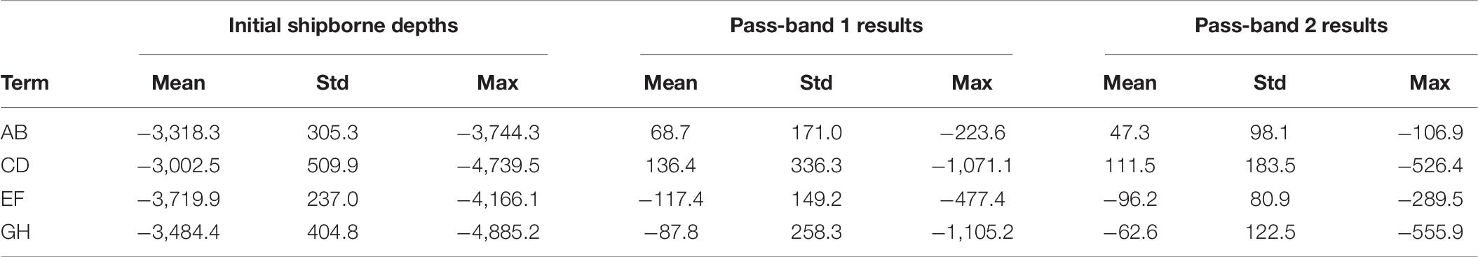
Table 7. Depth statistics (unit:m).

It should be noted that the inversion results of region EF are not consistent with the above phenomenon. This may be caused by the limited spatial resolution of CRUST1.0, which is not enough to present the regional information. In order to check accuracy of CRUST1.0, we compare the sea water depths given by CRUST1.0 with shipborne depths used in this study. The statistics is given in Table 8, in which the differences between shipborne depths and CRUST1.0 are given and the relative error represents the ratio of the difference to shipborne depth value. According to Table 8, mean water depths provided by CRUST1.0 are very close to the shipborne depths and the mean differences are smaller than 100 m. If shipborne depths are the true values, the accuracy of CRUST1.0 is poorest in Region EF. This means it is better to use other data to evaluate the inversion accuracy in Region EF. Unfortunately, this study currently could not obtain the related available data; and hence, the evaluation would be conducted in near future if other highly accurate seafloor density datasets become available.

TABLE 8

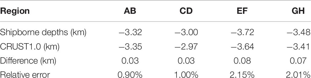
Table 8. Mean water depth statistics.

Conclusion

This study presented a study for seafloor density contrast inversion using gravity anomalies and shipborne depth datasets. The inversion was achieved by a total least squares algorithm, which considers both noises from gravity anomalies and shipborne depths. The results show that if gravity anomaly and shipborne depths are used directly, the derived density contrasts contain large errors, which may be caused by the modeling error of the long wavelength part of gravity anomalies. Hence, a band pass filtering technique was proposed to resolve this issue and the final results show an obvious accuracy improvement of the derived density contrast, and thus verified the effectiveness of the method.

As for the sensitive band, in general it is the band of 20 ∼ 200 km. However, in density contrast inversion, it would be better to only use signals in a part of the sensitive band if it is defined as where the correlation is larger than 0.5, because the high correlation between the gravity data and shipborne depths would help improve the inversion accuracy. Therefore, we suggest that the determination of the pass-band of the filter is done by a correlation analysis between the gravity anomaly and shipborne depths, and the sensitive band can be defined as the bands with correlations larger than 0.85 or even higher between the two data sets to ensure high correlation in the pass-band.

Since various altimetry satellite missions (Hwang et al., 2002; Sandwell et al., 2014a; Wan et al., 2019; Zhu et al., 2020) have provided enough observations to derive highly accurate and dense marine gravity products and a large amount of shipborne depths data have been collected by NOAA, high accuracy and resolution of density contrasts can be derived for major areas of the global ocean by the proposed method in this study. In addition, gravity gradient products derived by some institutes (Hwang and Chang, 2014; Sandwell et al., 2014a) may also contribute a lot in the inversion.

Data Availability Statement

Publicly available datasets were analyzed in this study. This data can be found here: The gravity data can be downloaded from the DTU space center website: https://www.space.dtu.dk/english/Research/Scientific_data_and_models/Global_Marine_Gravity_Field. CRUST1.0 is available from the website: https://igppweb.ucsd.edu/~gabi/crust1.html. The shipborne depths used in this study are available on the request to the corresponding author.

Author Contributions

XW, WH, JR, and BL: conceptualization and investigation. XW, WH, WM, and RA: data curation and methodology. XW: funding. XW, JR, and RA: writing—original draft. XW, WH, JR, WM, RA, and BL: writing—review and editing. All authors read and approved the final manuscript.

Funding

This work was funded by the National Natural Science Foundation of China (Nos. 41674026 and 42074017); Fundamental Research Funds for the Central Universities (No. 2652018027); Open Research Fund of Qian Xuesen Laboratory of Space Technology, CAST (No.GZZKFJJ2020006); and China Geological Survey (No. 20191006).

Conflict of Interest

The authors declare that the research was conducted in the absence of any commercial or financial relationships that could be construed as a potential conflict of interest.

Acknowledgments

We would like to thank First Institute of Oceanography, Ministry of Nature Resources for providing ship sounding data and DTU for providing gravity anomaly data and Institute of Geophysics and Planetary Physics for providing CRUST1.0 data.

Footnotes

1. ^ https://ftp.space.dtu.dk/pub/DTU13/1_MIN/

References

Abulaitijiang, A., Andersen, O. B., and Sandwell, D. (2019). Improved Arctic ocean bathymetry derived from DTU17 gravity model. Earth Space Sci. 6, 1336–1347. doi: 10.1029/2018EA000502

CrossRef Full Text | Google Scholar

Andersen, O. B. (2010). “The DTU10 gravity field and mean sea surface,” in Proceedings of the Second International Symposium of the Gravity Field of the Earth (IGFS2) (Fairbanks, AK).

Google Scholar

Andersen, O. B., Knudsen, P., and Berry, P. (2010). The DNSC08GRA global marine gravity field from double retracked satellite altimetry. J. Geod. 84, 191–199. doi: 10.1007/s00190-009-0355-9

CrossRef Full Text | Google Scholar

Andersen, O. B., Knudsen, P., Kenyon, S., and Holmes, S. (2014). “Global and Arctic marine gravity field from recent satellite altimetry (DTU13),” in Proceedings 76th EAGE Conference and Exhibition 2014 (Amsterdam), doi: 10.3997/2214-4609.20140897

PubMed Abstract | CrossRef Full Text | Google Scholar

Annan, R. F., and Wan, X. (2020). Mapping seafloor topography of Gulf of Guinea using an adaptive meshed gravity-geologic method. Arab. J. Geosci. 13:301. doi: 10.1007/s12517-020-05297-8

CrossRef Full Text | Google Scholar

Bassin, C. (2000). The current limits of resolution for surface wave tomography in North America. Eos Trans. AGU 81:F897.

Google Scholar

Felix, W., Regina, L., Edi, K., and Ansorge, J. (2002). High-resolution teleseismic tomography of upper-mantle structure using an a priori three-dimensional crustal model. Geophys. J. Int. 150, 403–414. doi: 10.1046/j.1365-246X.2002.01690.x

CrossRef Full Text | Google Scholar

Golub, G. H., and van Loan, C. F. (1980). An analysis of the total least squares problem. SIAM J. Numer. Anal. 17, 883–893. doi: 10.1137/0717073

CrossRef Full Text | Google Scholar

Hsiao, Y., Kim, J., Kim, K., Lee, B. Y., and Hwang, C. (2011). Bathymetry estimation using the gravity-geologic method: an investigation of density contrast predicted by downward continuation method. Terr. Atmos. Ocean Sci. 21, 347–358. doi: 10.3319/TAO.2010.10.13.01(Oc)

CrossRef Full Text | Google Scholar

Hu, M., Li, J., Li, H., Shen, C. Y., and Xing, L. (2015). Predicting global seafloor topography using Multi-source data. Mar. Geod. 37, 176–189. doi: 10.1080/01490419.2014.934415

CrossRef Full Text | Google Scholar

Hwang, C. (1999). A bathymetric model for the south China Sea from altimetry and depth data. Mar. Geod. 22, 37–51. doi: 10.1080/014904199273597

CrossRef Full Text | Google Scholar

Hwang, C., and Chang, E. (2014). Seafloor secrets revealed. Science 346, 32–33. doi: 10.1126/science.1260459

PubMed Abstract | CrossRef Full Text | Google Scholar

Hwang, C., Hsu, H. Y., and Jang, R. J. (2002). Global mean sea surface and marine gravity anomaly from multi-satellite altimetry: applications of deflection-geoid and inverse Vening Meinesz formulae. J. Geod. 76, 407–418. doi: 10.1007/s00190-002-0265-6

CrossRef Full Text | Google Scholar

Ibrahim, A., and Hinze, W. (1972). Mapping buried bedrock topography with gravity. Ground Water 10, 18–23. doi: 10.1111/j.1745-6584.1972.tb02921.x

CrossRef Full Text | Google Scholar

Jiang, Y., Zhang, Y., Wang, S., Jiao, J., and Huai, Y. (2015). Inversion of Moho depth in western China considering gravity correction of deposition layer. J. Seismol. Res. 38, 257–261.

Google Scholar

Kim, J., Frese, R., Lee, B., Roman, D., and Doh, S. (2011). Altimetry-derived gravity predictions of bathymetry by gravity-geologic method. Pure Appl. Geophys. 168, 815–826. doi: 10.1007/s00024-010-0170-5

CrossRef Full Text | Google Scholar

Laske, G., Masters, G., Ma, Z., and Pasyanos, M. (2013). Update on CRUST1. 0–A 1-degree global model of earth’s crust. Geophys. Res. Abstr. 15:20132658abstrEGU.

Google Scholar

Marks, K. M., and Smith, W. H. F. (2012). Radially symmetric coherence between satellite gravity and multibeam bathymetry grids. Mar. Geophys. Res. 33, 223–227. doi: 10.1007/s11001-012-9157-1

CrossRef Full Text | Google Scholar

Mooney, W. D., Laske, G., and Masters, T. G. (1998). CRUST 5.1: a global crustal model at 5° x 5°. J. Geophys. Res. Solid Earth 103, 727–747. doi: 10.1029/97JB02122

CrossRef Full Text | Google Scholar

Nagendra, R., Prasad, P. V. S., and Bhimasankaram, V. L. S. (1996). Forward and inverse computer modeling of a gravity field resulting from a density interface using Parker-Oldenburg method. Comput. Geosci. 22, 227–237. doi: 10.1016/0098-3004(95)00075-5

CrossRef Full Text | Google Scholar

Nataf, H. C., and Ricard, Y. (1996). 3SMAC: an a priori tomographic model of the upper mantle based on geophysical modeling. Phys. Earth Planet. Inter. 95, 101–122. doi: 10.1016/0031-9201(95)03105-7

CrossRef Full Text | Google Scholar

Ouyang, M., Sun, A., and Zhai, Z. (2014). Predicting bathymetry in south china sea using the gravity geologic method. Chin. J. Geophys. 57, 2756–2765. doi: 10.6038/cjg20140903

CrossRef Full Text | Google Scholar

Parker, R. L. (1972). The rapid calculation of potential anomalies. Geophys. J. R. Astron. Soc. 31, 447–455. doi: 10.1111/j.1365-246X.1973.tb06513.x

CrossRef Full Text | Google Scholar

Sandwell, D., Carcla, E., and Smith, W. (2014b). Recent Improvements in Arctic and Antarctic Marine Gravity: Unique Contributions from CryoSat-2, Jason-1, Envisat, Geosat and ERS-1/2, Amercial General Union (AGU). (accessed November 29, 2014).

Google Scholar

Sandwell, D., Muller, R., Smith, W., Garcia, E., and Francis, R. (2014a). New global marine gravity model from CryoSat-2 and Jason-1 reveals buried tectonic structure. Science 346, 65–67. doi: 10.1126/science.1258213

PubMed Abstract | CrossRef Full Text | Google Scholar

Smith, W. H. F., and Sandwell, D. T. (1994). Bathymetric prediction from dense satellite altimetry and sparse shipboard bathymetry. J. Geophys. Res. Solid Earth 99, 21803–21824. doi: 10.1029/94JB00988

CrossRef Full Text | Google Scholar

Soller, D. R., Ray, D., and Brown, R. D. (1982). A new global crustal thickness map. Tectonics 1, 125–149. doi: 10.1029/TC001i002p00125

CrossRef Full Text | Google Scholar

Wan, X., Ran, J., and Jin, S. (2019). Sensitivity analysis of gravity anomalies and vertical gravity gradient data for bathymetry inversion. Mar. Geophys. Res. 40, 87–96. doi: 10.1007/s11001-018-9361-8

CrossRef Full Text | Google Scholar

Xiang, X., Wan, X., Zhang, R., Li, Y., Sui, X., and Wang, W. (2017). Bathymetry inversion with Gravity-Geologic Method: a study of long-wavelength gravity modeling based on adaptive mesh. Mar. Geod. 40, 329–340. doi: 10.1080/01490419.2017.1335257

CrossRef Full Text | Google Scholar

Xu, P. L., Liu, J., and Shi, C. (2012). Total least squares adjustment in partial errors-in-variables models: algorithm and statistical analysis. J. Geod. 86, 661–675. doi: 10.1007/s00190-012-0552-9

CrossRef Full Text | Google Scholar

Zhu, C., Guo, J., Gao, J., Liu, X., Hwang, C., Yu, S., et al. (2020). Marine gravity determined from multi-satellite GM/ERM altimeter data over the South China Sea: SCSGA V1.0. J. Geod. 94:50. doi: 10.1007/s00190-020-01378-4

CrossRef Full Text | Google Scholar