3D Printing the World: Developing Geophysical Teaching Materials and Outreach Packages

1. Introduction

In global geophysics, we are concerned with understanding various properties of the subsurface and the Earth's interior. Spatial variations in these properties are generally represented as 2D coloured or contoured maps and cross sections. Conveying the 3D nature of many of these structures can be difficult, but is crucial to understanding the processes occurring within the Earth. 2D global maps often fail to convey the area, shape, distance, and continuity of features, particularly at the poles where global map projections are usually most distorted. For this reason, comparing features between low and high latitudes can be difficult. Equally, typical colour bars can be unintentionally biasing or inadvertently inaccessible to the colour-blind (e.g., Crameri et al., 2020; Stauffer and Zeileis, 2020), and even well chosen colour bars do not convey accurately the shape of many features. Many of these limitations are overcome by 3D visualisation tools such as Paraview (www.paraview.org) or Gplates (Müller et al., 2018), but these require skill to operate and are not suited to all settings such as schools, poster presentations and outdoor events. 3D-printed objects, such as the globes presented here, complement these traditional methods by presenting tactile, engaging, undistorted and inherently 3D representations of geophysical fields, which are beneficial both in structured education and public engagement settings.

3D printing refers to an expanding set of additive manufacturing techniques for creating physical objects from digital designs. While many different technologies exist, the last 5 years has seen a dramatic increase in the availability of cheap desktop 3D printers that use a technique known as fused filament fabrication (FFF). Functioning by building up objects layer by layer from extruded, sustainable bio-plastic, capable FFF printers are now available for as little as $200 thanks to open source designs based on off-the-shelf components. With the reduction in cost and increase in availability, 3D printers have become more accessible and are increasingly common within educational institutions. As a result, intricate, bespoke 3D objects such as our globes, which would be cost-prohibitive to manufacture in low production volumes by other methods such as injection moulding, are cheap and easy to produce (Berman, 2012). They can also be distributed digitally for free and incorporated into lesson plans and public engagement events wherever and whenever they are needed.

Ford and Minshall (2019) identified six usage categories for 3D printing in education, of which our globes support three: to produce artefacts that aid learning, to create assistive technologies and to support outreach activities.

Firstly, our globes aid learning by complementing traditional 2D representations and help students to engage through their novelty. 3D printing makes communication in teaching more effective, making use of intuition and touch (Hasiuk et al., 2017). This particularly helps students who have difficulty understanding 3D concepts and helps them to acquire 3D skills (Hasiuk and Harding, 2016). Having physical, tangible objects such as our globes aids in setting up an active learning environment, a practice that is backed up by the review of Prince (2004) and the good teaching practices of Chickering and Gamson (1987). The use of physical objects in interactive lessons also helps the attention span of students and improves the recall of material (Stuart and Rutherford, 1978).

Secondly, our globes make geophysical data accessible to the visually impaired—something not achievable through text based descriptions. This is important in seeking to address the under-representation of the visually impaired community in university education and to encourage young people with vision impairments to study STEM subjects. Efforts to use 3D printing and associated techniques to engage the visually impaired community have already proven successful, particularly in astronomy, for example through the Tactile Universe project (Bonne et al., 2018)—see also the review by Arcand et al. (2020). Several initiatives in geology have also embraced 3D printing, particularly in palaeontology and at local and regional scales (e.g., Hasiuk et al., 2017; Ishutov et al., 2018). However, on a global scale and in global geophysics, we believe our globes are novel and can make an important contribution.

Thirdly, our globes have already been used in several public engagement events, where the public have been encouraged to engage with our science in ways that would not have been possible with traditional 2D maps. Whilst the Covid-19 pandemic has prevented us from collecting formal feedback, our subjective experience is that the globes are excellent both at attracting an audience who wish to see what they are and in helping to convey complex concepts. The tactile objects and the novelty of the 3D printing technology tend to make people more curious, leading to an increase in interaction and interest in the geosciences (Hasiuk et al., 2017).

In this contribution, we focus on geophysical scalar fields, which are often unintuitive (e.g., the geoid), and/or abstract (such as seismic velocities deep within the Earth). We present a workflow for representing these fields as 3D-printable objects that can be explored in teaching settings and used for public engagement events (Figure 1). We discuss examples of specific 3D-printed globes that we have developed, covering both the specifics of the models and how they can be used for education and public engagement. Our models range in complexity from simple topographic models of planetary bodies to layered representations of complex geophysical fields. Finally, we discuss the limitations of our workflow and provide suggestions for alternative materials that can be used.

FIGURE 1

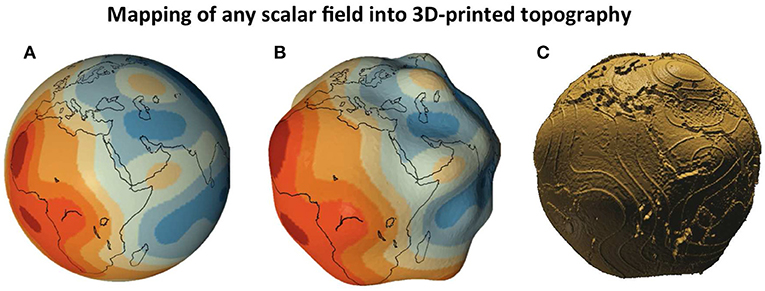
Figure 1. Illustration of how any scalar field can be represented as a 3D-printable model. This example shows how seismic velocity variations at 2,850 km depth are transformed to 3D topography. In this example, low seismic velocities (red in A,B) are represented by elevated topography. The final model (C) still conveys the information without using colour, using embossed contours to add interpretation and continental outlines for spatial context.

2. Methodology

3D models are created by a 3-step process: (1) create greyscale height map images from global gridded data, (2) composite these height map images into a single image and (3) apply this to the surface of a sphere to produce 3D models for printing. An example of this workflow is presented in Figure 2 and a detailed step-by-step guide is provided in the Supplementary Material. The key components of our workflow are:

• The Generic Mapping Tools (GMT) (Wessel et al., 2013), used for gridding and processing data and creating height maps

• Python code and standard libraries (https://www.python.org/), used for compositing height maps

• Blender (https://www.blender.org/), used to create and manipulate 3D models

• Autodesk Meshmixer (http://www.meshmixer.com/), optionally, to optimise models for 3D printing

• PrusaSlicer (https://www.prusa3d.com/prusaslicer/), used to slice 3D models into printable “gcode” files

• A desktop FFF 3D printer such as the Prusa i3 mk3 (https://github.com/prusa3d/Original-Prusa-i3), the design for which is open source and has facilitated the boom in affordable desktop 3D printing

We will now describe these steps and components in more detail.

FIGURE 2

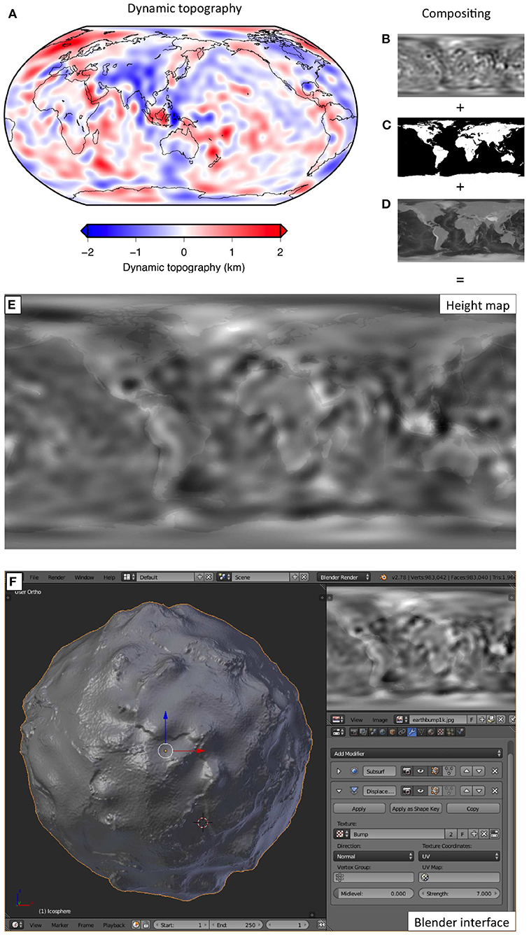
Figure 2. Overview of the key steps of our 3D modelling workflow, using dynamic topography as an example. (A) Traditional 2D map with polar colour bar. Individual greyscale height maps (B–D) are combined to give a single composite height map (E). The dynamic topography field (B) provides the long wavelength component, continental outlines (C) provide spatial reference, and ETOPO1 surface topography (D) provides geological features such as sea mounts and trenches. The composite height map (E) is applied to the surface of a sphere in Blender (F) producing a final 3D globe. Input images were generated using the Generic Mapping Tools (Wessel et al., 2013) and composited using Python. For more details see the Supplementary Material.

2.1. Height Map Creation

The Blender workflow outlined below (and in detail in the Supplementary Material) requires “height maps,” also known as displacement maps or bump maps. These maps are simple greyscale images in a Cartesian or Plat Carée projection that cover the full global range of longitude and latitude. The lightness of the image corresponds to the topography on the final 3D model, such that white is the maximum positive displacement (bumps), mid grey is neutral and black is the maximum negative displacement (depressions).

Open source and academic datasets such as planetary topography (e.g., NOAA, 2009; Smith et al., 2010), coastline information (GSHHG, Wessel and Smith, 1996) and more niche geophysical scalar fields such as the geoid (Foerste et al., 2014), dynamic topography (Hoggard et al., 2016) and seismic tomography models (e.g., SP12RTS, Koelemeijer et al., 2016) are provided in various formats. The Global Mapping Tools (Wessel et al., 2013) are used to turn these datasets into greyscale images in any lossless 8-bit format, such as PNG or TIFF. 8-bit images are used for compatibility reasons—this means that height maps are quantised to 256 evenly spaced levels, which can become visible on high displacement or very long wavelength models. During the original workflow development, compatibility in Blender required 8-bit images, but this limitation may be removed in newer versions.

2.2. Height Map Compositing

Geographic context is critical for understanding the meaning of geophysical parameters. For example, the location of a mantle plume beneath Iceland is demonstrated by the underlying low seismic velocity anomaly. In order to provide this context we composite our geophysical height maps with topography and coastline height maps (Wessel and Smith, 1996; NOAA, 2009) by adding them together and re-scaling to an 8-bit integer format (Figures 2B–E). Relative scaling factors are determined aesthetically. However, it is important to take note of the scaling factor of the geophysical height map for the calculation of vertical exaggeration factors. The compositing and relative scaling is accomplished using Python3 in a Jupyter notebook, available in the Supplementary Material, which relies on the numpy, PIL, and imageio libraries.

2.3. 3D Modelling

3D models are created in Blender by applying a displacement modifier to a simple sphere, the detailed workflow for which is provided in the Supplementary Material along with a sample project file (see also Figure 2F). The technique of UV mapping relates the coordinates of the pixels in the height map to the position on a sphere. Subdivision (procedurally increasing the number of vertices in the model) prior to UV mapping gives substantially better results at the poles. The displacement modifier accepts two variables in addition to the height map image, corresponding to a magnitude of topography (expressed in the units of the Blender project) and a midpoint to define the neutral level. The models thus created can be easily exported for 3D printing as triangulated 3D meshes of standard formats, such as STL or OBJ files.

Prior to printing, the resulting 3D models are hollowed and cut into two hemispheres along the equator. The hollowing reduces the amount of time and material required for printing, while separating into hemispheres allows both for a flat surface that adheres to the print bed and gives the best results for print quality by minimising overhangs. This manipulation can be accomplished either in Blender or Autodesk Meshmixer, the latter of which is not open source and is only available for Microsoft Windows and macOS, but is nevertheless free to use. We chose to use Meshmixer because it is designed specifically for 3D printing and therefore contains specific tools for checking printability.

2.4. 3D Printing

Our models are easily and cheaply printed in 6–8 h on desktop Fused Filament Fabrication (FFF) printers, of which there are many hundreds to choose from and which cost as little as $200. Our models typically cost $2–$5 per print for a typical 8 cm diameter globe, which works well in a classroom environment or public engagement setting.

Slicing, the process by which 3D models are converted into 3D printer instructions, can be accomplished in many different open source software packages including PrusaSlicer and Ultimaker Cura. Whilst the specific settings required will depend on the printer model, the material being used, the software package and the choices of the user, we offer the following advice. Our models can be printed without support material, since the overhanging interior will not be visible in the final model when glued together, drastically reducing the amount of material used. PolyLactic Acid (PLA) bioplastic filament is an excellent choice of material, as it is cheap, non-toxic, low-shrinkage, high detail and does not derive from fossil fuels.

2.5. Advanced Models

In addition to the simple globes we develop using the described methodology, we have created more sophisticated models. Using Boolean operations in Blender it is possible to combine multiple 3D models to aid specific teaching plans. Examples of these include Earth topography globes that open to expose the outer core and inner core, explaining Earth's interior structure, and crustal thickness globes, which show the correspondence of high surface topography to deep crustal roots. Most of these advanced globes are held together by adding magnet holes in Meshmixer and embedding cheap neodymium magnets during the printing process, following the workflow of Telling (2019).

Our workflow can be used to represent any scalar field, whether this physically represents topography or not. In order to 3D print any scalar field, we linearly map the field in question to topographic variations, generally choosing the polarity by making a sensible interpretation of what the scalar field represents. Geographic context is provided by compositing this false topography with actual surface topography. For this reason, long-wavelength (>500 km) fields give better results as they can be easily distinguished from the actual surface topography. We use this approach to create our seismic tomography globes, nesting globes that show how the Earth's seismic velocity structure varies with depth (Figure 1). In this case, low seismic velocities are represented as topographic highs, thus reflecting the idea that these low velocities correspond to upwellings.

2.6. Model Sharing

A thriving online 3D printing community has developed and thus there are many free to use sharing platforms. We place all of our models in the public domain using the Thingiverse platform, making them available for free without restrictions on their use (see the Data Availability Statement for details). We have also endeavoured to ensure that our methodology is based on open source and free to use software, data and even hardware. This approach is intended to ensure that there is no unavoidable barrier to these tools or models being used for educational purposes.

3. Results: Examples of Use

In this section, we present examples of 3D-printed globes that we have developed. In each case, we discuss the context of the 3D-printed globe, the origin of the data used to build the 3D model and what topics can be explained using the 3D-printed globe. Some globes, like the planetary topography and seismic tomography ones, are discussed in more detail, as they have been used frequently. Our suggested discussion topics are mostly predicated on a public engagement setting, but they can easily be adapted to a classroom environment.

Our globes have so far only been displayed at a small number of predominantly public engagement events. Unfortunately, our intention to quantify their impact by use of questionnaires and statistics has been precluded by the cancellation of many events due to the coronavirus pandemic. Therefore, our assessment of the efficacy and impact of our models is necessarily subjective at the moment.

3.1. Planetary Topography

The surface of a planet reflects the dynamic processes that happen within its interior. On Earth, the surface is continually renewed due to the presence of plate tectonics, which demonstrates that we live on a dynamic planet. Models of planetary topography can thus be used to explain tectonic and other processes that shape the surface of a planet.

We have developed a set of 3D-printed globes of planetary topography (Figure 3). At the moment, we have chosen to include Earth, Mars, and the Moon, as together these three planetary bodies are sufficient to discuss a range of topics. Earth is full of tectonic features, reflecting the presence of plate tectonics, while the Moon is covered in craters of different sizes, indicating that it is primarily subject to external forces. Mars falls in between these two, as it shows evidence of tectonic features while also featuring craters on part of its surface. Their 3D-printed globes can thus be used to discuss the importance of tectonic processes on planetary topography, and to answer questions like: “How is planetary topography influenced by internal and external processes?” and “What we can learn from studying planetary topography?”

FIGURE 3

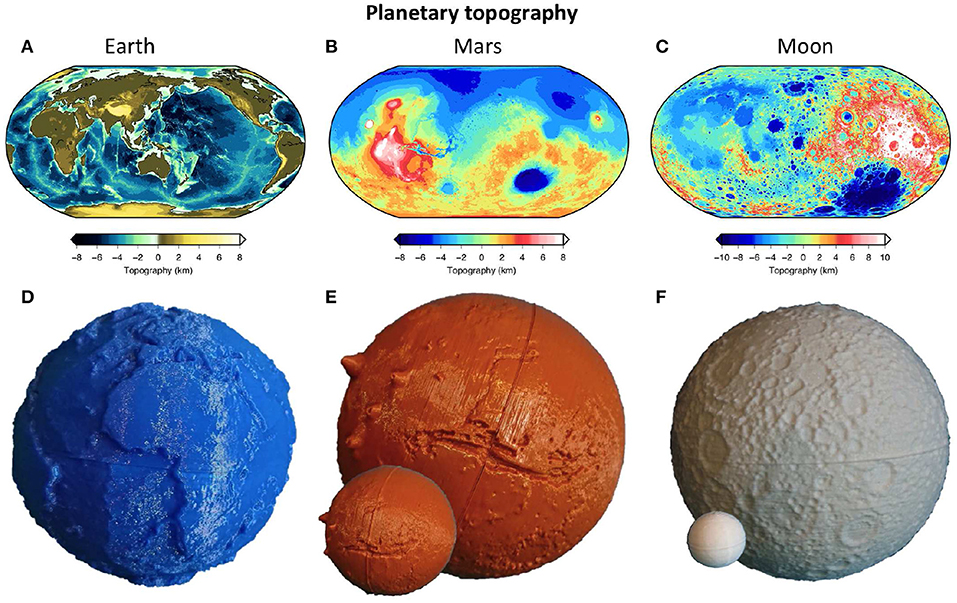
Figure 3. 2D maps and 3D-printed globes of the topography of different planetary bodies, including (A,D) Earth, (B,E) Mars, and (C,F) the Moon. This set of five globes is used to explain the concepts of plate tectonics for shaping the surface of a planet: Earth's surface is constantly reworked by plate tectonics, the Moon is covered in ancient craters and Mars shows tectonic features as well as impact craters. The three main globes are each approximately 8 cm in diameter, with additional smaller globes of Mars and the Moon printed at the correct scale relative to Earth.

Surface topography data for the Earth are taken from the ETOPO1 model (Amante and Eakins, 2009; NOAA, 2009), which combines a large amount of surface topography, bathymetry and bedrock data. For Mars and the Moon, the MOLA (Smith et al., 2001) and LOLA (Smith et al., 2010) models are used respectively, which are both based on laser altimetry. To ensure that important surface features remain visible, as well as printable, we vary the vertical exaggeration, resulting in exaggeration factors of 50:1 for Earth, 20:1 for Mars, and 14:1 for the Moon. On our 3D-printed globe of Earth (Figures 3A,C), features that stand out include the mountain belts and deep trenches at convergent plate boundaries and the bend in the Hawaiian volcanic chain. On Mars, recognisable features are the hemispherical dichotomy of northern plains vs. southern highlands, Olympus Mons and the Valles Marineris canyon system (Figures 3B,E). On the Moon, the flat maria on the lunar near side, as well as double rimmed craters (e.g., Marth, Mendeleev) stand out (Figures 3C,F). In our outreach work, we have included 3D-printed models of the same size, so that these features are distinguishable, as well as at the correct relative size (resulting in a very small Moon).

So far, these planetary topography globes have proven very popular in public engagement settings, by which we mean that we have empirically observed that our stand was amongst the most attended at the events at which we have been present, and that attendees would often stay longer at our stand to ensure they had a chance to handle the globes. Discussions focus around the main question: “What determines the landscape of a planet?” and subsequent questions such as “How do plate tectonics influence surface features?” and “How does this relate to dynamic processes within a planet?” The audience is generally guided with a set of questions, inviting them to make their own observations while guiding the interpretation, similar to the techniques used to teach geology students in the field. Initially, the audience is asked to identify the planets, based on the colour (blue for Earth, brown for Mars, pearl for the Moon), the relative size and any features they show. The next question asks the audience to discuss what differences they observe; for example continents, hotspots, subduction zones and ridges on Earth, while the Moon and Mars show impact craters (some double rimmed) and the “maria,” plains once believed to be oceans but now understood to be extensive basaltic flows. This leads onto the main discussion point: what might cause the dramatic differences between the surfaces of these planetary bodies? Thus, concepts like reworking of the surface, tectonic and volcanic processes are subsequently introduced through a natural process of discovery.

Depending on the interaction, the underlying cause of plate tectonics can also be discussed, it being the consequence of heat removal from the planet. This can be directly linked to the size of the planet, with Mars and the Moon serving as examples of planetary bodies that have become inactive. Links to seismology can also be made here, e.g., given that Mars and the Moon look inactive, would we expect to observe any Moonquakes or Marsquakes? By touching upon these last topics, space missions such as the Apollo missions that recorded Moonquakes and the Insight mission that aims to understand the interior structure of Mars, which are the subject of significant media interest, can be mentioned.

While this set of globes has so far primarily been used in public engagement, it would also be useful in primary school teaching settings as topics as Earth and space, sound and the physical properties of materials all form part of the national curriculum in the UK (Key Stage 1 & 2, UK-Government, 2015). Pupils could be given specific tasks, perhaps using the Earth topography globe to look at particular Earth Sciences topics. For example, Hawaii could be introduced as an example of a volcanic chain, and the question would be how many tracks can be found. Another possibility is to focus on ocean trenches, with the Mariana trench as a prime example. Pupils could be asked to find other locations of subduction, as well as to think about why these trenches are often next to a belt of mountains. Similar questions could be asked about Mars and the Moon to make a link to planetology. By including tangible objects such as our globes, lessons would be interactive and fun, while remaining informative.

Our workflow could be extended to any rocky body with mapped topography, e.g., Venus, Mercury, and even some asteroids, but we have found that the set of Earth, Mars, and the Moon work well together for teaching the most important concepts of plate tectonics and interior dynamics.

3.2. Earth Structure

Our personal research focuses on the Earth, studying shallow and deep mantle structure. We have therefore developed several globes that can be used to teach the public and students about Earth structure, each with some unique aspects in terms of 3D printing and their use.

3.2.1. Crustal Thickness

The principle of Airy isostasy (Airy, 1855) is amongst the first concepts taught in undergraduate Earth Sciences degrees. Isostasy explains that high topography is supported by thick, low density crust; mountains have deep roots and oceans are deep because oceanic crust is thin. Often cartoons or simple 2D cross-sections are used to illustrate this principle, as shown in Figure 4. However, crustal thickness varies in 3D and not always in the simple way portrayed in cartoons (Figure 4A). 3D-printed globes of crustal thickness (Figure 4C), where the thickness of the globe corresponds directly to the crustal thickness, are thus very useful in Earth Sciences teaching settings.

FIGURE 4

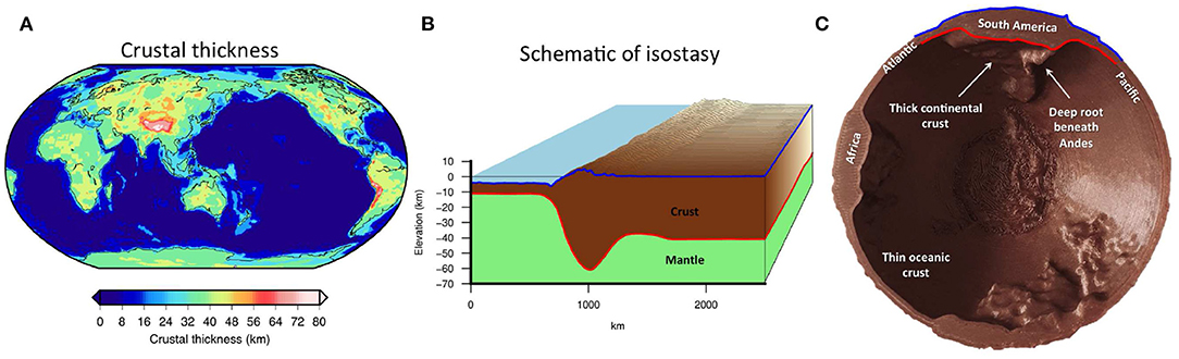
Figure 4. Crustal thickness globe. This globe shows how the crustal thickness (A) varies between oceans and continents, but also within continents. It can especially be used to illustrate the concepts of isostasy, i.e., how mountain ranges on the Earth are underlain by thick, deep crustal roots (B). The 3D-printed globe appears (C) identical to the Earth globe in Figure 3D, but can be opened to reveal the Moho and allow crustal thickness variations to be felt by hand.

Our crustal thickness globe is created from topographic variations (again using ETOPO1, Amante and Eakins, 2009; NOAA, 2009) and the Moho depth model from CRUST1.0 (Laske et al., 2013). Individual models of these parameters were created following the methodology described in section 2 and then combined using simple Boolean operations in Blender, such that the Moho globe was “subtracted” from the topography globe. The relief at the surface and on the base of the crust are at the same scale (50x vertical exaggeration), so that the extent of crustal roots can be directly compared to the surface topography. We created two versions of this model, one where the thickness of the crust is to scale, and a second where an additional constant thickness is added. This second version, which preserves the relative scale of topography at the surface and on the Moho, allows for the embedding of small magnets during printing, which enable the globe to be closed and opened up to reveal the Moho beneath the surface.

In addition to in structured teaching environments, these globes are also useful for public engagement, as the differences between oceans and continents, as well as the principle of isostasy can be introduced. As both surface and Moho topography are given on the same scale, the public can literally feel the crustal thickness variations by hand. For the same reasons, this globe would therefore be of particular utility when teaching these concepts to the visually impaired, though we have not yet tested this in practice.

3.2.2. Earth's Interior

Beneath the thin crustal layer, the Earth consists of a thick rocky mantle above the metallic liquid outer core and solid inner core. We have developed a scale model of these layers that is useful for explaining Earth's radial structure and visualising the relative size of the mantle and core. In our experience, demonstrating this globe often leads to discussions about how we know this radial structure, providing a natural introduction into the importance of seismology for imaging Earth's interior.

The 3D-printed Earth interior globe consists of 3 layers: the mantle, the outer core, and the inner core (Figure 5). We once again include surface topography from ETOPO1 on the outer layer, so that when closed, the globe appears identical to the standard Earth topography and crustal thickness globes. Radii for the outer and inner core are taken from the PREM model (Dziewonski and Anderson, 1981), the Preliminary Reference Earth Model commonly used in seismology. Excess ellipticity is also included (though impossible to discern visually), but topography on either the core-mantle or inner core boundary is not considered as it remains largely unconstrained (e.g., deSilva et al., 2018; Koelemeijer, 2021). Again, small neodymium magnets are inserted during printing to allow the globes to remain intact when closed.

FIGURE 5

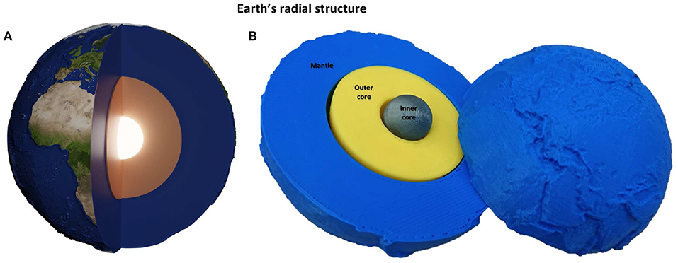
Figure 5. Earth interior globe. As depicted in cartoons of Earth's interior such as (A), this globe has multiple layers that can be taken apart and click together with magnets (B). This globe also appears identical to Figure 3D when closed. However, it can be opened up to illustrate the basic layered structure of the Earth, showing the mantle, outer core, and inner core.

This globe is particularly popular at public engagement events, with participants spending significant amounts of time engaging with it. By handling the Earth interior globe, people get a feel for how small the inner core really is. In addition, children of all ages enjoy taking the globe apart and putting it back together. Besides explaining the radial structure of the Earth, this globe can also be used together with our planetary teaching materials to relate the size of Mars and the Moon to the Earth: Mars is approximately the same size as the outer core while the Moon is just a little larger than the inner core. The globe also prompts a discussion about how we know Earth's interior structure and how recent the discoveries of the outer and inner core really are (Oldham, 1906; Lehmann, 1936). When displayed alongside 3D-printed globes of the Moon and Mars, the question naturally arises whether we can open up those globes too to reveal their internal structure. This facilitates discussion of the importance of space missions with seismic instruments to these planetary bodies to learn about their interior.

3.2.3. Seismic Tomography

The reworking of the Earth's surface is ultimately due to dynamic processes within our planet, as discussed in section 3.1. Within the rocky mantle, convection due to density variations provides the driving forces for the plate tectonic processes that have shaped the planet as we know it. Seismology allows us to study these dynamic processes and link them to surface features. Three-dimensional variations in seismic velocity (i.e., the velocity at which waves generated by earthquakes propagate through the Earth) are mapped using seismic tomography. These variations, often referred to as “velocity anomalies” relative to a reference velocity model, are caused by differences in temperature and chemical composition. However, these inherently 3D variations are difficult to visualise and often remain an abstract concept. By 3D printing seismic velocity variations at different depths, we can bring various seismological concepts to life and discuss the importance of seismology for understanding Earth's deep interior structure and processes.

Seismic velocity variations are taken from model SP12RTS (Koelemeijer et al., 2016), a whole mantle tomography model of shear- and compressional-wave velocity variations based on normal-mode, surface-wave and body-wave data. To make an intuitive link between surface processes and velocity structure we simply scale seismic velocity to 3D-printed topography (Figure 1), effectively interpreting velocity anomalies as being due to variations in temperature. Slow velocities are thus envisaged as hot, low-density, rising regions, e.g., domal swells over mantle plumes. Correspondingly, fast anomalies represent cold, high density, sinking material such as subducted plates. The 3D-printed globes thus gives an idea of where material moves upwards in a mantle upwelling and where plates subduct—thus linking plate tectonics with mantle convection. With this simple conceptual relationship, we represent depth slices of tomographic models as 3D-printable globes. Since SP12RTS is a long-wavelength model, we add a slight bump along velocity contours to aid visual interpretation, as can be seen in Figure 1C. As described in section 2, we give our globes geographic context by superimposing surface topography and coastlines.

In our seismic tomography globe (Figure 6), we nested globes of tomographic velocities at three different depths that can be opened like a Russian doll, fastened by embedded magnets. The resulting seismic “matryoshka” allows users to literally peel away different Earth layers and to discover how seismic structures change with depth (Figure 6E). We selected 3 depths at important boundary layers in the Earth: (1) 50 km depth, close to the surface, (2) 660 km depth, the top of the lower mantle, and (3) 2,850 km depth, the bottom of the lower mantle. The relative radii of the layers are schematic, as the requirement for them to nest would make surfaces intersect if scaled according to the correct radii in the Earth. At 50 km depth (Figure 6A), the most easily discernible features are cratons (high velocity, old, likely cold, so represented as depressions) and mid-ocean ridges (slow velocities, likely hot and upwelling, thus elevated), along with the difference between oceanic and continental lithosphere. At the top of the lower mantle (660 km depth), two fast regions (depressed topography) are observed below Southeast Asia and South America where deep subduction is occurring (Figure 6B). At 2,850 km depth, just above the core-mantle boundary, two large regions of very low velocities (elevated topography) are observed under Africa and the Pacific (Figure 6C). Although these two regions are elevated in our 3D-printed globes, thus portraying them as dominantly thermal structures, the nature of these Large-Low-Velocity-Provinces remains the subject of much research and intense academic debate (e.g., Garnero et al., 2016; Koelemeijer et al., 2017; McNamara, 2019).

FIGURE 6

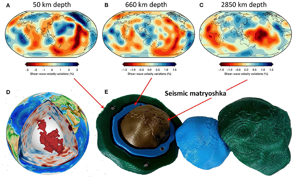
Figure 6. Seismic “matryoshka” globe. The seismic matryoshka depicts seismic velocity variations at different depths in the Earth's mantle: within the lithosphere (50 km depth, A), at the top of the lower mantle (660 km depth, B) and at the base of the lower mantle (2,850 km depth, C). While, 2D maps could be rendered in 3D on screen (as in D), the multi-layered 3D-printed globe (E) can be taken apart physically to explore features in different geographical locations. The globe is useful for explaining large-scale seismic structures and dynamic processes within the Earth to a more advanced audience.

Our seismic “matryoshka” globes can be used to discuss a range of topics in public engagement and teaching settings, from plate tectonics and mantle convection to planetary evolution. We find that initially, these globes cause some confusion as to what they are. However, they are intriguing enough that most people who handle them can grasp these complex concepts readily with guided questions. Using the globes, engagement with the topics is far higher than when shown the same data expressed as coloured 2D maps. Typical conversations begin with helping people discover what the “lumpy globes” represent and then lead to a discussion of the techniques we use to learn about the interior of the Earth, explaining the main concepts of global seismology. The specific features of each layer can also be discussed (as mentioned above), which help to convey concepts such as mantle convection and planetary cooling. The colours of the globes are chosen such that they reflect the dominant mineralogy at each depth: green at 50 km for olivine, blue at 660 km for ringwoodite, and gold/brown at 2,850 km for bridgmanite. We can thus ask what colour different regions in the Earth are, and explain what the colours mean. Finally, we can also talk about the factors that influence seismic velocities, what determines the velocity and how can we interpret these velocities?

We have so far largely used our seismic “matryoshka” globes at public engagement events and for undergraduate teaching. They are almost certainly too advanced to be used in primary schools, but they could be used in secondary school teaching packages and be linked to several aspects of the national science curriculum, such as the composition and structure of the Earth and the characteristics of sound waves (Key Stage 3, UK-Government, 2015). As the number of schools that offer geology courses and undergraduate enrolments at university have been declining (Boatright et al., 2019; Mosher and Keane, 2021), there is now a particular need for enhancing geosciences in school curricula through the introduction of new materials and activities, in order to spark the interest of students into geoscience from early years education.

3.2.4. A Game of Globes

While discussing the Earth's interior and displaying the models thus far described, both with school age pupils and at public engagement events, the most common question we have been asked is “How do we know what is inside the Earth?” To address this, we created a game that shows you do not need to be able to access the Earth's interior directly to be able to learn about it (Figure 7). We removed the core from globes of the Earth's interior (section 3.2.2) and replaced it with spheres of glass, steel and wood, a ping-pong ball and a scale model of Mars topography (which is coincidentally very close in size to the Earth's core). The audience is invited to shake the globes, feeling the weight and sensation of the objects moving inside and listening to the sounds they make, and then to make a guess as to what is inside. We use this game to draw analogy to what we can learn from the strength of the gravitational field and from “listening” to seismic waves that have passed through the Earth. Unfortunately, we are unable to report as to the efficacy of this game in practise; whilst we feel confident that it will be an excellent and engaging activity, the Covid-19 pandemic necessitated the cancellation of the 2020 Royal Holloway Science Festival at which we intended to trial it.

FIGURE 7

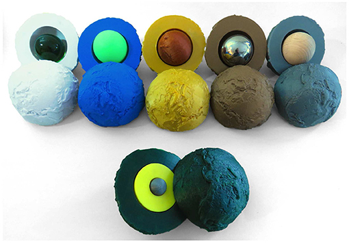
Figure 7. Game of globes. Spheres of different materials replace the core in 3D-printed globes of Earth topography. The audience is asked whether they can guess what is inside based on how heavy the globes are and the sound they make. This game can be used in a teaching or public engagement setting to illustrate how we can learn about the Earth's deep interior, using weight and sound as analogy to the gravitational field and seismology.

3.3. Other Scalar Fields

There are many other types of geophysical data besides topography and seismic tomography that provide insight into the Earth's interior and dynamic processes. Here, we briefly discuss two more fields that we have developed into 3D-printed globes, and what these may teach us about the Earth. However, our methodology can easily be applied to other fields, such as gravity or the magnetic field, or to explain more abstract concepts like spherical harmonics.

3.3.1. Dynamic Topography

Dynamic surface topography is caused by density variations and flow in the convecting mantle, perturbing the Earth's surface by ±1 km with wavelengths of 100s to 1000s km (e.g., Winterbourne et al., 2014). This is typically manifest as domal swells over warm, low-density, rising mantle and depressions over cold, dense sinking regions (Figure 8). Unlike more familiar sources of topography (crustal isostasy and flexure), it is not tectonically forced and changes through time as the convective interior of the Earth evolves. Understanding the pattern, wavelengths and scales of present day dynamic topography provides an important constraint on geodynamic modelling, explains patterns in sedimentation and erosion and provides an insight into mantle processes independent of seismology. As large datasets of reliable observations of dynamic topography have become available (e.g., Hoggard et al., 2017), it has become an increasingly important concept in both academia and industry.

FIGURE 8

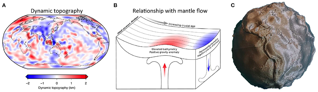
Figure 8. Dynamic topography globe. The observed pattern of present-day dynamic topography at the surface (A) provides information on density variations and mantle flow beneath the plates (B), reproduced from Winterbourne (2011). The 3D-printed globe (C) is useful in understanding the scale and shape of the anomalies, which are highly distorted near the poles in (A).

We use here the dynamic topography model of Hoggard et al. (2016). A vertical exaggeration of 300x gives a visually pleasing result in the 3D-printed globe, which we overlay with surface topography from ETOPO1. We again add a small artificial step at the coastline to make familiar coastlines easily recognisable. As the wavelengths of dynamic topography overlap with the wavelengths of topographic variations due to isostasy, we apply a spatial low cut filter to ETOPO1. This means that any long wavelength structure can be directly understood as being due to dynamic topography whilst the geographic context is still provided. The individual height maps of the 3D globe can be seen in Figures 2B–D.

Notable dynamic topographic highs are found at hotspots (e.g., Iceland, Hawaii). The rising low-density mantle that is responsible for hotspot volcanism also gives rise to large, long-wavelength topographic swells, which can be identified centred around the islands. Strong negative dynamic topographic anomalies are coincident with the Gulf of Mexico and the South Caspian basin. In these basins, the additional accommodation space available due to dynamic drawdown has allowed extremely thick piles of sediment to accumulate, in turn creating two of the world's most significant hydrocarbon systems. Examining the globe, it is immediately apparent that the signal is quite short wavelength, which implies that most of the variations originate in the shallowest part of the convecting mantle. Patterns also appear to not be restricted to tectonically active areas; for example, West Africa has large variations despite having been tectonically inactive since the Cretaceous period.

As a teaching aid, this globe is useful for explaining to undergraduate students the dynamic nature of the Earth's surface; constantly rising and falling above the turmoil of the convective interior. Natural questions often asked are how these anomalies form and how quickly they evolve (1s to 10s Ma), facilitating discussions of geological time scales and mantle dynamics. Therefore, it may also be appropriate for engaging with enthusiastic and well-informed members of the public.

It is interesting to compare the dynamic topography globe to the seismic tomography “matryoshka”: do we see the same patterns? Where do we see differences, and why? This allows discussion of the limitations of global tomographic resolution, which is poor in the asthenosphere where most of the causal density variations are inferred to be. It also enables us to discuss the difference between density structure (hard to constrain directly) and velocity anomalies, which do not correlate one-to-one with density as compositional variations also play a role.

3.3.2. Geoid

The geoid is an equipotential surface that represents the shape of the ocean surface due to variations in Earth's gravitational field and the theoretical extension of that surface onto land (Figure 9). It is usually expressed as a height anomaly relative to a reference ellipsoid (see Figure 9B). It was famously represented as a “3D” image informally known as the “Potsdam Potato” [e.g., see the excellent interactive website (Ince et al., 2019)] and served as an important inspiration for our 3D-printed globes concept. The geoid has been studied for centuries and provides geophysicists with information about the density structure of the Earth. Specifically, where there is a high density anomaly, gravity is slightly stronger and pulls the water toward it which creates a bulge at the surface—a “geoid high.”

FIGURE 9

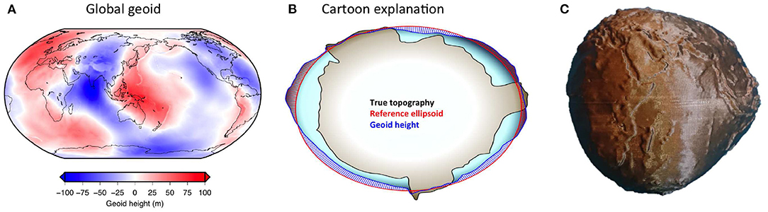
Figure 9. Geoid globe. Observations of the geoid (A) provide information on mantle density and viscosity. The geoid height shows the height of the equipotential surface (blue) of the Earth relative to the reference ellipsoid (red) in (B), and thus includes information on density at depth. Together with the Earth topography globe, the 3D-printed geoid globe (C) can be used to discuss the gravitational field and how it relates to density and viscosity variations in the deep Earth.

Our geoid globe is based on the EIGEN-6C4 model of Foerste et al. (2014). The geoid height anomaly is generally in the range of ±100 m, and our globe has a vertical exaggeration of approximately 10,000. Unlike our other globes, no surface topography is added for context. The geoid itself resembles surface topography at short wavelengths, reflecting the fact that mountains are much more dense than the air around them, which are thus associated with a locally high gravitational field strength. As with our other globes, a small artificial step has been added at the coastline, which is still useful for providing geographic context in areas with extensive continental shelves.

Together with the Earth topography globe, this geoid globe can be used in teaching settings to facilitate discussions on the gravitational field. A key observation to guide students toward is that the geoid is dominated by long wavelength structures and is thus sensitive to (and provides information on) density variations in the deep mantle. This fact can be contrasted with dynamic topography, which is dominated by much shorter wavelengths and sensitive to shallow structures in the upper mantle. Besides explaining the gravitational field, this globe can also be used to introduce the concept of viscosity within the convecting mantle, since the geoid is sensitive to both density and viscosity structure (e.g., Thoraval and Richards, 1997; Rudolph et al., 2015).

4. Discussion

In our Methodology section we have shown how 3D printed globes can be designed and manufactured, while the Results section documents how they can be used in teaching and public engagement settings to convey particular ideas and to stimulate specific conversations. In this section, we discuss the broader impact and limitations of our methodology, in the contexts of cost, practicality, sustainability and the feasibility of their use in a global pandemic.

4.1. Limitations of Our Methodology

4.1.1. Cost

We have striven to ensure that the cost to design and produce our globes is minimal. The workflow can be followed entirely in open source and free to use software and the designs are optimised to print using the minimal amount of material on the cheapest desktop printers available. We use (and recommend) polylactic acid (PLA) bioplastic filament, which can be sustainably produced from corn and has excellent properties for printing (low shrinkage, easy to print). PLA filament is available for as little as $20 per kilogram, meaning that even our largest and heaviest models, the seismic tomography matryoshkas, cost only around $5 in materials and energy usage.

Not every institution will have a 3D printer or cost-effective 3D printing service available, but these are already present in most universities and at an ever increasing number of schools. While the purchase cost of a basic printer (~$200) and the need for a competent operator should not be ignored, 3D printers can support many more educational activities and projects than our globes alone and so represent a reasonable investment for even small educational institutions.

4.1.2. Production Speed

3D printing is a relatively slow technique; each globe typically takes around 6 h to print. Our most complex models, the seismic matryoshkas, take even around 15 h due to the many layers. For creating sets of outreach materials that are used repeatedly at events, the time investment is manageable. However, for using these globes effectively in school settings, where 10 or more sets of globes might be required to run a single classroom session, printing time becomes the limiting factor. Consequently, our globes may be best suited to organisations such as university departments who run public engagement events at multiple schools.

4.2. Further Development

Going forward, we hope to provide freely accessible resources for schools that include a complete package of materials and a full lesson plan, building on previous efforts such as the Tactile Universe (Bonne et al., 2018) and following their recommendations for best practices. To form a complete teaching package that is both interactive and inclusive (Arcand et al., 2019), the globes are complemented by further materials, including demonstrator cheat sheets, animations, presentations, and paper materials (Figure 10). As an example of complementary paper materials, we designed and printed cut-out-and-fold dodecahedral globes of seismic tomography that matched the seismic matryoshka globes using code provided by Toussaint (2019). These handouts allowed the audience at our public engagement events to “take a globe home,” while also providing a medium for us to give links to online resources.

FIGURE 10

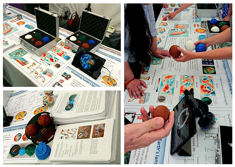
Figure 10. Impression of a public engagement event, where 3D-printed globes are used in conjunction with animations, information posters and handouts to inform the public about plate tectonics and seismic tomography.

4.3. Public Engagement During and After the Covid-19 Pandemic

The Covid-19 pandemic itself has recently created significant interest in seismology. Significant changes in anthropogenic seismic noise levels due to lockdowns and changes in behavioural patterns have been clearly recorded by seismometers (e.g. Lecocq et al., 2020) and received significant media and public interest. Whilst we are unable to directly capitalise on this interest by demonstrating our 3D models in person while the pandemic continues, our models and animations can be easily distributed online and be viewed in 3D using built-in tools on most modern operating systems (Arcand et al., 2020). They are therefore also suited for use in virtual classrooms, albeit with lessened impact. As restrictions on movements and events ease, we believe it will be possible to safely use our globes at in-person events. The PLA material used is resistant to isopropyl alcohol, which means the globes are easy to sterilise with a simple spray and cloth to combat the spread of the virus through surface contact.

5. Conclusions

3D visualisation and interpretation are very important in the Earth Sciences, but 3D concepts and patterns are not always easy to convey. In this contribution, we have shown how global scalar fields can be represented as cheap-to-produce 3D-printed globes. These globes are complementary to traditional 2D or digital methods of representing these fields, owing to their inherently 3D nature that avoids the inevitable distortions of map projections and provides an unbiased perspective on global fields. They are helpful in visualising complex global fields for audiences at all levels of knowledge and can make many geophysical properties accessible to the visually impaired.

In addition to presenting our methodology, we have presented numerous examples of our workflow applied in practice, creating globes of the topography of planetary bodies, crustal thickness, seismic tomography and dynamic surface topography. Along with the models, which we have made freely available, we have described the ideas and concepts that can be taught and explained using these globes, which we hope will prove useful for educators and science communicators. Our preliminary experiences of demonstrating our materials at events correlate with previous studies that found that 3D printed materials increase contact time at public engagement events and facilitate conversations about the underlying science.

Despite the current, temporary barriers to their use in schools and universities and at public engagement events, we are confident that our globes will offer excellent learning opportunities to audiences around the world. In particular, we hope that this easy-to-replicate method will make geophysical properties accessible to the visually impaired in a way that has not heretofore been possible.

Data Availability Statement

All our 3D-printable models are publicly available on Thingiverse (https://www.thingiverse.com/jeffwinterbourne/) while our workflow is documented with an example in the Supplementary Material and on our Github Repository (https://github.com/jeffwinterbourne/3D_globes).

Author Contributions

JW developed the 3D printing workflow and designed the 3D models. PK contributed data, concepts for models and created all teaching and outreach materials. Both authors contributed to the writing of the manuscript.

Funding

PK was funded by a Royal Society University Research Fellowship (URF\R1\180377) and gratefully acknowledges their support. Funding for 3D printing was also provided by an Enhancement Award from the Royal Society (RGF\EA\181029).

Conflict of Interest

The authors declare that the research was conducted in the absence of any commercial or financial relationships that could be construed as a potential conflict of interest.

Acknowledgments

We thank the Editor Max Rudolph and two reviewers, whose comments improved our manuscript. We are grateful to all authors and institutions who have provided and/or made freely available the data on which our models are based. Christophe Zaroli, Mark Hoggard, and Andreas Fichtner all helped us refine our models through discussion and feedback. Renaud Toussaint provided valuable discussion with regard to creating outreach and teaching materials. Sanne Cottaar made the initial suggestion for the game of globes. Angus Deveson and Joel Telling suggested the method for embedding magnets in models. We thank Dan McKenzie for his gift of a vacuformed 3D map of the geoid from 1974, which together with the Potsdam Potato inspired our 3D globe concept.

Supplementary Material

The Supplementary Material for this article can be found online at: https://www.frontiersin.org/articles/10.3389/feart.2021.669095/full#supplementary-material

Presentation 1. Step-by-step guide to 3D printing geophysical globes.

Data Sheet 2. Python notebook and example input files for generating 3D globes.

Data Sheet 3. Example output stl file part 1.

Data Sheet 4. Example output stl file part 2.

References

Airy, G. B. (1855). III. On the computation of the effect of the attraction of mountain-masses, as disturbing the apparent astronomical latitude of stations in geodetic surveys. Philos. Trans. R. Soc. Lond. 145, 101–104. doi: 10.1098/rstl.1855.0003

CrossRef Full Text | Google Scholar

Amante, C., and Eakins, B. (2009). ETOPO1: 1 Arc-Minute Global Relief Model: Procedures, Data Sources and Analysis. NOAA Technical Memorandum NESDIS NGDC-24.

Google Scholar

Arcand, K., Jubett, A., Watzke, M., Price, S., Williamson, K. T. S., and Edmonds, P. (2019). Touching the stars: improving NASA 3D printed data sets with blind and visually impaired audiences. J. Sci. Commun. 18, 16–20. doi: 10.22323/2.18040201

CrossRef Full Text | Google Scholar

Arcand, K. K., Price, S. R., and Watzke, M. (2020). Holding the cosmos in your hand: developing 3D modeling and printing pipelines for communications and research. Front. Earth Sci. 8:541. doi: 10.3389/feart.2020.590295

CrossRef Full Text | Google Scholar

Berman, B. (2012). 3-D printing: the new industrial revolution. Bus. Horizons 55, 155–162. doi: 10.1016/j.bushor.2011.11.003

CrossRef Full Text | Google Scholar

Boatright, D., Davies-Vollum, S., and King, C. (2019). Earth science education: the current state of play. Geoscientist 29, 16–19. doi: 10.1144/geosci2019-045

CrossRef Full Text

Bonne, N. J., Gupta, J. A., Krawczyk, C. M., and Masters, K. L. (2018). Tactile Universe makes outreach feel good. Astron. Geophys. 59, 1.30–1.33. doi: 10.1093/astrogeo/aty028

CrossRef Full Text | Google Scholar

Chickering, A. W., and Gamson, Z. F. (1987). Seven principles for good practice in undergraduate education. AAHE Bull. 3:7.

Google Scholar

Crameri, F., Shephard, G., and Heron, P. (2020). The misuse of colour in science communication. Nat. Commun. 11:5444. doi: 10.1038/s41467-020-19160-7

PubMed Abstract | CrossRef Full Text | Google Scholar

deSilva, S., Cormier, V. F., and Zheng, Y. (2018). Inner core boundary topography explored with reflected and diffracted P waves. Phys. Earth Planet. Interiors 276:202–214. doi: 10.1016/j.pepi.2017.04.008

CrossRef Full Text | Google Scholar

Dziewonski, A., and Anderson, D. (1981). Preliminary reference earth model. Phys. Earth Planet. Interiors 25, 297–356. doi: 10.1016/0031-9201(81)90046-7

CrossRef Full Text | Google Scholar

Foerste, C., Bruinsma, S., Abrikosov, O., Lemoine, J.-M., Marty, J. C., Flechtner, F., et al. (2014). EIGEN-6C4: The Latest Combined Global Gravity Field Model Including GOCE Data up to Degree and Order 2190 of GFZ Potsdam and GRGS Toulouse. GFZ Data Services.

Google Scholar

Ford, S., and Minshall, T. (2019). Invited review article: where and how 3D printing is used in teaching and education. Addit. Manufact. 25, 131–150. doi: 10.1016/j.addma.2018.10.028

CrossRef Full Text | Google Scholar

Garnero, E. J., McNamara, A. K., and Shim, S.-H. (2016). Continent-sized anomalous zones with low seismic velocity at the base of Earth's mantle. Nat. Geosci. 9, 481–489. doi: 10.1038/ngeo2733

CrossRef Full Text | Google Scholar

Hasiuk, F., and Harding, C. (2016). Touchable topography: 3D printing elevation data and structural models to overcome the issue of scale. Geol. Tdy 32, 16–20. doi: 10.1111/gto.12125

CrossRef Full Text | Google Scholar

Hasiuk, F. J., Harding, C., Renner, A. R., and Winer, E. (2017). TouchTerrain: a simple web-tool for creating 3D-printable topographic models. Comput. Geosci. 109, 25–31. doi: 10.1016/j.cageo.2017.07.005

CrossRef Full Text | Google Scholar

Hoggard, M., White, N., and Al-Attar, D. (2016). Global dynamic topography observations reveal limited influence of large-scale mantle flow. Nat. Geosci. 9, 456–463. doi: 10.1038/ngeo2709

CrossRef Full Text | Google Scholar

Hoggard, M. J., Winterbourne, J., Czarnota, K., and White, N. (2017). Oceanic residual depth measurements, the plate cooling model, and global dynamic topography. J. Geophys. Res. Solid Earth 122, 2328–2372. doi: 10.1002/2016JB013457

CrossRef Full Text | Google Scholar

Ince, E. S., Barthelmes, F., Reißland, S., Elger, K., Förste, C., Flechtner, F., et al. (2019). ICGEM - 15 years of successful collection and distribution of global gravitational models, associated services and future plans. Earth Syst. Sci. Data 11, 647–674. doi: 10.5194/essd-11-647-2019

CrossRef Full Text | Google Scholar

Ishutov, S., Jobe, T. D., Zhang, S., Gonzalez, M., Agar, S. M., Hasiuk, F. J., et al. (2018). Three-dimensional printing for geoscience: fundamental research, education, and applications for the petroleum industry. AAPG Bull. 102, 1–26. doi: 10.1306/0329171621117056

CrossRef Full Text | Google Scholar

Koelemeijer, P. (2021). Towards consistent seismological models of the core-mantle boundary landscape. Mantle Convection and Surface Expressions, Geophysical Monograph 263. doi: 10.1002/9781119528609.ch9

CrossRef Full Text | Google Scholar

Koelemeijer, P., Deuss, A., and Ritsema, J. (2017). Density structure of Earth's lowermost mantle from Stoneley mode splitting observations. Nat. Commun. 8, 1–10. doi: 10.1038/ncomms15241

PubMed Abstract | CrossRef Full Text | Google Scholar

Koelemeijer, P., Ritsema, J., Deuss, A., and Van Heijst, H.-J. (2016). SP12RTS: a degree-12 model of shear-and compressional-wave velocity for Earth's mantle. Geophys. J. Int. 204, 1024–1039. doi: 10.1093/gji/ggv481

CrossRef Full Text | Google Scholar

Laske, G., Masters, G., Ma, Z., and Pasyanos, M. (2013). Update on CRUST1. A 1-degree global model of Earth's crust. Geophys. Res. Abstr. 15:2658.

Google Scholar

Lecocq, T., Hicks, S. P., Van Noten, K., van Wijk, K., Koelemeijer, P., De Plaen, R. S. M., et al. (2020). Global quieting of high-frequency seismic noise due to COVID-19 pandemic lockdown measures. Science 369, 1338–1343. doi: 10.1126/science.abd2438

PubMed Abstract | CrossRef Full Text | Google Scholar

Lehmann, I. (1936). P'. Publications du Bureau Central Seismologique International A14, 87–115.

McNamara, A. K. (2019). A review of large low shear velocity provinces and ultra low velocity zones. Tectonophysics 760, 199–220. doi: 10.1016/j.tecto.2018.04.015

CrossRef Full Text | Google Scholar

Mosher, S., and Keane, C. (2021). Vision and Change in the Geosciences: the Future of Undergraduate Geoscience Education. Alexandria, VA: American Geosciences Institute. doi: 10.1130/abs/2020AM-355429

CrossRef Full Text

Müller, R. D., Cannon, J., Qin, X., Watson, R. J., Gurnis, M., Williams, S., et al. (2018). Gplates: building a virtual earth through deep time. Geochem. Geophys. Geosyst. 19, 2243–2261. doi: 10.1029/2018GC007584

CrossRef Full Text | Google Scholar

NOAA (2009). ETOPO1: 1 Arc-Minute Global Relief Model. NOAA National Centers for Environmental Information.

Google Scholar

Oldham, R. D. (1906). The constitution of the interior of the Earth, as revealed by earthquakes. Q. J. Geol. Soc. 62, 456–475. doi: 10.1144/GSL.JGS.1906.062.01-04.21

CrossRef Full Text | Google Scholar

Prince, M. (2004). Does active learning work? A review of the research. J. Eng. Educ. 93, 223–231. doi: 10.1002/j.2168-9830.2004.tb00809.x

CrossRef Full Text | Google Scholar

Rudolph, M. L., Lekić, V., and Lithgow-Bertelloni, C. (2015). Viscosity jump in Earth's mid-mantle. Science 350, 1349–1352. doi: 10.1126/science.aad1929

PubMed Abstract | CrossRef Full Text | Google Scholar

Smith, D., Zuber, M., Jackson, G., Cavanaugh, J. F., Neumann, G. A., Riris, H., et al. (2010). The lunar orbiter laser altimeter investigation on the lunar reconnaissance orbiter mission. Space Sci. Rev. 150, 209–241. doi: 10.1007/978-1-4419-6391-8_10

CrossRef Full Text | Google Scholar

Smith, D. E., Zuber, M. T., Frey, H. V., Garvin, J. B., Head, J. W., Muhleman, D. O., et al. (2001). Mars Orbiter Laser Altimeter: experiment summary after the first year of global mapping of Mars. J. Geophys. Res. Planets 106, 23689–23722. doi: 10.1029/2000JE001364

CrossRef Full Text | Google Scholar

Stauffer, R., and Zeileis, A. (2020). “Robust color maps that work for most audiences (including the US President,” in EGU General Assembly Conference Abstracts (Vienna), 7173. doi: 10.5194/egusphere-egu2020-7173

CrossRef Full Text | Google Scholar

Stuart, J., and Rutherford, R. D. (1978). Medical student concentration during lectures. Lancet 312, 514–516. doi: 10.1016/S0140-6736(78)92233-X

CrossRef Full Text | Google Scholar

Telling, J. (2019). Embedding Magnets When 3D Printing by Flipping Normals. Available online at: https://the3dprintingnerd.com/embedding-magnets-when-3d-printing-by-flipping-normals-thanks-to-makers-muse/

Thoraval, C., and Richards, M. A. (1997). The geoid constraint in global geodynamics: viscosity structure, mantle heterogeneity models and boundary conditions. Geophys. J. Int. 131, 1–8. doi: 10.1111/j.1365-246X.1997.tb00591.x

CrossRef Full Text | Google Scholar

Toussaint, R. (2019). renaud71/dodecahedron: Dodecahedron, Mapping of Spherical Data - First Release. Zenodo. doi: 10.5281/zenodo.2531114

CrossRef Full Text

UK-Government (2015). National Curriculum in England: Science Programmes of Study.

Google Scholar

Wessel, P., and Smith, W. H. (1996). A global, self-consistent, hierarchical, high-resolution shoreline database. J. Geophys. Res. 101, 8741–8743. doi: 10.1029/96JB00104

CrossRef Full Text | Google Scholar

Wessel, P., Smith, W. H. F., Scharroo, R., Luis, J., and Wobbe, F. (2013). Generic mapping tools: improved version released. EOS Trans. AGU 94, 409–410. doi: 10.1002/2013EO450001

CrossRef Full Text | Google Scholar

Winterbourne, J. (2011). Dynamic topography in the oceans (Ph.D. thesis). University of Cambridge, Cambridge, United Kingdom.

Google Scholar

Winterbourne, J., White, N., and Crosby, A. (2014). Accurate measurements of residual topography from the oceanic realm. Tectonics 33, 982–1015. doi: 10.1002/2013TC003372

CrossRef Full Text | Google Scholar