Impacts of Climate Change on Blue and Green Water Resources in the Xiangjiang River Basin of the Yangtze River, China

Highlights

1) The combination of future climate downscaling modeling with basin blue–green water modeling.

2) Revealing spatiotemporal variation of blue and green water components in the studied basin under historical and future climate change scenarios.

3) Using an improved parallel parameter calibration method to increase the accuracy of blue and green water simulations and decrease uncertainties.

4) Providing a basis for future blue and green water assessments at the basin scale and the general modeling framework can be applied to other regions with similar challenges.

1 Introduction

Many researchers have demonstrated in recent decades that climate change undoubtedly affects water resources worldwide (Haddeland et al., 2014; Reshmidevi et al., 2018). Consequently, assessing the impacts of climate change on water circulation and water resources at the basin scale is an important scientific issue (Sivapalan et al., 2011). In this context, it is more reasonable to link climate change and water resources according to water resource components, such as blue water and green water (Falkenmark and Rockström, 2010). Although the former has attracted widespread attention in many studies globally, the latter part needs further research in basin studies (Du et al., 2018).

Blue water and green water are both indispensable components of the hydrological cycle at the basin scale (Hoff et al., 2010; Keys and Falkenmark, 2018). The concept of blue and green water resources was initially proposed by Falkenmark (1995) at the Food and Agriculture Organization (FAO) Conference. Falkenmark and Rockstrom (2006) defined blue water resources, which are calculated based on the surface water yield (WYLD) and groundwater storage (GS), as liquid water in rivers, lakes, wetlands, and underground aquifers, whereas green water resources (Falkenmark and Rockstrom, 2010; Feng et al., 2020), which are estimated as the sum of evapotranspiration (ET) and soil water (SW), are divided into two components: green water flow (GWF) and green water storage (GWS). GWF, which refers to water vapor returned to the atmosphere through ET, is the potential water resource that benefits the ecosystem of the whole river basin and equals the actual ET, which comprises non-productive soil evaporation and productive plant transpiration (Cheng and Zhao, 2006). In contrast, GWS refers to the SW content (Rockström et al., 2009) contained within the upper unsaturated soil layers and is derived from the infiltration of precipitation, which is a potential source of GWF (Glavan et al., 2013).

On the continental scale, green water resources dominate the hydrological cycle, accounting for approximately 65% of the total amount of terrestrial blue and green water resources (Falkenmark and Rockström, 2010; Liu and Yang, 2010). Therefore, more precipitation returns to the atmosphere through soil evaporation and plant transpiration. Furthermore, green water is an important basis for agricultural production (Falkenmark, 2013), so it is indirectly consumed by humankind. Crops and trees predominantly rely on green water and sustain their growth by absorbing SW through transpiration, although irrigation (i.e., blue water) does play an important role. Hence, the green water cycle can improve and stabilize basin ecosystems (White et al., 2015) and provide terrestrial and aquatic ecological services (Kauffman et al., 2014) for nature and society.

Climate change may negatively impact freshwater circulation at the basin scale and further increase the uncertainties in the modeling of blue and green water resources (Vaghefi et al., 2014; Chen et al., 2014; Lee and Bae, 2015; Veettil and Mishra, 2018). Several blue and green water modeling studies have been performed in a few regions across China (Table 1). However, most of these studies have investigated the role of climate change in the variations in blue and green water resources under historical climate scenarios (e.g., Li et al., 2009; Liu et al., 2009; Xu., 2013; Zang and Liu, 2013; Zuo et al., 2015; Zhao et al., 2016; Xia et al., 2017; Lyu et al., 2019), whereas few publications have focused on the assessment of blue and green water variations and uncertainties at the basin scale under long-term future climate scenarios. In general, traditional basin water resource assessments pay inadequate attention to invisible green water resources (Hoff et al., 2010) and the impacts of future climate change, thereby underestimating the availability of water resources.

TABLE 1

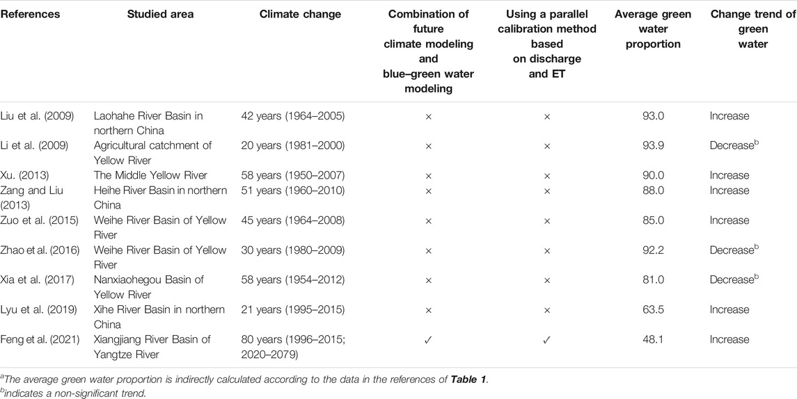
TABLE 1. Comparison of relevant studies in China evaluating the impacts of climate change on blue and green water resources at the basin scale.^a

Furthermore, previous studies in China have focused mostly on river basins located in northern China (characterized by arid or semiarid climates), such as the Yellow River (see Table 1), while only a few studies have been conducted on the Yangtze River Basin in southern China (characterized by a humid monsoon climate). In fact, the proportion of green water differs greatly between the Yangtze River (approximately 48.1% calculated within our studied basin, namely, the Xiangjiang River Basin) and the Yellow River (more than 80% as reported by previous papers) because the climate (e.g., precipitation) varies considerably between northern and southern China (Ye et al., 2013; Wang et al., 2021). Therefore, it is of practical significance to distinguish the blue and green water components (Mafuta, 2018) in a river basin characterized by a humid monsoon climate and to understand the implications of future climate change impacts on blue and green water resources (Abbaspour et al., 2009). These practices should improve water resource assessments in the studied basin and help establish a new approach for coping with water issues (such as water fluctuation, water scarcity, and water stress) (Rockström et al., 2015; Zhuo and Hoekstra, 2017) in other similar basins.

In addition, the surface runoff and ET processes of the basin water cycle are more complicated under the influence of climate change, and their effects vary in both space and time (Faramarzi et al., 2013; Rajib et al., 2018). Therefore, researchers have employed physical-based hydrological models (Zang and Liu, 2013) to replace the Budyko-based water balance methods (Budyko, 1974; Jiang et al., 2015), plant physiology methods (Postel et al., 1996; Rockström and Gordon, 2001), and traditional statistical methods based on the Penman–Monteith, Priestley–Taylor, and Hargreaves formulas (Xu, 2013; Vaghefi et al., 2014) to explore the transformation mechanism of blue–green water within the water cycle. Considering the differences in spatial scales, there are both global-scale models, such as the Lund–Potsdam–Jena managed Land (LPJmL) model, GIS-based Environmental Policy Integrated Climate (GEPIC) model, Global Water Resources H08 Model (H08), Global Crop Water Model (GCWM), and International Model for Policy Analysis of Agricultural Commodities and Trade (IMPACT) (Rockström et al., 2009; Hanasaki et al., 2010; Liu and Yang, 2010; Siebert and Doll, 2010; Robinson et al., 2015), and basin-scale models, such as the Soil and Water Assessment Tool (SWAT), Max Planck Institute Hydrology Model (MPI-HM), and Hydro-Informatic Modeling System Vegetation Impacts on Hydrology (HIM-VIH) (Chen et al., 2014; Abbaspour et al., 2015; Zuo et al., 2015; Liu et al., 2016).

However, the traditional blue and green water models not only ignore the selection and calibration of ET data but also use the default ET parameters of the model (Arnold et al., 2012; Badou et al., 2018). Hence, two questions arise: Can blue and green water components be accurately divided? Additionally, how can the spatiotemporal variations in blue and green water resources be predicted in the context of future climate change? These constitute two important scientific issues in the assessment of water resources in the Xiangjiang River Basin (XRB). Nevertheless, in practice, applying the concept of blue and green water to basin water resource assessments under future climate change remains difficult. These challenges include the combined modeling of future climate downscaling and basin-scale blue–green water resources (Reshmidevi et al., 2018; Farsani et al., 2019) and accurately identifying and quantifying blue and green water (Abbaspour et al., 2015; Zuo et al., 2015).

Therefore, in this study, an improved parallel parameter calibration method was adopted to simulate the generation and transformation of blue and green water components that consider both observed discharge data and remotely sensed ET data to increase the accuracy of blue and green water simulations and reduce uncertainties (Rajib et al., 2018; Kunnath-Poovakka et al., 2021). In general, this work presents an analytical study of the impacts of climate change on the past and the future division of blue and green water resources within the Xiangjiang River Basin. In combination with the SWAT hydrological model and the downscaling of general circulation models (GCMs), we analyze the temporal variations and spatial distributions of blue and green water resources in the context of climate scenarios based on four representative concentration pathways (RCPs), namely, RCP2.6, RCP4.5, RCP6, and RCP8.5, within four GCMs (HadCM3, IPSL-CM5A, HadGEM2-AO, and CCSM4). The results are expected to enrich the study of basin water resource assessments under future climate change and to provide references for the strategic formulation of integrated blue and green water resource assessments in the XRB and in other similar basins. Accordingly, the main goals of this study are to assess the proportions of the blue and green water components separately and to analyze the blue and green water variations under historical and future climate scenarios in the studied basin by employing an improved model calibration method.

2 Materials and Methods

2.1 Study Area Description

The XRB (94,660 km²), located in the Hunan Province of China between 24°38′N to 28°41′N latitude and 110°34′E to 114°15′E longitude, is a first-order tributary of the Yangtze River. The elevation of the basin ranges from −110 to 2,062 m, with an average of 302 m. The Xiangjiang River originates from Jinfengling Mountain in the Xingan County of Guangxi Province and has an overall length of 856 km. It flows from south to north through the cities of Yongzhou, Hengyang, Zhuzhou, Xiangtan, and Changsha into Dongting Lake and includes seventeen tributaries (the Liuyang River, Laodao River, Lianshui River, etc.). Moreover, the XRB is characterized by an East Asian subtropical humid monsoon climate; thus, its hydrological cycle also presents a monsoon climate regime. The average annual temperature in the XRB is between 18.0°C and 19.0°C, and its average annual precipitation ranges between 1,400 and 1,600 mm yr⁻¹, most of which falls from April to July. Accordingly, the flood season of the Xiangjiang River extends from April to July and accounts for approximately 52.4% of the annual runoff.

The XRB is of strategic importance for the water supply of Changsha (the capital of Hunan Province) and the Changsha–Zhuzhou–Xiangtan urban agglomeration (a national urban agglomeration in the middle reaches of the Yangtze River in China). The Xiangjiang River is also indispensable for agricultural irrigation; indeed, the XRB is one of the most important agricultural areas in the nation and thus has been called the “breadbasket of China.” Hence, research on assessing the water resources in the XRB is representative of Hunan Province, the Yangtze River, and even southern China. However, previous water resource assessments in the XRB focused exclusively on blue water. For example, the first comprehensive legislation on river basin protection in China, namely, the “Regulations on the Protection of the Xiangjiang River System” issued by the government of Hunan Province of China in 2013, is a kind of river water assessment rather than basin water assessment (Xiao et al., 2016). Because this legislation paid inadequate attention to the water cycle at the basin scale and neglected invisible green water, this practice (in addition to neglecting the impacts of future climate change) led to the water resources within the basin being underestimated. As a case study of the blue and green water resources in the XRB is representative of the Yangtze River (and even southern China), the XRB is selected as a representative basin to assess the impacts of climate change on the past and the future division of blue and green water resources.

The Xiangtan hydrometric station (a national control station of China) is the most important hydrological gauging station on the Xiangjiang River and includes a control river length of 738 km and a control catchment area of 81,638 km². In this paper, the catchment above the Xiangtan station was selected as the study area (81,638 km²), accounting for 86.24% of the total area of the XRB, as shown in Figure 1. This general map of the study area presents the modeling details and geographic distributions of the elevation, streams, watershed boundaries, climate stations, and discharge stations used in the hydrological model.

FIGURE 1

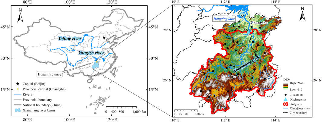
FIGURE 1. Location of the Xiangjiang River Basin, China.

2.2 Description of the Soil and Water Assessment Tool Model

SWAT is an integrated physical- and process-based distributed hydrological model (Arnold et al., 2013; Rathjens et al., 2015) specialized in analyses at the basin scale. Previous publications have demonstrated that the SWAT model can be computationally efficient when applied to characterizing the main processes of the water cycle, water quantity (surface runoff, baseflow, and stream flow), water quality (sediment load and nutrient flow), ET, and management practices (Keys and Falkenmark, 2018; Luan et al., 2018) in different landscapes (from small catchments to large river basins) at various spatial and temporal scales (Bieger et al., 2017).

The SWAT model has been extensively adopted for many international applications, e.g., the Savannah River Basin and Ohio River Basin in the United States (Veettil and Mishra, 2016; Du et al., 2018), Karkheh River Basin in Iran (Vaghefi et al., 2014), Cachoeira River Basin in Brazil (Rodrigues et al., 2014), Black Sea Basin (Rouholahnejad et al., 2014), Amazon River Basin (Lathuillière et al., 2016), Asian monsoon region (Lee and Bae, 2015), Europe (Abbaspour et al., 2015), Africa (Faramarzi et al., 2013; Mafuta, 2018), and the Heihe River Basin (Zang and Liu., 2013), Weihe River Basin (Zuo et al., 2015; Zhao et al., 2016), and Lianshui River Basin (Feng et al., 2017a) in China. Hence, SWAT is a valuable tool for investigating the different impacts of climate change on hydrological processes (Veettil and Mishra, 2016; Badou et al., 2018), as it provides spatial coverage of the entire hydrological cycle (Veettil and Mishra, 2018), including the atmosphere, plants, unsaturated zone, groundwater, and surface water. A more detailed description of the model is given in Section 3.

2.3 The Blue and Green Water Balance of the Soil and Water Assessment Tool Model

The water balance is the driving force that controls all the processes in the SWAT hydrologic model. The basic hydrological water balance equation used in the SWAT model can be expressed by Eqs 1, 2 (Arnold et al., 2013; Rodrigues et al., 2014; Farsani et al., 2019). In Eq. 1, PREC is the amount of precipitation (mm t⁻¹) during the time period t, ET denotes the actual evapotranspiration (mm t⁻¹) during the time period t (namely, GWF), and WYLD refers to the water yield (mm t⁻¹) during the time period t:

$\mathrm{PREC = ET}+\mathrm{WYLD}+\Delta \mathrm{SW}+\Delta \mathrm{GS+LOSSES},(1)$

$\mathrm{WYLD = SURQ+LATQ+GWQ}.(2)$

In Eq. 2, WYLD is the sum of surface runoff (SURQ, mm t⁻¹), lateral flow (LATQ, mm t⁻¹), and the groundwater contribution to streams (GWQ, mm t⁻¹), ΔSW represents the relative change in the soil water content (mm t⁻¹) (therefore, SW is equal to the amount of GWS, mm), ΔGS is the relative change in groundwater storage (mm t⁻¹) and is represented by the difference between GW_RCHG (the total amount of water recharge to aquifers) and GWQ within the SWAT output database, and LOSSES (mm t⁻¹) corresponds to the total losses of water interception and water transmission in the basin water cycle and the consumptive water use by human activities (domestic, industrial, or agricultural water use).

Therefore, the methodology and output parameters used in the SWAT model to calculate the blue and green water components are as follows: blue water (BW) = WYLD + GW_RCHG and green water (GW) = GWF + GWS = ET + SW (Arnold et al., 2013; Rodrigues et al., 2014; Veettil and Mishra, 2016). More details regarding the computation of WYLD, ET, and SW in SWAT can be found in the study by Feng et al. (2017b). The distributed structure of the SWAT model can efficiently characterize hydrological processes in catchments and distinguish the blue and green water components at the subbasin scale (Zhao et al., 2016; Veettil and Mishra, 2018). This model was therefore assumed to be suitable for the scenario analysis and simulation of blue and green water components across the XRB.

2.4 Climate Change Model and Scenario Design

The SWAT model, GCMs, and scenario analysis method (Faramarzi et al., 2013; Vaghefi et al., 2014; Lee and Bae., 2015; Badou et al., 2018) were used to project the impacts of climate change on blue and green water resources in the XRB. Analyses using GCMs and RCP scenarios from Coupled Model Intercomparison Project Phase 5 (CMIP5) might help further understand the impacts of climate change projections over the XRB. The SWAT model was forced by the historical climate scenario, scenario A (1996–2015), based on the observed meteorological conditions and by two future climate scenarios, scenarios B and C (2020–2049 and 2050–2079, respectively). These two future climate scenarios were generated from downscaled GCMs (HadCM3, IPSL-CM5A, HadGEM2-AO, and CCSM4) and four RCPs (RCP2.6, RCP4.5, RCP6, and RCP8.5). Accordingly, scenarios A, B, and C designed for this study are described as follows:

1) Scenario A (1996–2015). The baseline climate scenario was generated from meteorological data observed by weather stations from 1996 to 2015 in the XRB.

2) Scenario B (2020–2049). This scenario is subdivided into scenarios B2, B4, B6, and B8 according to RCP2.6, RCP4.5, RCP6, and RCP8.5, respectively, within the HadCM3, IPSL-CM5A, HadGEM2-AO, and CCSM4 models, which present the impacts of climate change in the near future for the period of 2020–2049.

3) Scenario C (2050–2079). Similar to scenario B, this scenario is subdivided into scenarios C2, C4, C6, and C8, which present the impacts of climate change in the far future for the period of 2050–2079.

2.5 Data Collection

The data required for this study were compiled from different sources as follows: 1) The ASTER Global Digital Elevation Model (GDEM) V2 at a 30 m spatial resolution was extracted from the Geospatial Data Cloud Site, Computer Network Information Center, Chinese Academy of Sciences, to delineate the topographic features of the XRB. 2) A land cover map with a spatial resolution of 300 m for 2015 was derived from the Data Center for Resources and Environmental Sciences (RESDC), Chinese Academy of Sciences. 3) Soil data were obtained from the Harmonized World Soil Database (HWSD) archived by the FAO of the United Nations and maps of China at a 1:1 million scale based on data distributed by the Institute of Soil Science in Nanjing, Chinese Academy of Sciences. 4) Historical weather input data of the total precipitation, average maximum/minimum air temperatures, wind speed, relative humidity, solar radiation, and meteorological statistics at 37 weather stations within the XRB from 1996 to 2015 were collected from the Climatic Data Center, National Meteorological Information Center, China Meteorological Administration. 5) Future weather input data for the period of 2020–2079 originated from four RCPs (RCP2.6, RCP4.5, RCP6, and RCP8.5) in four GCMs (HadCM3, IPSL-CM5A, HadGEM2-AO, and CCSM4) provided by the Fifth Assessment Report (AR5) of the Intergovernmental Panel on Climate Change (IPCC). 6) ET data were obtained from the MODIS16A2_ET product with a 0.05° spatial resolution for the period of 2000–2015; this product was available from the global terrestrial ET Moderate Resolution Imaging Spectroradiometer (MODIS) database of NASA. 7) Daily runoff data from 1996 to 2015 at the Xiangtan gauging station as well as a digital river network map, reservoir outflow data, water use data, and agricultural irrigation information of the study area were provided by the Hydrology and Water Resources Survey Bureau in the Hunan Province of China.

3 Model Inputs and Model Setup

3.1 Input Data Processing

3.1.1 Spatial and Attribute Data Processing

The 2015 land cover dataset was regridded to be consistent with the spatial resolution of the meteorological forcing data and then reclassified into eight classes according to the standard USGS land use and land cover categories used in the SWAT model, including 37.4% agricultural land (AGRL), 32.3% evergreen forest (FRSE), 10.1% deciduous forest (FRSD), 13.0% mixed forest (FRST), 1.7% shrubland (RNGB), 3.1% grassland (RNGE), 1.1% high-density residential urban land (URHD), and 1.3% water area (WATR), as shown in Figure 2.

FIGURE 2

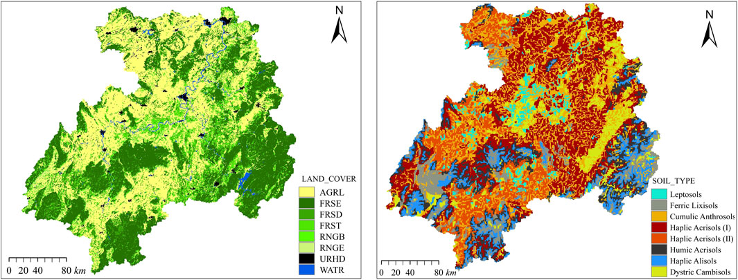
FIGURE 2. Land cover map and soil type map of the Xiangjiang River Basin.

As soil parameters have a significant influence on the simulation of green water, the soil database of the XRB was established based on the HWSD, the Soil-Plant-Air-Water (SPAW) model, and the soil statistical yearbook of Hunan Province (2010). The HWSD dataset contains most of the soil water information necessary for the SWAT model, such as two soil profiles (0–30 cm and 30–100 cm depths), the available water capacity, and the bulk density. The soil database was reclassified into eight classes of soil types used in the SWAT model, including 4.1% Leptosols, 7.4% Ferric Lixisols, 25.7% Cumulic Anthrosols, 26.2% Haplic Acrisols (I), 11.7% Haplic Acrisols (II), 10.2% Humic Acrisols, 7.5% Haplic Alisols, and 7.2% Dystric Cambisols, as shown in Figure 2.

Meteorological input data from 1996 to 2015 recorded at 37 weather stations in the XRB (including 57687-Changsha station, 57679-Changsha station, 57773-Xiangtan station, 57780-Zhuzhou station, 57872-Hengyang station, 57763-Loudi station, 57866-Yongzhou station, and 57972-Chenzhou station, among others), as shown in Figure 1, were selected to run the SWAT model; these data were also leveraged to help build the weather generator (WXGEN) (Aouissi et al., 2016) simultaneously. Then, historical climate change was simulated with SWAT by manipulating the climate inputs (WXGEN parameters, potential ET, precipitation, temperature, solar radiation, relative humidity, and wind speed) which were input into the model.

3.1.2 Future Climate Data and Their Downscaling

Four commonly used RCPs, namely, RCP2.6, RCP4.5, RCP6, and RCP8.5, were established by CMIP5 models from the IPCC AR5 corresponding to scenarios with a total radiative forcing of 2.6, 4.5, 6.0, and 8.5 W/m², respectively (approximately equal to mean CO₂ emission concentrations of 490, 650, 850, and 1,370 ppm), in 2100 (Diffenbaugh and Giorgi, 2012). To quantify the available blue and green water resources under future climate change (2020–2079), future climate projections from four GCMs (HadCM3, IPSL-CM5A, HadGEM2-AO, and CCSM4) under the RCP2.6, RCP4.5, RCP6, and RCP8.5 scenarios were fed into the SWAT model and were used as the future meteorological conditions.

Furthermore, a key issue in the combination of hydrologic models with GCMs is the spatial and temporal downscaling of the results from the latter. GCM outputs (Reshmidevi et al., 2018; Pandey et al., 2019) cannot be directly applied to the spatial resolution (Lee and Bae., 2015; Badou et al., 2018) of blue and green water modeling at the basin scale, so they must be downscaled to an acceptable spatiotemporal resolution. Accordingly, the climate change data for two future periods (2020–2049 and 2050–2079) were downscaled (Knutti and Sedlácek, 2012) and bias-corrected (Hassan et al., 2014) using the statistical downscaling model (SDSM) based on the observed meteorological records from the 37 nearest weather stations in the XRB for the baseline period (1996–2015). As a consequence, the downscaled climate series from HadCM3 agreed relatively well with the measured historical data. All 37 stations had R² values in the range of 0.81–0.89; hence, the downscaled HadCM3 model was identified as a better model for the XRB than the other three selected GCMs (IPSL-CM5A, HadGEM2-AO, and CCSM4).

3.1.3 MOD16 Data Processing

Given the high spatial variability in ET, satellite-derived MODIS16A2_ET data were used as the monthly average ET input for the model. This practice could achieve a better accuracy for the green water simulation if we calculate the spatial distribution of the actual ground surface ET (AET). The Penman–Monteith equation is used by the MOD16 ET algorithm (Mu et al., 2011) for remote sensing inversion, and this equation considers soil moisture evaporation, plant transpiration, water surface evaporation, etc. The quality control parameters of MOD16 have been verified by evaporation flux tower data at the global scale (Autovino et al., 2016), and application studies in China (Zhang and Chen, 2017) have shown that the MOD16 dataset is suitable for studying ET at the basin scale throughout most of China.

Additionally, ArcGIS software was used to calculate 0.05° monthly average ET raster data of the MOD16 ET product at a subbasin level for the purpose of calibrating the SWAT parameters for green water, and the satellite estimates were strongly correlated with the simulated results, as depicted and explained in Section 4.1.2.

3.2 Simulation Protocol

3.2.1 River Network Calibration and Division of Subbasins and Hydrological Response Units

The control river network of the XRB extracted from the DEM was calibrated with a 1:250,000 digital drainage map of the XRB according to the streamflow direction matrix (Feng et al., 2017a). Then, this control river network was used to calibrate the input river network generated by the SWAT model, which can improve the stream network’s accuracy of the D8 algorithm (Arnold et al., 2013) within the TOPOAZ module of SWAT. The threshold of the subbasin area in the SWAT model was set at 167,500 hm² based on a comparative analysis (Koch et al., 2013) between the observed and simulated errors of the starting points of streams (Feng et al., 2017a) from the digital drainage map of the XRB. Therefore, the Xiangjiang watershed was divided into 25 subbasins, as delineated in Figure 3, and the dominant land use and soil types of each subbasin were assigned.

FIGURE 3

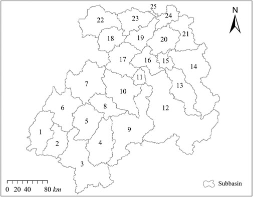
FIGURE 3. Spatial division of modeled units (subbasins) in the Xiangjiang River Basin.

It is recommended to reduce the computational burden by filtering unique combinations (Her et al., 2015). To spatially discretize each subbasin, SWAT utilizes hydrological response units (HRUs) which are delineated as the basis of the water balance calculation; this approach allows a subbasin to be split into unique combinations of soil, land use, and slope units. In this study, a 10% threshold of land use, soil, and slope that covered a fraction less than 10% of each subbasin was set up, which resulted in 382 HRUs distributed over 25 subbasins.

3.2.2 Model Calculation Method Setup

In this study, the surface runoff volume was simulated at the HRU level using a modified Soil Conservation Service (SCS) curve number (CN) procedure based on soil hydrologic groups, land use/land cover characteristics, antecedent soil moisture, etc. The variable storage method was used for routing the runoff aggregated from HRUs to each delineated subbasin and then routed to the associated reach and basin outlet through the river network. The FAO Penman–Monteith equation was selected to calculate the reference ET (Arnold et al., 2012; Aouissi et al., 2016). The leaf area index (LAI) and root development were estimated using the crop-growth component of SWAT, which is a simplification of the EPIC crop model.

3.2.3 Setup of Water Resource Use Scenario

Water use scenarios were set up within the SWAT model according to the average water use rate and domestic, industrial, and agricultural water use data in the XRB collected from the “Water Resources Bulletin of Hunan Province, China,” from 2006 to 2015. In addition, the outflow data of eight large-scale reservoirs in the study area, namely, the Centianhe Reservoir (2.50 billion m³ of flood control storage), Dongjiang Reservoir (1.58 billion m³), Taoshui Reservoir (1.00 billion m³), Shuifumiao Reservoir (0.70 billion m³), Ouyanghai Reservoir (0.62 billion m³), Shuangpai Reservoir (0.58 billion m³), Qingshanlong Reservoir (0.29 billion m³), and Jiubujiang Reservoir (0.11 billion m³), which may affect river discharge, were included in this model starting from 1996 to 2015. However, to study blue and green water variations under historical and future climate change scenarios in the long term (1996–2015 and 2020–2079), small reservoirs in the XRB were considered to mainly affect the daily runoff simulation in the flood season (Abbaspour et al., 2009; Ngo et al., 2016; Feng et al., 2017b) but have little effect on the monthly average river discharge calibration and validation.

Moreover, approximately 37% of the basin area is irrigated; therefore, the reservoirs listed above were built for agricultural irrigation districts downstream of the XRB. According to the operation scheme of gate dams in each reservoir and their annual average irrigated water volume, we set a corresponding irrigation management scenario in the model. Then, scenarios of water resource use and agricultural irrigation information were spatially parameterized (Dechmi et al., 2012; Rouholahnejad et al., 2014) for the model simulations within SWAT.

3.2.4 The Methodology of Blue and Green Water Modeling

Most previous studies on blue and green water simulations generally used the blue water calibration (discharge calibration) method in specific SWAT applications (Li et al., 2009; Arnold et al., 2012; Badou et al., 2018). Based on the observed discharge data and remotely sensed MODIS ET data (Feng et al., 2018; Rajib et al., 2018; Kunnath-Poovakka et al., 2021), this study used the particle swarm optimization (PSO) algorithm (Kennedy and Eberhart, 1995) in the SWAT-Calibration and Uncertainty Programs (SWAT-CUP) (Abbaspour et al., 2015) to simulate the blue and green water components (discharge and ET) simultaneously and characterize the overall uncertainty in the model output. The PSO algorithm and the Kling–Gupta efficiency (KGE) objective function in the SWAT-CUP were further applied to the sensitivity analysis, parameter estimation, and uncertainty quantification in this study. Based on the SWAT-CUP used in this study, the specific SWAT application was simultaneously combined and calibrated with the river discharge data (observed river discharge at the Xiangtan station) and basin ET data (MOD16 ET data at the subbasin scale) in the KGE objective function during model simulation, thereby providing a more reliable estimate of the coupling mechanism between blue and green water resources in a river basin. Ideally, the best simulation was calibrated with the largest objective function value.

3.3 Sensitivity Setup and Analysis

Compared with predicting the runoff in a river basin, calibrating the blue and green water resources is more complicated and must consider extra parameters (Abbaspour et al., 2015; Aouissi et al., 2016; Kundu et al., 2017) related to green water resources. Therefore, the sensitive parameters that control the calibration of runoff and ET calibration (and hence the calibration of blue and green water resources) in the basin should be identified.

In this study, the t-stat and p-value of Latin hypercube sampling one-factor-at-a-time (LH–OAT) (Kucherenko et al., 2011) and global sensitivity analysis within the SWAT-CUP (Abbaspour, 2014) were used to estimate the statistical significance of the parameters. The greater the absolute value of the t-stat is, the more sensitive the parameter is. Generally, the parameter is not sensitive at t < 0.05, weakly sensitive at 0.05 < t < 0.2, generally sensitive at 0.2 < t < 0.5, very sensitive at 0.5 < t < 1.0, and extremely sensitive at t > 1.0 (Mengistu and Sorteberg, 2012; Abbaspour, 2014; Zhao et al., 2016).

The selection of model parameters to calibrate was based on the sensitivity analysis and previous studies (Feng et al., 2017b and 2018). Based on an evaluation criterion, that is, t > 0.2, the 18 most sensitive hydrologic parameters within SWAT related to discharge and ET (blue and green water) within the XRB were identified, as shown in Table 2. In this study, these blue and green water parameters were employed to assess the blue and green water variations and to reflect the changes among the scenarios.

TABLE 2

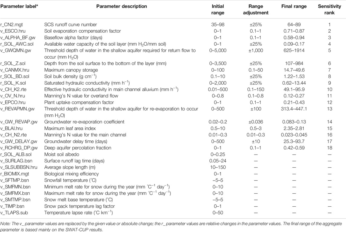
TABLE 2. Results of the sensitivity analysis and SWAT calibration procedure (the initial range, range adjustment in calibration, and final range) for the blue and green water parameters in the Xiangjiang River Basin.

3.4 Model Uncertainty Setup and Description

Blue and green water simulations contain uncertainties associated with the input data, model parameters, etc. This study used the parallel PSO algorithm (Kennedy and Eberhart, 1995) in the SWAT-CUP to characterize the overall uncertainty in the model output. In this method, all uncertainties are mapped onto the parameter ranges as the procedure attempts to capture most of the measured data within the 95% parameter prediction uncertainty (95 PPU) range (Abbaspour, 2014; Abbaspour et al., 2015).

Accordingly, the goodness of the model calibration strength and prediction uncertainties was judged by two indices, the p-factor and r-factor, of the 95 PPU. The p-factor indicates that the percentage of measured data falls in the 95 PPU band and varies from 0 to 1, where 1 is the maximum value of the p-factor, that is, 100% bracketing of the observed data by the 95 PPU (Rouholahnejad et al., 2014). In contrast, the r-factor represents the average width of the 95 PPU band divided by the standard deviation of the observed data and ranges from 0 to infinity, where a lower value of the r-factor indicates better model performance.

Ideally, we would like to bracket most of the measured data (plus their uncertainties) within the 95 PPU band (p-factor value tending to 1) and to have a narrow 95 PPU band (r-factor value close to 0) because these conditions signify a more reliable model. Generally, when the p-factor value is greater than 0.5 and the r-factor value is less than 1.5, the simulation uncertainty is believed to be covered within the confidence region. Furthermore, the simulation uncertainty is accepted to be within the desirable range when the p-factor value is greater than 0.7 and the r-factor value is less than 1 (Abbaspour, 2014; Abbaspour et al., 2015; Feng et al., 2018).

In addition, the KGE, an improved parameter calibration method proposed by Gupta et al. (2009), was used as the objective function for the SWAT model calibration. To compare the measured and simulated discharge and ET, the simulation performance of the SWAT model was evaluated by using the following goodness-of-fit criteria: the coefficient of determination (R²) between the measured and simulated data, Nash–Sutcliffe efficiency (NSE, which indicates the variance ratio of the simulated value to the measured data), and bias percentage (PBIAS, representing the overall trend in which the simulation value deviates from the measured data).

R² and NSE values close to 1 indicate good correspondence between the two series, and values between 0.7 and 1 are considered optimal for validating models on observations. In contrast, as the PBIAS tends toward 0, the simulation results become more representative. Relevant studies (Arnold et al., 2013; Koch et al., 2013; Abbaspour, 2014; Abbaspour et al., 2015; Daggupati et al., 2015; Zuo et al., 2015; Zhao et al., 2016; Veettil and Mishra, 2018) have shown that blue and green water simulations are credible when R² > 0.6, NSE > 0.6, PBIAS < 15%, and KGE > 0.7, and the simulation results are relatively good when R² > 0.8, NSE > 0.8, PBIAS < 5%, and KGE > 0.9. The preprocessing of the SWAT model input data was accomplished mainly in ArcGIS 10.3 and ENVI 5.3. More details on the model inputs and model setup, sensitivity setup and analysis, and uncertainty setup and description can be found in the studies of Abbaspour (2014), Feng et al. (2017b), and Feng et al. (2018).

4 Results and Discussion

4.1 Model Calibration, Validation, and Uncertainty Analysis

4.1.1 Design of the Calibration–Validation Period

The overall calibration and validation period selected in this study was 1996–2015. Different from the traditional calibration–validation method (Abbaspour et al., 2009; Rodrigues et al., 2014), we adopted the validation–calibration method (i.e., in reverse order) (Vaghefi et al., 2014; Feng et al., 2017b) to divide the validation period (1996–2005) and calibration period (2006–2015). Because this method might be conducive to the prediction of future blue and green water resources, it was proposed based on the following considerations.

1) The input scenarios within the SWAT model were performed by using the land cover scenario in 2015 and water use scenarios in 2006–2015. Therefore, we selected the calibration period 2006–2015 to match the time series of the input scenarios to interpret the model parameters and simulation process more properly. Accordingly, the future blue and green water resources within the XRB were simulated under future climate change scenarios, but the constant land cover scenario did not consider future land use conditions. This practice controls the current input land cover scenarios within the SWAT model, which could allow the modeled future blue–green water resources to be more properly interpreted under future climate projections. In this way, the uncertainties of future blue–green water projections under future climate scenarios can be measured more precisely. Thus, the cumulative error of uncertainties from both future climate change scenarios and future land use change scenarios can be avoided. 2) Compared to the validation period (1996–2005), the calibration period (2006–2015) was closer to the simulation period (2020–2079) of future climate change. Therefore, the parameter calibration results were more suitable for predicting blue and green water resources in the long-term future. 3) The real-time sequence did not determine the selection of the calibration–validation period because the SWAT model considers mainly the input scenario (Koch et al., 2013; Rathjens et al., 2015; Bieger et al., 2017) in the calibration–validation period, not the time sequence.

In blue and green water modeling, the initial values of some green water parameters, such as the SW content, default to 0, which is inconsistent with the actual conditions of the basin water balance. To alleviate the influences of unknown initial parameters on the green water simulation, we set up three-year periods before the calibration and validation periods (1992–1995 and 2002–2005, respectively) as warm-up periods. Such warm-up periods can precisely initialize parameters (e.g., soil moisture) and properly simulate green water resources (Kundu et al., 2017). Then, the warm-up periods were excluded from the simulation. The calibration and validation periods from 1996 to 2015 are described as follows: 1) During model calibration, 2006–2015 was set as the calibration period and 2003–2005 was set as the model warm-up period. 2) During model validation, 1996–2005 was set as the validation period and 1992–1995 was set as the model warm-up period.

4.1.2 Uncertainty Analysis of the Improved Blue and Green Water Simulations

Most previous studies on the simulation of blue and green water resources generally used the blue water calibration method (Li et al., 2009; Arnold et al., 2012; Badou et al., 2018). Therefore, they focused mainly on calibrating discharge and then simply calculated the total green water according to the water balance equation. However, this approach may neglect to calibrate green water in the context of basin hydrologic processes, increasing the uncertainty of green water projections and making it difficult to distinguish GWF from GWS.

In fact, blue and green water simulations are different from traditional blue water simulations (Rouholahnejad et al., 2012; Aouissi et al., 2016). We recommend considering discharge and ET simultaneously to increase the prediction accuracy of green water and to diminish uncertainties (Feng et al., 2018; Rajib et al., 2018; Kunnath-Poovakka et al., 2021). Therefore, this study used an improved parallel parameter calibration method to simultaneously calibrate the discharge and ET (Rajib et al., 2018; Kunnath-Poovakka et al., 2021) and hence the blue and green water resources. This parallel calibration method combined river discharge with ET in the objective function during the model simulations, thereby providing a more reliable estimate of the coupling mechanism between blue and green water resources in the river basin. This approach could be an effective practice to improve the model simulation performance of green water to some extent.

In this study, the specific SWAT application was calibrated and validated simultaneously using monthly observed discharge (1996–2015) at the Xiangtan station located at the downstream end of the XRB (Figure 1) and MOD16 ET data (2000–2015) at the subbasin scale in the study area. At the same time, the PSO algorithm and KGE objective function in the SWAT-CUP were applied to the sensitivity analysis, parameter estimation, and uncertainty quantification. Ideally, the best simulation was calibrated with the largest objective function value. Furthermore, to assess the reliability of our model projection, Figure 4 is constructed to visualize the model calibration and validation performance of discharge and ET. The shaded range within Figure 4 indicates the 95 PPU range, which is used to express the combined confidence (Daggupati et al., 2015) of the blue and green water projections, including the uncertainties of the input data, climate variation, and hydrological model.

FIGURE 4

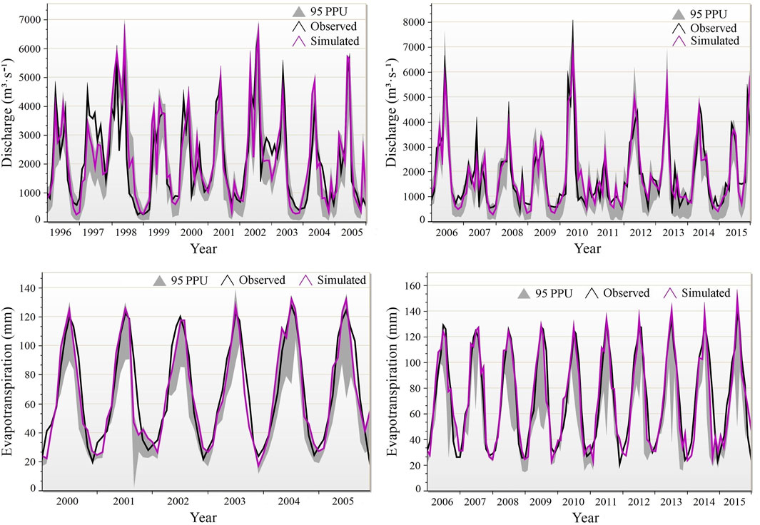
FIGURE 4. Simulation results and 95% parameter prediction uncertainty (95 PPU) ranges of the discharge and ET in the SWAT calibration (2006–2015) and validation (1996–2005) periods.

Based on the time-series plots between the simulated and observed values in Figure 4, the simulation performance coefficient and uncertainty analysis results within the calibration and validation periods are summarized in Table 3. As shown in Table 3, for all calibration and validation stages, the KGE statistic is greater than 0.85, R² is greater than 0.80, NSE is greater than 0.75, and PBIAS is less than 2.5%. The goodness of these KGE, NSE, R², and PBIAS coefficients (as discussed in Section 3.4) indicates reasonable agreement between the measured and simulated data. Therefore, compared to those of previous studies, the SWAT application results for the parallel simulation of discharge and ET during the calibration (2006–2015) and validation (1996–2005) periods were credible (Koch et al., 2013; Abbaspour et al., 2015; Zhao et al., 2016; Veettil and Mishra, 2018).

TABLE 3

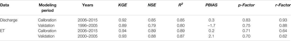
TABLE 3. Results of the simulated evaluation and uncertainty analysis of the discharge and ET in the SWAT calibration and validation periods in the Xiangjiang River Basin.

Referring to Table 3 for the calibration and validation periods of modeling, the p-factor values of the discharge and ET within the 95 PPU range are all greater than 0.70, indicating that, for the discharge and ET, more than 70% of the data are bracketed by the 95 PPU range. Likewise, all the r-factor values are below 0.95, indicating low prediction uncertainties for both the calibration and validation periods. According to the criteria of the uncertainty evaluation (p-factor greater than 0.7 and r-factor less than 1.5) recommended by Abbaspour et al. (2015), the uncertainties in the blue and green water simulations for the XRB conducted by the SWAT hydrological model were in the confidence area. As a consequence, the simulation performance of this hydrologic modeling by the improved parallel parameter calibration method in the XRB can be judged as satisfactory and hence can be applied to the spatiotemporal analysis of blue and green water in the basin.

4.2 Temporal Analysis of Blue and Green Water Under Climate Change Scenarios

The annual average values of blue water (BW) resources, green water flow (GWF), and green water storage (GWS) based on baseline scenario A (1996–2015), the four near-future climate scenarios B2, B4, B6, and B8 (2020–2049), and the four far-future climate scenarios C2, C4, C6, and C8 (2050–2079) are shown in Figures 5–7, respectively. We compared the relative differences among the eight future climate scenarios (B2, B4, B6, and B8 of 2020–2049 and C2, C4, C6, and C8 of 2050–2079) against baseline climate scenario A (1996–2015) and hence assessed the effects of different climate scenarios (Sections 4.2.1–4.2.4). Briefly, we analyzed the blue and green water projections under the best downscaled HadCM3 scenario in the XRB, as discussed in Section 3.1.2, while the IPSL-CM5A, HadGEM2-AO, and CCSM4 scenarios were used only to validate the confidence in the blue and green water predictions, as depicted in Figures 5–7, which show that almost all uncertainties in the blue and green water predictions plot within the 95 PPU ranges.

FIGURE 5

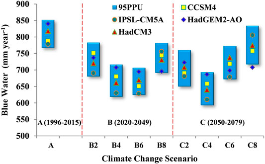
FIGURE 5. Annual average blue water resources in different climate scenarios simulated by baseline scenario A (1996–2015) and four GCMs (HadCM3, IPSL-CM5A, HadGEM2-AO, and CCSM4) in the Xiangjiang River Basin. Note: Future scenarios B (2020–2049) and C (2050–2079) are subdivided into climate scenarios B2, B4, B6, B8 and scenarios C2, C4, C6, C8 according to the four RCPs, RCP2.6, RCP4.5, RCP6, and RCP8.5, within the above four GCMs, as illustrated in Section 2.4; the terms in Figures 6, 7 are the same.

FIGURE 6

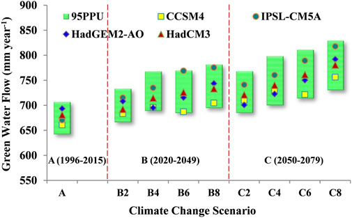
FIGURE 6. Annual average green water flow in different climate scenarios in the Xiangjiang River Basin.

FIGURE 7

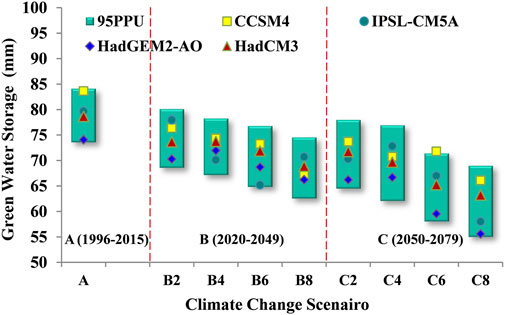
FIGURE 7. Annual average green water storage in different climate scenarios in the Xiangjiang River Basin.

4.2.1 Annual Variation in Blue Water Resources Under Different Climate Scenarios

Figure 5 shows the annual average BW over 20 years in the past (1996–2015) and 60 years in the future (2020–2049 and 2050–2079). The future changes in BW were calculated between the averages of scenarios B (2020–2049) and C (2050–2079) and that of baseline scenario A (1996–2015). Accordingly, 1) comparing scenario B (2020–2049) under RCP2.6, RCP4.5, RCP6, and RCP8.5 with scenario A (1996–2015; BW = 818.3 mm), BW shows different magnitudes of decline, with decreases of 97.9, 156.9, 148.7, and 87.2 mm, respectively. 2) Comparing scenario C (2050–2079) with scenario B (2020–2049) under RCP2.6 and RCP4.5, BW still shows dwindling trends, with decreases of 11.9 and 21.2 mm, respectively. However, the BW predictions in RCP6 and RCP8.5 are exceptionally large during scenario C (2050–2079), with increases of 68.1 and 43.6 mm, respectively. 3) The above analysis demonstrates that BW presents a decreasing trend when compared among all three climate periods of A, B, and C. In contrast with those in baseline scenario A (1996–2015), BW in the far-future scenario C (2050–2079) is predicted to decrease by 109.8, 178.1, 80.6, and 43.7 mm under RCP2.6, RCP4.5, RCP6, and RCP8.5, respectively, with reductions of approximately 5.3–21.8%.

Furthermore, a comparison between baseline scenario A and the future RCP scenarios shows that the decreasing trend of BW slows down successively from RCP2.6 to RCP4.5, RCP6, and RCP8.5. In other words, the larger the RCP number is (i.e., the greater the radiative forcing is), the smaller the reduction in BW is. The main reason for such differences may be that the regional atmospheric circulation and basin hydrological processes (e.g., precipitation, runoff) influenced by the different GCMs, different RCP scenarios, different CO₂ emission concentrations, and (more directly) the rainfall pattern and atmospheric temperature vary.

Especially under RCP6 and RCP8.5, BW is unexpectedly predicted to increase. This could be because the local precipitation and hence BW may increase in the mid-latitude areas, which are greatly affected by the intensification of global warming and monsoon circulation (Knutti and Sedlácek, 2012; Lee and Bae, 2015; Badou et al., 2018), e.g., the higher CO₂ concentrations of 850 and 1,370 ppm in the RCP6 and RCP8.5 scenarios, respectively, in 2100. The XRB is located exactly in the mid-latitude region and is characterized by a subtropical humid monsoon climate with typical monsoon climate properties, as discussed in Section 2.1. In general, climate change is predicted to reduce the BW within the XRB over the next 60 years (2020–2079), but these resources are expected to fluctuate according to different RCP scenarios and their future total radiation intensities and CO₂ emission concentrations.

4.2.2 Annual Variation in Green Water Flow Under Different Climate Scenarios

Figure 6 illustrates the annual average GWF based on the historical data of scenario A (1996–2015) and the future graphs of scenarios B (2020–2049) and C (2050–2079). 1) From historical scenario A (1996–2015; GWF = 680.9 mm) to future scenario B (2020–2049), GWF was predicted to show different growth rates under RCP2.6, RCP4.5, RCP6, and RCP8.5 with increases of 11.3, 33.7, 45.1, and 52.5 mm, respectively. 2) Moreover, from scenario B (2020–2049) to scenario C (2050–2079), GWF still shows an increasing trend, with increases of 28.9, 25.8, 35.4, and 47.3 mm. 3) In the comparison of baseline scenario A (1996–2015) with far-future scenario C (2050–2079), GWF is simulated to increase by 40.2, 59.5, 80.5, and 99.8 mm under the four different RCPs, which are equal to future growth rates of 5.9–14.7%.

Ultimately, the comparison among scenarios A, B, and C in Figure 6 indicates that the GWF under different RCPs exhibits a growth trend under the future climate background, and the larger the RCP emissions are, the greater the enhancement in GWF is. Similarly, the green water coefficient (equal to green water resources divided by blue–green water resources) was found to rise with an increase in GWF. By calculating the ratio of green water resources to blue–green water resources, the average green water coefficient (Falkenmark, 2013; White et al., 2015) is predicted to increase from 48.1% (average from 1996 to 2015) to 53.4% (average from 2050 to 2079).

The main reason for this enhanced GWF may be that ET increases with increases in the CO₂ emission concentration and temperature, whereas BW decreases slightly. As CO₂ emissions and temperatures increase, vegetation cover may become denser, and actual transpiration may rise. Simultaneously, soil evaporation, water surface evaporation, and groundwater re-evaporation may increase. This is because the XRB, located in an area with a subtropical humid monsoon climate (precipitation between 1,400 and 1,600 mm yr⁻¹), has diverse terrestrial and aquatic ecosystems with an extensive river network system and abundant surface water (e.g., lakes, reservoirs, ponds, paddy fields), soil water, and groundwater resources.

In addition, the GWF exhibited a growth trend even considering the 95 PPU range and the prediction results for four GCMs (HadGEM2-AO, IPSL-CM5A, HadGEM2-AO, and CCSM4), as presented in Figure 6. Although differences were discovered among the four GCM scenarios because of uncertainties and their underlying assumptions, the four GCM scenarios fell almost entirely within the predicted 95 PPU bands of the historical period (1996–2015) and future period (2020–2079). This implies that the increasing trend of GWF is highly credible under future climate scenarios in the XRB.

4.2.3 Annual Variation in Green Water Storage Under Different Climate Scenarios

Analyzing the different climate periods of scenarios A, B, and C in Figure 7 reveals a decreasing trend in GWS in each RCP. 1) A comparison of future scenario B (2020–2049) with historical scenario A (1996–2015; GWS = 78.7 mm) indicates that the GWF will decrease by 5.0, 4.9, 6.8, and 9.8 mm under RCP2.6, RCP4.5, RCP6, and RCP8.5, respectively. 2) Comparing scenario C (2050–2079) with scenario B (2020–2049), this decreasing trend is predicted to continue in scenario C, with decreases of 1.9, 4.1, 6.6, and 5.7 mm. 3) As a consequence, from scenario A (1996–2015) to scenario C (2050–2079), the GWS is simulated to decrease by 6.9, 9.0, 13.4, and 15.5 mm, diminishing on average by 8.8–19.7%.

Furthermore, even considering the 95 PPU range and the referenced GCMs (IPSL-CM5A, HadGEM2-AO, and CCSM4), a decreasing trend of GWS can be found. The increase in GWF (e.g., soil evaporation and plant transpiration) caused by future increases in the CO₂ emission concentration and temperature may explain the decline in GWS in the XRB. Accordingly, these findings provide convincing evidence emphasizing the negative relationship between GWF and GWS.

Moreover, the total annual GWS calculated simply by the accumulation of the 12 monthly amounts of GWS is considerably redundant. GWS represents soil moisture, which changes over time and may be affected by the initial soil water content. The output parameter “SW” (Veettil and Mishra, 2016; Kundu et al., 2017) within the SWAT model described in Section 2.3 actually represents the GWS at the end of a certain time period t. Therefore, the GWS illustrated above (Figure 7) represents the monthly average GWS summarized at the end of each month.

Above all, as depicted in Figures 5–7, the 95 PPU ranges of the predicted BW (82.4–117.1 mm), GWF (64.6–98.3 mm), and GWS (10.6–14.9 mm) differed under scenarios A, B, and C. The difference among the 95 PPU ranges may be attributed to the different simulated time scales of BW (annual), GWF (annual), and GWS (monthly), as explained above. Therefore, the 95 PPU range of the GWS simulation (10.6–14.9 mm) is the smallest. The fact that the 95 PPU range of BW (82.4–117.1 mm) is larger than that of GWF (64.6–98.3 mm) may be caused by the larger uncertainty in precipitation because BW is more sensitive than GWF to precipitation throughout the XRB.

4.2.4 The Division of Blue and Green Water Resources and Their Monthly Variation

The analysis of baseline climate scenario A spanning 1996–2015 (Figures 5–7) showed that blue and green water accounted for 51.9 and 48.1%, respectively, of the water resources in the XRB. Hence, the utilization potential of green water resources in the XRB is very important, and the total amount of blue and green water resources was estimated to be approximately twice the assessed amount of BW. Therefore, the green water proportion (48.1%) of the XRB (southern China) is far less than the green water proportion (more than 80%) in northern China, as reported in previous papers (Zang and Liu., 2013; Zuo et al., 2015; Zhao et al., 2016). The main reason for the large difference in the green water proportion between northern and southern China may be the distinct difference in the climate (e.g., precipitation).

In addition, this study also analyzed the monthly variations in blue and green water resources in the XRB during 1996–2015. As illustrated in Figure 8A, the blue water flow is greater during the flood season in the XRB, when rainfall is relatively abundant from April to July, amounting to 446.4 mm and accounting for 54.6% of the annual BW. This implies that BW has a good correlation with precipitation throughout the year. In other words, an increase in precipitation causes an increase in streamflow and hence BW. However, there is a time lag between the maximum precipitation during March–June and the maximum BW observed in April–July. This may be due to the surface runoff lag time (reflected by SURLAG.bsn) and groundwater delay time (reflected by GW_DELAY.gw) in the basin hydrological process. Furthermore, the maximum temperature and higher amount of ET reduce the peak runoff in July, which may be responsible for the lower amount of BW in July (accounting for only 17.8% of the total from April to July).

FIGURE 8

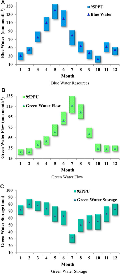
FIGURE 8. Distributions of the monthly average (A) blue water resources, (B) green water flow, and (C) green water storage simulated under historical climate scenario A (1996–2015) in the Xiangjiang River Basin.

A comparison of Figure 8B with Figure 8C shows that GWF gradually increases from January to June when GWS decreases and GWF continues to decline from July to December when GWS increases. Hence, GWF is negatively correlated with GWS throughout the year, indicating that GWS is a significant source of GWF. Specifically, GWS fell to the minimum value of 32.2 mm in July, when GWF reached its maximum value of 116.6 mm. The maximum value of GWF in July may be attributed to the higher temperature and precipitation during this period. Therefore, when the temperature increases, the actual ET (GWF) is also expected to increase, as demonstrated by Zang and Liu (2013), Veettil and Mishra (2016), Reshmidevi et al. (2018), and Farsani et al. (2019).

4.3 Impacts of Climate Change on the Spatial Distribution of Blue and Green Water

4.3.1 Spatial Distribution of Blue Water Resources

The spatial impacts of historical and future climate change scenarios (different RCPs within future HadCM3 scenarios under climate scenarios A, B, and C; see Section 2.4) were assessed on the subbasin scale, and blue and green water maps (Figures 9–12) were generated based on the subbasins and their representative values. The spatial distributions of BW under scenarios A (1996–2015), B (2020–2049), and C (2050–2079) are depicted in Figure 9 (historical period 1996–2015) and Figure 10 (future period 2020–2079). As shown in Figures 9, 10, at the subbasin scale, the amount of BW is different in the context of scenarios A, B, and C. However, at the basin scale for the whole XRB, the projected changes in BW exhibit similar spatial patterns under different climate scenarios and RCPs.

FIGURE 9

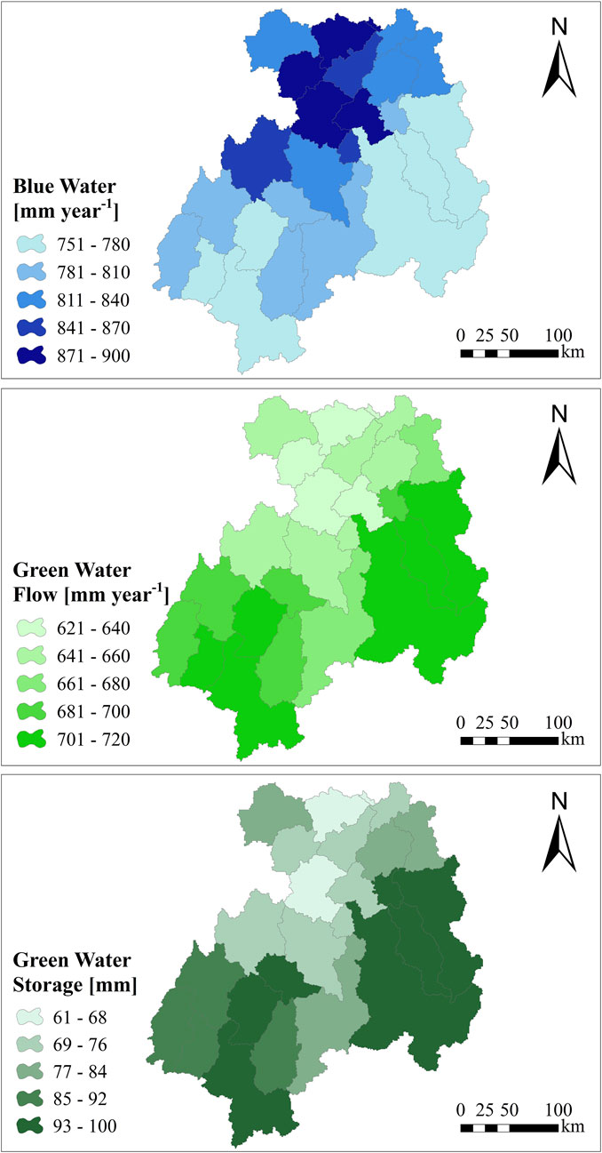
FIGURE 9. Spatial distributions of blue and green water resources under historical scenario A (1996–2015) in the Xiangjiang River Basin.

FIGURE 10

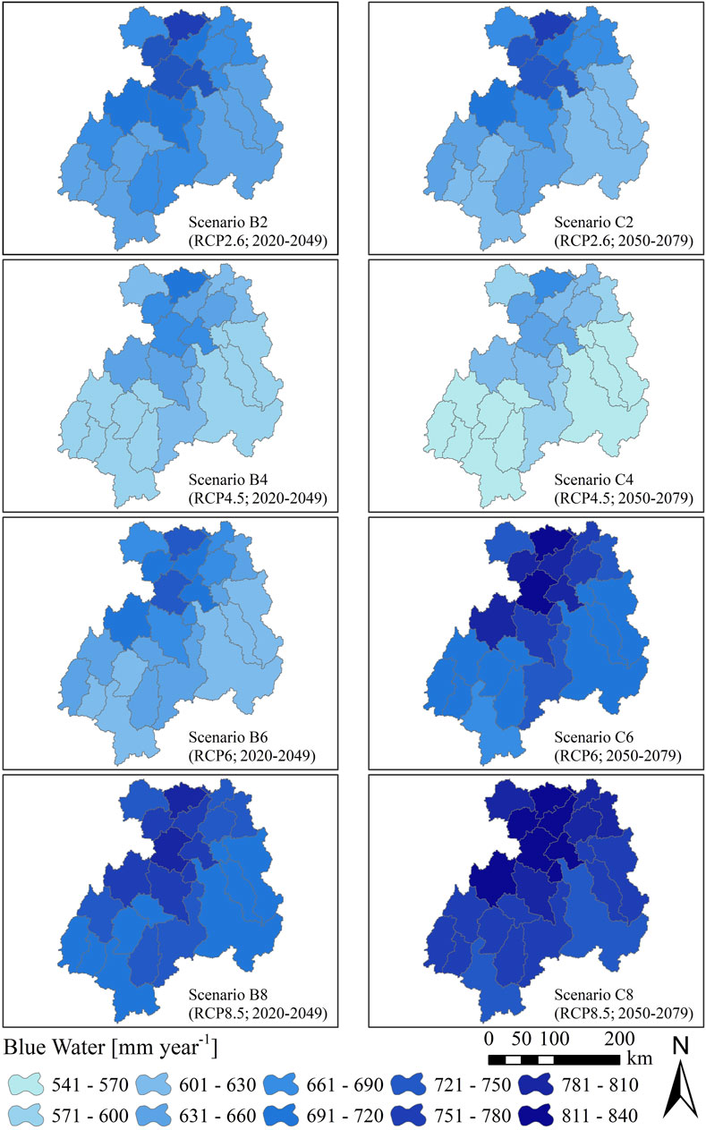
FIGURE 10. Spatial distributions of the annual average blue water resources (mm yr⁻¹) under different RCPs in future HadCM3 climate scenarios (2020–2079) in the Xiangjiang River Basin.

FIGURE 11

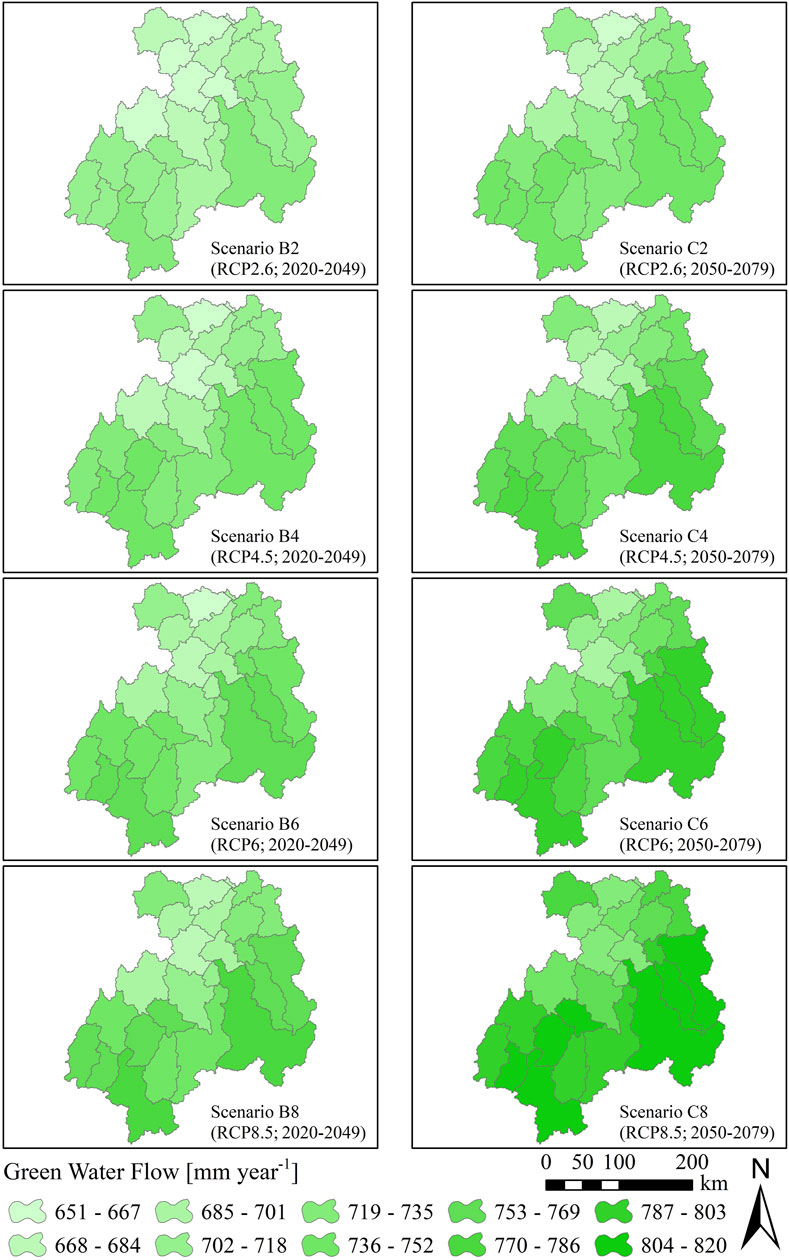
FIGURE 11. Spatial distributions of the annual average green water flow (mm yr⁻¹) under different RCPs in future HadCM3 climate scenarios (2020–2079) in the Xiangjiang River Basin.

FIGURE 12

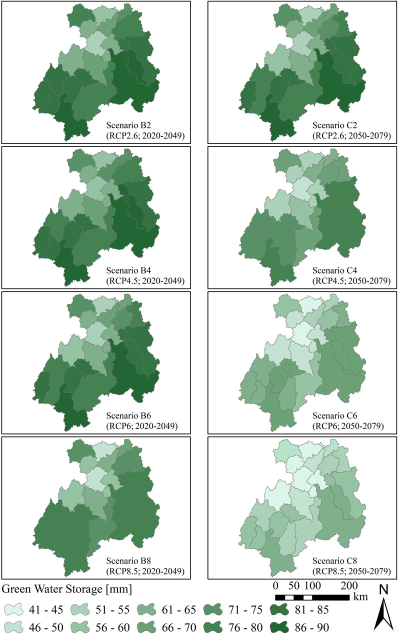
FIGURE 12. Spatial distributions of the annual average green water storage (mm yr⁻¹) under different RCPs in future HadCM3 climate scenarios (2020–2079) in the Xiangjiang River Basin.

Some previous studies have reported that the spatial distribution of BW is influenced mainly by the spatial pattern of precipitation (Veettil and Mishra, 2016; Farsani et al., 2019). Undoubtedly, taking climate change into account, an increase in precipitation will cause an increase in streamflow and hence BW (Reshmidevi et al., 2018). Therefore, at the subbasin scale, precipitation plays an important role in controlling the amount of BW under changing climate conditions (e.g., different amounts of BW among subbasins are shown in Figures 9, 10). However, at the basin scale, on the basis of Figure 3 (the spatial division of subbasins in the XRB), Figure 9, and Figure 10, the BW values downstream (subbasins 13–25 to the north) in the XRB are slightly higher than those upstream (subbasins 1–12 to the south) under different climate scenarios. In fact, the annual precipitation increases from downstream to upstream, as the precipitation depends mainly on the basin elevation and local climate characteristics of the XRB. Therefore, the spatial distribution of BW does not overlap with the spatial distribution of precipitation at the basin scale of the XRB.

The spatial differences between BW and precipitation at the basin scale of the whole XRB imply that BW is not only dependent on climate (e.g., precipitation) but also related to human activities (e.g., land use and land cover). In other words, BW is also influenced by the land use and land cover within the XRB. As depicted in Figures 9, 10, the subbasins with lower BW amounts (subbasins 1–6, 8–9, and 12–15 in the upstream and eastern areas of the XRB, as depicted in Figure 3) are spatially correlated with the forest area depicted on the land cover map (forest accounting for 55.4% of the XRB, as depicted in Figure 2). This indicates that relatively little BW exists within the forest cover of the XRB, while the amount of BW is much larger in agricultural and urban areas. Because forests can affect both land cover and soil permeability, precipitation may be more likely to permeate into the soil layer, thereby increasing the soil water content, soil evaporation, and plant transpiration. These factors all hinder the horizontal movement of water flow and surface runoff; therefore, BW may decrease correspondingly (Hoff et al., 2010; Hunink et al., 2012; Yang et al., 2016; Mafuta, 2018). According to the runoff dynamics of these areas, at the basin scale, this may explain why the spatial pattern of BW is relatively sensitive to the spatial distribution of land cover.

4.3.2 Spatial Distribution of Green Water Flow

The spatial distribution of GWF under different RCPs in scenarios A (1996–2015), B (2020–2049), and C (2050–2079) is plotted in Figures 9, 11. These two figures demonstrate that the three climate scenarios produce highly similar spatial patterns at the basin scale of the whole XRB, although the temporal results at the subbasin scale differ by varying degrees. At the basin scale, historical scenario A (1996–2015) and future scenarios B (2020–2049) and C (2050–2079) all show the same temporal increasing trend of GWF in the XRB, but there are spatial differences between the upstream (southern) and downstream (northern) parts. For example, Figures 3, 9, 11 show that the GWF value downstream (subbasins 13–25) is lower than that upstream (subbasins 1–12). In other words, more GWF is located in the upper part of the basin. This may be because the amount of GWF differs spatially depending on land use and land cover. The subbasins with relatively high GWF are spatially correlated with forest cover, such as subbasins 1–6, 8–9, and 12–15 in the upstream and eastern areas of the XRB, as shown in Figures 3, 9, 11, because more precipitation may permeate into the soil beneath forest cover and more soil moisture can be consumed by plants (e.g., plant transpiration), making precipitation more likely to be converted into GWF (Hunink et al., 2012).

However, in subbasins 7, 10–11, and 16–25, mostly located in the downstream part of the XRB, the GWF is relatively low and is found mainly on agricultural land, urban land, and their surrounding areas. This is in contrast to the spatial pattern of BW because the highly urbanized areas (e.g., the Changsha–Zhuzhou–Xiangtan urban agglomeration) and agricultural irrigated areas (e.g., the largest irrigation district of Shaoshan, approximately 67,000 ha) are located primarily in the downstream part of the XRB. Similarly, most farm crop production is cultivated predominantly in the downstream XRB, e.g., early-, middle-, and late-season rice, rapeseeds, beans, sweet potatoes, and vegetables. Compared to plants in forested areas, these crops may decrease the amount of GWF because of the lower crop transpiration and soil evaporation compensation factor (ESCO); similar findings were discussed by Liu and Yang (2010), Dechmi et al. (2012), and White et al. (2015).

Moreover, the amount of GWF in the forests (accounting for 55.4% of the XRB) is higher than that in the other land cover types; therefore, forest protection is the most effective measure for maintaining green water in the basin. However, agricultural land (accounting for 37.4% of the XRB) is also predominant; therefore, the soil evaporation and crop transpiration of farmland have important influences on controlling the GWF throughout the basin. In general, our findings suggest that, in addition to forest protection projects, improving the green water production efficiency (converting non-productive soil evaporation “E” into productive crop transpiration “T,” thereby raising the T/ET ratio) and developing the green water potential on farmland (Keys and Falkenmark, 2018) is also a feasible way to increase green water resources in the XRB. This practice needs to be given more attention in farmland management because this approach can balance blue and green water resources, which would have ecological service benefits for the whole basin.

4.3.3 Spatial Distribution of Green Water Storage

Figures 9, 12 indicate that the GWS in scenarios A (1996–2015), B (2020–2049), and C (2050–2079) in the downstream part of the basin (subbasins 13–25) is lower than that in the upstream part (subbasins 1–12). In other words, at the basin scale of the whole XRB, the GWS decreases from upstream (southern) to downstream (northern). Consequently, the spatial distribution of GWS is similar to that of GWF and different from that of BW. Similarly, this may be explained by the spatial correlation between green water and land cover (e.g., forest, agricultural, and urban lands), as discussed in Section 4.3.2. On the basis of Figures 3, 9, 12, we discover that the GWS in agricultural and urban areas (subbasins 7, 10–11, and 16–25, mostly in the downstream part of the XRB) is lower than that in forested areas (subbasins 1–6, 8–9, and 12–15 in the upstream and eastern areas of the XRB) under different climate scenarios and RCPs. Furthermore, the highly urbanized areas downstream (e.g., the Changsha–Zhuzhou–Xiangtan urban agglomeration) have the lowest GWS due to their lower soil depths, limited soil water supply, and predominantly impervious surface.

These results imply that the upstream and eastern areas of the XRB with greater GWS (or sufficient soil water) have a higher potential for the development of rainfed agriculture. Similar results have been reported for study areas in Iran (Faramarzi et al., 2009) and Europe (Abbaspour et al., 2015). Rainfed agriculture could be a good complement to the irrigation agriculture that already predominates in the XRB. In particular, compared with rainfed agriculture, irrigation farming may decrease blue water availability, intensify soil erosion, and deteriorate the ecological environment.

Furthermore, GWS is not only the main source of GWF but also related to green water production efficiency, reflected by the T/ET ratio, that is, green water productivity. In irrigation farmland, increasing the green water production efficiency (Kauffman et al., 2014; Zhuo and Hoekstra, 2017) can enhance productive crop transpiration while decreasing unproductive soil evaporation. In the XRB, agricultural land accounts for 37.4% of the area and is predominantly irrigation farmland. Therefore, in addition to developing rainfed farmland, measures of green water management (e.g., soil conservation, surface cover) for irrigation farmland are also favorable for improving the green water production efficiency throughout the XRB. From the perspective of game theory, implementing green water management is a positive-sum game that better utilizes green water availability and does not reduce BW (Feng et al., 2018).

5 Summary and Conclusion

This study carried out a modeling approach aimed at assessing the influences of historical and future climate change on blue and green water resources in the XRB, located along the Yangtze River of China. After parallel calibration and validation based on discharge and ET data, the SWAT model, four GCMs, and four RCP scenarios were applied to analyze the results. One historical climate scenario (1996–2015) and two future climate scenarios (2020–2049 and 2050–2079) were considered in this study. The hydrological modeling framework incorporating both discharge and ET data was found to be useful for quantifying the status of blue and green water resources within the XRB. Our results revealed the spatiotemporal distributions of blue and green water components and their uncertainties by simulating blue water (BW) resources, green water flow (GWF), and green water storage (GWS) in the context of climate change scenarios across the XRB:

1) An improved parallel parameter calibration method based on observed discharge data and remotely sensed ET data was used in this study. This method considers the selection and calibration of observed discharge data and remotely sensed ET data simultaneously to improve blue–green water modeling. The goodness of the coefficients (p-factor, r-factor, KGE, NSE, R², and PBIAS) in this study indicates a satisfactory performance of the blue–green water simulation in both the calibration and validation periods. Hence, this method could be effective for increasing the accuracy of blue and green water projections and for decreasing uncertainties in the studied basin, thereby providing more reliable estimates of the blue and green water components.

2) Regarding their temporal variations, the future blue–green water projections differed among the different future GCM scenarios and RCPs. The future BW and GWS in the XRB exhibit decreasing trends to varying degrees, whereas the GWF shows an increasing trend under the future climate background. From the perspective of uncertainty analysis, even if considering the 95 PPU range, the future trends of the predicted blue and green water components in this study are highly reliable. Although 95 PPU uncertainties were present in the simulated results, all climate scenarios predicted the future increasing trend in the green water proportion (an increase from 48.1 to 53.4% on average) for most regions of the XRB. Briefly, this study reveals relatively more pronounced effects of future climate change on green water (e.g., ET) than on blue water, which should be noted for the future water resource planning of the studied basin and other similar basins characterized by a humid monsoon climate. Therefore, integrating green water resources into the future water resource management of the XRB and comprehensively planning blue and green water resources are of practical significance.

3) Spatially, the blue–green water resources and land cover (e.g., forestland, agricultural land, and urban areas) show a good spatial correlation under all historical and future climate scenarios. We observed more green water (or less blue water) in the subbasins located in the upper parts of the basin, which could be related to the dense forest cover therein, whereas more blue water (or less green water) was noted in the subbasins in the lower parts of the basin, likely in association with the high degree of urbanization and widespread agricultural land. Hence, blue water and green water exhibit distinctive spatial patterns because of the land cover pattern in the whole XRB. According to the spatiotemporal analysis, we conclude that climate change mainly controls the temporal variations in blue and green water components in the XRB; therefore, future planning of blue and green water resources in the basin should take into account the influences of local climate change. However, climate change appears to have no significant impact on the spatial distribution of blue and green water at the basin scale of the whole XRB. Instead, land use and land cover are more likely to play an important role in the spatial distributions of blue and green water in the studied basin.

Overall, this study provides a basis for assessing blue and green water resources, and the general modeling framework utilized herein can be applied to other basins with similar challenges and may help decision-makers on a global scale. However, this study also has limitations. Uncertainties persist in the hydrological analyses, although we used a parallel parameter calibration method to decrease the uncertainties in the green water simulation. The modeling framework used to investigate the impacts of climate change on the blue–green water balance within the XRB may be affected by uncertainties in the input data (e.g., the deviation of the GCM projections and the MOD16 evapotranspiration data), model setup (e.g., the division of subbasins and HRUs), model parameters (e.g., not considering all blue and green parameters), calibration and validation, other modeling assumptions, and the uncertainty in the combination of the climate downscaling model with a basin hydrologic model.

Therefore, if the methods and results of this analysis of blue and green water in the XRB are directly applied to other watersheds of different sizes (i.e., smaller or larger basins), the uncertainties and scale effects of the blue and green water simulations should be carefully considered and addressed. In particular, the basin scale, climate conditions, land cover, and human activities of other watersheds might be different from those of the XRB. To conclude, there are four key issues to be addressed in our subsequent research: the evaluation of the simulated uncertainties and scale effect of blue and green water at different basin scales; the assessment of the potential impacts of blue and green water changes on water use by the agricultural, industry, and domestic sectors; the improvement of the combined effect of utilizing measured and remotely sensed data for calibrating the green water simulation; and the determination of the impacts of future human activities (e.g., future land cover change scenarios) on blue and green water.

Data Availability Statement

The raw data supporting the conclusion of this article will be made available by the authors, without undue reservation.

Author Contributions

CF prepared, created, and presented the published work; applied statistical, mathematical, computational, or other formal techniques to analyze or synthesize study data; and implemented the software and hydrological model. LY and CF conceptualized and formulated overarching research goals and aims; developed and designed the methodology; and was involved in project administration, and funding acquisition. LFH and CF curated, visualized, and presented the data. All authors were involved in critical review, commentary, and revision.

Funding

This study was financially supported by the National Natural Science Foundation of China (grant Nos. 42001024, 41901026, and 41807163), the National Key Research and Development Program of China (grant No. 2018YFC1508201), and the Natural Science Foundation of Hunan Province, China (grant No. 2021JJ40011).

Conflict of Interest

The authors declare that the research was conducted in the absence of any commercial or financial relationships that could be construed as a potential conflict of interest.

Publisher’s Note

All claims expressed in this article are solely those of the authors and do not necessarily represent those of their affiliated organizations, or those of the publisher, the editors, and the reviewers. Any product that may be evaluated in this article, or claim that may be made by its manufacturer, is not guaranteed or endorsed by the publisher.

Acknowledgments

Thanks are due to Professor Trevor Hoey from Brunel University London and Lecturer Georgios Maniatis from the University of Brighton for their assistance in this paper. The authors would also like to thank the handling editor, Professor Venkatesh Merwade, and two reviewers, Professors Adnan Rajib and Sayan Dey, for their reviews and valuable comments that significantly improved the quality of this paper.

References

Abbaspour, K. C. (2014). SWAT Calibration and Uncertainty Programs—A User Manual. Swiss. Dübendorf: Swiss Federal Institute of Aquatic Science and Technology.

Google Scholar

Abbaspour, K. C., Faramarzi, M., Ghasemi, S. S., and Yang, H. (2009). Assessing the Impact of Climate Change on Water Resources in Iran. Water Resour. Res. 45 (10), 434–449. doi:10.1029/2008wr007615

CrossRef Full Text | Google Scholar

Abbaspour, K. C., Rouholahnejad, E., Vaghefi, S., Srinivasan, R., Yang, H., and Kløve, B. (2015). A continental-scale Hydrology and Water Quality Model for Europe: Calibration and Uncertainty of a High-Resolution Large-Scale SWAT Model. J. Hydrol. 524, 733–752. doi:10.1016/j.jhydrol.2015.03.027

CrossRef Full Text | Google Scholar

Aouissi, J., Benabdallah, S., Lili Chabaâne, Z., and Cudennec, C. (2016). Evaluation of Potential Evapotranspiration Assessment Methods for Hydrological Modelling with SWAT-Application in Data-Scarce Rural Tunisia. Agric. Water Manage. 174, 39–51. doi:10.1016/j.agwat.2016.03.004

CrossRef Full Text | Google Scholar

Arnold, J. G., Kiniry, J. R., Srinivasan, R., and Williams, J. R. (2013). Soil and Water Assessment Tool Input/output File Documentation. Texas: Texas Water Resources Institute.

Google Scholar

Arnold, J. G., Moriasi, D. N., Gassman, P. W., Abbaspour, K. C., White, M. J., Srinivasan, R., et al. (2012). SWAT: Model Use, Calibration, and Validation. Trans. Asabe. 55 (4), 1491–1508. doi:10.13031/2013.42256

CrossRef Full Text | Google Scholar

Ashraf Vaghefi, S., Mousavi, S. J., Abbaspour, K. C., Srinivasan, R., and Yang, H. (2014). Analyses of the Impact of Climate Change on Water Resources Components, Drought and Wheat Yield in Semiarid Regions: Karkheh River Basin in Iran. Hydrol. Process. 28 (4), 2018–2032. doi:10.1002/hyp.9747

CrossRef Full Text | Google Scholar

Autovino, D., Minacapilli, M., and Provenzano, G. (2016). Modelling Bulk Surface Resistance by MODIS Data and Assessment of MOD16A2 Evapotranspiration Product in an Irrigation District of Southern Italy. Agric. Water Manage. 167, 86–94. doi:10.1016/j.agwat.2016.01.006

CrossRef Full Text | Google Scholar

Badou, D. F., Diekkrüger, B., Kapangaziwiri, E., Mbaye, M. L., Yira, Y., Lawin, E. A., et al. (2018). Modelling Blue and green Water Availability under Climate Change in the Beninese Basin of the Niger River Basin, West Africa. Hydrological Process. 32 (16), 2526–2542. doi:10.1002/hyp.13153

CrossRef Full Text | Google Scholar

Bieger, K., Arnold, J. G., Rathjens, H., White, M. J., Bosch, D. D., Allen, P. M., et al. (2017). Introduction to SWAT+, A Completely Restructured Version of the Soil and Water Assessment Tool. J. Am. Water Resour. Assoc. 53 (1), 115–130. doi:10.1111/1752-1688.12482

CrossRef Full Text | Google Scholar

Budyko, M. I. (1974). Climate and Life. Academic Press, 508.

Google Scholar

Chen, C., Hagemann, S., and Liu, J. (2014). Assessment of Impact of Climate Change on the Blue and green Water Resources in Large River Basins in China. Environ. Earth Sci. 74 (8), 6381–6394. doi:10.1007/s12665-014-3782-8

CrossRef Full Text | Google Scholar

Cheng, G. D., and Zhao, W. Z. (2006). Green Water and its Research Progresses. Adv. Earth Sci. 21 (3), 221–227. (in Chinese). doi:10.3321/j.issn:1001-8166.2006.03.001

CrossRef Full Text | Google Scholar

Daggupati, P., Yen, H., White, M. J., Srinivasan, R., Arnold, J. G., Keitzer, C. S., et al. (2015). Impact of Model Development, Calibration and Validation Decisions on Hydrological Simulations in West Lake Erie Basin. Hydrol. Process. 29 (26), 5307–5320. doi:10.1002/hyp.10536

CrossRef Full Text | Google Scholar

Dechmi, F., Burguete, J., and Skhiri, A. (2012). Swat Application in Intensive Irrigation Systems: Model Modification, Calibration and Validation. J. Hydrol. 470-471, 227–238. doi:10.1016/j.jhydrol.2012.08.055

CrossRef Full Text | Google Scholar

Diffenbaugh, N. S., and Giorgi, F. (2012). Climate Change Hotspots in the CMIP5 Global Climate Model Ensemble. Climatic Change 114, 813–822. doi:10.1007/s10584-012-0570-x

PubMed Abstract | CrossRef Full Text | Google Scholar

Du, L. Y., Rajib, A., and Merwade, V. (2018). Large Scale Spatially Explicit Modeling of Blue and Green Water Dynamics in a Temperate Mid-Latitude Basin. J. Hydrol. 562, 84–102. doi:10.1016/j.jhydrol.2018.02.071

CrossRef Full Text | Google Scholar

Fader, M., Gerten, D., ThammerHeinke, M. J., Heinke, J., Lotze-Campen, H., Lucht, W., et al. (2011). Internal and External green-blue Agricultural Water Footprints of Nations, and Related Water and Land Savings through Trade. Hydrol. Earth Syst. Sci. 8 (1), 483–527. doi:10.5194/hessd-8-483-2011

CrossRef Full Text | Google Scholar

Falkenmark, M. (1995). Coping with Water Scarcity under Rapid Population Growth. Pretoria, South Africa: Conference of SADC Minister.

Google Scholar

Falkenmark, M. (2013). Growing Water Scarcity in Agriculture: Future challenge to Global Water Security. Phil. Trans. R. Soc. A. 371, 20120410. doi:10.1098/rsta.2012.0410

PubMed Abstract | CrossRef Full Text | Google Scholar

Falkenmark, M., and Rockström, J. (2010). Building Water Resilience in the Face of Global Change: From a Blue-Only to a green-blue Water Approach to Land-Water Management. J. Water Resour. Plann. Manage. 136, 606–610. doi:10.1061/(asce)wr.1943-5452.0000118

CrossRef Full Text | Google Scholar

Falkenmark, M., and Rockström, J. (2006). The New Blue and green Water Paradigm: Breaking New Ground for Water Resources Planning and Management. J. Water Resour. Plann. Manage. 132 (3), 129–132. doi:10.1061/(asce)0733-9496(2006)132:3(129)

CrossRef Full Text | Google Scholar

Faramarzi, M., Abbaspour, K. C., Schulin, R., and Yang, H. (2009). Modelling Blue and Green Water Resources Availability in Iran. Hrydrol. Process 23, 486–501. doi:10.1002/hyp.7160

CrossRef Full Text | Google Scholar

Faramarzi, M., Abbaspour, K. C., Ashraf Vaghefi, S., Farzaneh, M. R., Zehnder, A. J. B., Srinivasan, R., et al. (2013). Modeling Impacts of Climate Change on Freshwater Availability in Africa. J. Hydrol. 480, 85–101. doi:10.1016/j.jhydrol.2012.12.016

CrossRef Full Text | Google Scholar

Fazeli Farsani, I., Farzaneh, M. R., Besalatpour, A. A., Salehi, M. H., and Faramarzi, M. (2019). Assessment of the Impact of Climate Change on Spatiotemporal Variability of Blue and green Water Resources under CMIP3 and CMIP5 Models in a Highly Mountainous Watershed. Theor. Appl. Climatol 136, 169–184. doi:10.1007/s00704-018-2474-9

CrossRef Full Text | Google Scholar

Feng, C., Mao, D. H., Zhou, H., Cao, Y. M., and Hu, G.W. (2018). Game Modeling and Application Analysis of green Water Management in the River basin. Resour. Environ. Yangtze Basin 27 (11), 2505–2517. doi:10.11870/cjlyzyyhj201811012

CrossRef Full Text

Feng, C., Mao, D. H., Zhou, H., Cao, Y. M., and Hu, G. W. (2017a). Impacts of Climate and Land Use Changes on Runoff in the Lianshui basin. J. Glaciology Geocryology 39 (2), 395–406. doi:10.7522/j.issn.1000-0240.2017.0045

CrossRef Full Text | Google Scholar

Feng, C., Mao, D. H., Yang, L., Zhou, H., and Hu, G.W. (2020). Research Progress and Commentary of Green Water Resources. Journal of Agricultural Resources and Regional Planning. 40 (1), 173–184. doi:10.7621/cjarrp.1005-9121.20200122

CrossRef Full Text

Feng, C., Yang, L., and Han, L. F. (2021). Impacts of Climate Change on Blue and Green Water Resources in the Xiangjiang River Basin of the Yangtze River, China. Front. Earth Sci. 9 (677191). doi:10.3389/feart.2021.677191

CrossRef Full Text | Google Scholar

Glavan, M., Pintar, M., and Volk, M. (2013). Land Use Change in a 200-year Period and its Effect on Blue and green Water Flow in Two Slovenian Mediterranean Catchments-Lessons for the Future. Hydrol. Process. 27 (26), 3964–3980. doi:10.1002/hyp.9540

CrossRef Full Text | Google Scholar

Gupta, H. V., Kling, H., Yilmaz, K. K., and Martinez, G. F. (2009). Decomposition of the Mean Squared Error and Nse Performance Criteria: Implications for Improving Hydrological Modelling. J. Hydrol. 377, 80–91. doi:10.1016/j.jhydrol.2009.08.003

CrossRef Full Text | Google Scholar

Haddeland, I., Heinke, J., Biemans, H., Eisner, S., Flörke, M., Hanasaki, N., et al. (2014). Global Water Resources Affected by Human Interventions and Climate Change. Proc. Natl. Acad. Sci. USA 111, 3251–3256. doi:10.1073/pnas.1222475110

PubMed Abstract | CrossRef Full Text | Google Scholar

Hanasaki, N., Inuzuka, T., Kanae, S., and Oki, T. (2010). An Estimation of Global Virtual Water Flow and Sources of Water Withdrawal for Major Crops and Livestock Products Using a Global Hydrological Model. J. Hydrol. 384 (3), 232–244. doi:10.1016/j.jhydrol.2009.09.028

CrossRef Full Text | Google Scholar

Hassan, Z., Shamsudin, S., and Harun, S. (2014). Application of SDSM and LARS-WG for Simulating and Downscaling of Rainfall and Temperature. Theor. Appl. Climatol 116, 243–257. doi:10.1007/s00704-013-0951-8

CrossRef Full Text | Google Scholar

Her, Y., Frankenberger, J., Chaubey, I., and Srinivasan, R. (2015). Threshold Effects in HRU Definition Ofthe Soil and Water Assessment Tool. Trans. Asabe. 58 (2), 367–378. doi:10.13031/trans.58.10805

CrossRef Full Text | Google Scholar

Hoff, H., Falkenmark, M., Gerten, D., Gordon, L., Karlberg, L., and Rockström, J. (2010). Greening the Global Water System. J. Hydrol. 384, 177–186. doi:10.1016/j.jhydrol.2009.06.026

CrossRef Full Text | Google Scholar

Hunink, J. E., Droogers, P., Kauffman, S., Mwaniki, B. M., and Bouma, J. (2012). Quantitative Simulation Tools to Analyze up- and Downstream Interactions of Soil and Water Conservation Measures: Supporting Policy Making in the green Water Credits Program of Kenya. J. Environ. Manage. 111, 187–194. doi:10.1016/j.jenvman.2012.07.022

PubMed Abstract | CrossRef Full Text | Google Scholar

Jiang, C., Xiong, L., Wang, D., Liu, P., Guo, S., and Xu, C. Y. (2015). Separating the Impacts of Climate Change and Human Activities on Runoff Using the Budyko-type Equations with Time-Varying Parameters. J. Hydrol. 522, 326–338. doi:10.1016/j.jhydrol.2014.12.060

CrossRef Full Text | Google Scholar

Kauffman, S., Droogers, P., Hunink, J., Mwaniki, B., Muchena, F., Gicheru, P., et al. (2014). Green Water Credits - Exploring its Potential to Enhance Ecosystem Services by Reducing Soil Erosion in the Upper Tana basin, Kenya. Int. J. Biodiversity Sci. Ecosystem Serv. Manage. 10 (2), 133–143. doi:10.1080/21513732.2014.890670

CrossRef Full Text | Google Scholar

Kennedy, J., and Eberhart, R. C. (1995). “Particle Swarm Optimization,” in Proceedings of IEEE International Conference on Neutral Networks (Perth, Australia.

Google Scholar

Keys, P. W., and Falkenmark, M. (2018). Green Water and African Sustainability. Food Sec. 10 (3), 537–548. doi:10.1007/s12571-018-0790-7

CrossRef Full Text | Google Scholar

Knutti, R., and Sedláček, J. (2012). Robustness and Uncertainties in the New CMIP5 Climate Model Projections. Nat. Clim Change 3 (4), 369–373. doi:10.1038/nclimate1716

CrossRef Full Text | Google Scholar

Koch, S., Bauwe, A., and Lennartz, B. (2013). Application of the SWAT Model for a Tile-Drained lowland Catchment in North-Eastern Germany on Subbasin Scale. Water Resour. Manage. 27 (3), 791–805. doi:10.1007/s11269-012-0215-x

CrossRef Full Text | Google Scholar

Kucherenko, S., Feil, B., Shah, N., and Mauntz, W. (2011). The Identification of Model Effective Dimensions Using Global Sensitivity Analysis. Reliability Eng. Syst. Saf. 96 (4), 440–449. doi:10.1016/j.ress.2010.11.003

CrossRef Full Text | Google Scholar

Kundu, D., Vervoort, R. W., and van Ogtrop, F. F. (2017). The Value of Remotely Sensed Surface Soil Moisture for Model Calibration Using SWAT. Hydrol. Process. 31, 2764–2780. doi:10.1002/hyp.11219

CrossRef Full Text | Google Scholar

Kunnath-Poovakka, A., Ryu, D., Eldho, T. I., and George, B. (2021). Parameter Uncertainty of a Hydrologic Model Calibrated with Remotely Sensed Evapotranspiration and Soil Moisture. J. Hydrologic Eng. 26 (3), 1–15. doi:10.1061/(asce)he.1943-5584.0002055

CrossRef Full Text | Google Scholar

Lathuillière, M. J., Coe, M. T., and Johnson, M. S. (2016). A Review of green- and Blue-Water Resources and Their Trade-Offs for Future Agricultural Production in the Amazon Basin: what Could Irrigated Agriculture Mean for Amazonia. Hydrol. Earth Syst. Sci. 20 (6), 2179–2194. doi:10.5194/hess-20-2179-2016

CrossRef Full Text | Google Scholar

Lee, M.-H., and Bae, D.-H. (2015). Climate Change Impact Assessment on green and Blue Water over Asian Monsoon Region. Water Resour. Manage. 29 (7), 2407–2427. doi:10.1007/s11269-015-0949-3

CrossRef Full Text | Google Scholar

Li, Z., Liu, W.-z., Zhang, X.-c., and Zheng, F.-l. (2009). Impacts of Land Use Change and Climate Variability on Hydrology in an Agricultural Catchment on the Loess Plateau of China. J. Hydrol. 377, 35–42. doi:10.1016/j.jhydrol.2009.08.007

CrossRef Full Text | Google Scholar

Liu, C. M., Li, Y. Z., and Liu, X. M. (2016). Impact of Vegetation Change on Water Transformation in the Middle Yellow River. Yellow River 38 (10), 7–12. doi:10.3969/j.issn.1000-1379.2016.10.002

CrossRef Full Text | Google Scholar

Liu, J., and Yang, H. (2010). Spatially Explicit Assessment of Global Consumptive Water Uses in Cropland: Green and Blue Water. J. Hydrol. 384, 187–197. doi:10.1016/j.jhydrol.2009.11.024

CrossRef Full Text | Google Scholar

Liu, X., Ren, L., Yuan, F., Singh, V. P., Fang, X., Yu, Z., et al. (2009). Quantifying the Effect of Land Use and Land Cover Changes on green Water and Blue Water in Northern Part of China. Hydrol. Earth Syst. Sci. 13 (103), 735–747. doi:10.5194/hess-13-735-2009

CrossRef Full Text | Google Scholar

Luan, X.-B., Yin, Y.-L., Wu, P.-T., Sun, S.-K., Wang, Y.-B., Gao, X.-R., et al. (2018). An Improved Method for Calculating the Regional Crop Water Footprint Based on a Hydrological Process Analysis. Hydrol. Earth Syst. Sci. 22, 5111–5123. doi:10.5194/hess-22-5111-2018

CrossRef Full Text | Google Scholar

Lyu, L., Wang, X., Sun, C., Ren, T., and Zheng, D. (2019). Quantifying the Effect of Land Use Change and Climate Variability on Green Water Resources in the Xihe River Basin, Northeast China. Sustainability 11 (2), 338–414. doi:10.3390/su11020338

CrossRef Full Text | Google Scholar

Mafuta, C. (2018). The Value of green Water Management in Sub-saharan Africa: A Review. J. Contemp. Water Res. Edu. 165, 67–75. doi:10.1111/j.1936-704X.2018.03294.x

CrossRef Full Text | Google Scholar

Mengistu, D. T., and Sorteberg, A. (2012). Sensitivity of SWAT Simulated Streamflow to Climatic Changes within the Eastern Nile River basin. Hydrol. Earth Syst. Sci. 16 (2), 391–407. doi:10.5194/hess-16-391-2012

CrossRef Full Text | Google Scholar

Mu, Q., Zhao, M., and Running, S. W. (2011). Improvements to a MODIS Global Terrestrial Evapotranspiration Algorithm. Remote Sensing Environ. 115 (8), 1781–1800. doi:10.1016/j.rse.2011.02.019

CrossRef Full Text | Google Scholar

Ngo, L. A., Masih, I., Jiang, Y., and Douven, W. (2016). Impact of Reservoir Operation and Climate Change on the Hydrological Regime of the Sesan and Srepok Rivers in the Lower Mekong basin. Climatic Change 149, 107–119. doi:10.1007/s10584-016-1875-y

CrossRef Full Text | Google Scholar

Pandey, B. K., Khare, D., Kawasaki, A., and Mishra, P. K. (2019). Climate Change Impact Assessment on Blue and green Water by Coupling of Representative CMIP5 Climate Models with Physical Based Hydrological Model. Water Resour. Manage. 33 (1), 141–158. doi:10.1007/s11269-018-2093-3

CrossRef Full Text | Google Scholar

Postel, S. L., Daily, G. C., and Ehrlich, P. R. (1996). Human Appropriation of Renewable Fresh Water. Science 271 (5250), 785–788. doi:10.1126/science.271.5250.785

CrossRef Full Text | Google Scholar

Rajib, A., Evenson, G. R., Golden, H. E., and Lane, C. R. (2018). Hydrologic Model Predictability Improves with Spatially Explicit Calibration Using Remotely Sensed Evapotranspiration and Biophysical Parameters. J. Hydrol. 567, 668–683. doi:10.1016/j.jhydrol.2018.10.024

CrossRef Full Text | Google Scholar

Rathjens, H., Oppelt, N., Bosch, D. D., Arnold, J. G., and Volk, M. (2015). Development of a Grid-Based Version of the SWAT Landscape Model. Hydrol. Process. 29 (6), 900–914. doi:10.1002/hyp.10197

CrossRef Full Text | Google Scholar

Reshmidevi, T. V., Nagesh Kumar, D., Mehrotra, R., and Sharma, A. (2018). Estimation of the Climate Change Impact on a Catchment Water Balance Using an Ensemble of GCMs. J. Hydrol. 556, 1192–1204. doi:10.1016/j.jhydrol.2017.02.016

CrossRef Full Text | Google Scholar

Robinson, S., Mason-D'Croz, D., Sulser, T., Islam, S., Robertson, R., Zhu, T., et al. (2015). The International Model for Policy Analysis of Agricultural Commodities and Trade (IMPACT): Model Description for Version 3. SSRN J., 1–116. Washington DC. IFPRI Discussion Paper. doi:10.2139/ssrn.2741234

CrossRef Full Text | Google Scholar

Rockström, J., Falkenmark, M., Allan, T., Folke, C., Gordon, L., Jägerskog, A., et al. (2014). The Unfolding Water Drama in the Anthropocene: towards a Resilience‐based Perspective on Water for Global Sustainability. Ecohydrol. 7 (5), 1249–1261. doi:10.1002/eco.1562

CrossRef Full Text | Google Scholar

Rockström, J., Falkenmark, M., Karlberg, L., Hoff, H., Rost, S., and Gerten, D. (2009). Future Water Availability for Global Food Production: The Potential of green Water for Increasing Resilience to Global Change. Water Resour. Res. 45 (7), 142–157. doi:10.1029/2007wr006767

CrossRef Full Text | Google Scholar

Rockström, J., and Gordon, L. (2001). Assessment of green Water Flows to Sustain Major Biomes of the World: Implications for Future Eco-Hydrological Landscape Management. Phys. Chem. Earth 26 (11/12), 843–851. doi:10.1016/S1464-1909(01)00096-X

CrossRef Full Text | Google Scholar

Rodrigues, D. B. B., Gupta, H. V., and Mendiondo, E. M. (2014). A Blue/green Water-Based Accounting Framework for Assessment of Water Security. Water Resour. Res. 50 (9), 7187–7205. doi:10.1002/2013wr014274

CrossRef Full Text | Google Scholar

Rouholahnejad, E., Abbaspour, K. C., Srinivasan, R., Bacu, V., and Lehmann, A. (2014). Water Resources of the Black Sea Basin at High Spatial and Temporal Resolution. Water Resour. Res. 50 (7), 5866–5885. doi:10.1002/2013wr014132

CrossRef Full Text | Google Scholar

Rouholahnejad, E., Abbaspour, K. C., Vejdani, M., Srinivasan, R., Schulin, R., and Lehmann, A. (2012). A Parallelization Framework for Calibration of Hydrological Models. Environ. Model. Softw. 31, 28–36. doi:10.1016/j.envsoft.2011.12.001

CrossRef Full Text | Google Scholar

Schuol, J., Abbaspour, K. C., Yang, H., Srinivasan, R., and Zehnder, A. J. B. (2008). Modeling Blue and green Water Availability in Africa. Water Resour. Res. 44 (7), b212–221. doi:10.1029/2007WR006609

CrossRef Full Text | Google Scholar

Siebert, S., and Döll, P. (2010). Quantifying Blue and green Virtual Water Contents in Global Crop Production as Well as Potential Production Losses without Irrigation. J. Hydrol. 384 (3), 198–217. doi:10.1016/j.jhydrol.2009.07.031

CrossRef Full Text | Google Scholar

Sivapalan, M., Thompson, S. E., Harman, C. J., Basu, N. B., and Kumar, P. (2011). Water Cycle Dynamics in a Changing Environment: Improving Predictability through Synthesis. Water Resour. Res. 47 (10), 599–609. doi:10.1029/2011WR011377

CrossRef Full Text | Google Scholar

Veettil, A. V., and Mishra, A. K. (2018). Potential Influence of Climate and Anthropogenic Variables on Water Security Using Blue and green Water Scarcity, Falkenmark index, and Freshwater Provision Indicator. J. Environ. Manage. 228, 346–362. doi:10.1016/j.jenvman.2018.09.012

CrossRef Full Text | Google Scholar

Veettil, A. V., and Mishra, A. K. (2016). Water Security Assessment Using Blue and green Water Footprint Concepts. J. Hydrol. 542, 589–602. doi:10.1016/j.jhydrol.2016.09.032

CrossRef Full Text | Google Scholar

Wang, L., Chen, S., Zhu, W., Ren, H., Zhang, L., and Zhu, L. (2021). Spatiotemporal Variations of Extreme Precipitation and its Potential Driving Factors in china's north-south Transition Zone during 1960-2017. Atmos. Res. 252 (4), 105429–105514. doi:10.1016/j.atmosres.2020.105429

CrossRef Full Text | Google Scholar

White, M., Gambone, M., Yen, H., Arnold, J., Harmel, D., Santhi, C., et al. (2015). Regional Blue and green Water Balances and Use by Selected Crops in the U.S. J. Am. Water Resour. Assoc. 51 (6), 1626–1642. doi:10.1111/1752-1688.12344

CrossRef Full Text | Google Scholar

Xia, L., Song, X. Y., Fu, N., Li, H. Y., and Li, Y. L. (2017). Impacts of Land Use Change and Climate Variation on green Water in the Loess Plateau Gully Region——A case study of Nanxiaohegou basin. J. Hydraulic Eng. 48 (6), 678–688. doi:10.13243/j.cnki.slxb.20160900

CrossRef Full Text | Google Scholar

Xiao, C. C., Wu, W. H., and Deng, R. (2016). Research on problems of construction eco-compensation mechanism in Xiangjiang River Basin. Environ. Sci. Manag. 41 (3), 395–406. doi:10.3969/j.issn.1673-1212.2016.03.034

CrossRef Full Text | Google Scholar

Xu, J. (2013). Effects of climate and land-use change on green-water variations in the Middle Yellow River, China. Hydrological Sci. J. 58 (1), 106–117. doi:10.1080/02626667.2012.746462

CrossRef Full Text | Google Scholar

Yang, L., Xu, Y., Han, L., Song, S., Deng, X., and Wang, Y. (2016). River Networks System Changes and its Impact on Storage and Flood Control Capacity Under Rapid Urbanization. Hydrol. Process. 30 (13), 2401–2412. doi:10.1002/hyp.10819

CrossRef Full Text | Google Scholar

Ye, J., Li, W., Li, L., and Zhang, F. (2013). "North drying and south wetting" summer precipitation trend over China and its potential linkage with aerosol loading. Atmos. Res. 125-126 (1), 12–19. doi:10.1016/j.atmosres.2020.105429doi:10.1016/j.atmosres.2013.01.007

CrossRef Full Text | Google Scholar

Zang, C. F., Liu, J., van der Velde, M., and Kraxner, F. (2012). Assessment of spatial and temporal patterns of green and blue water flows under natural conditions in inland river basins in Northwest China. Hydrol. Earth Syst. Sci. 16 (8), 2859–2870. doi:10.5194/hess-16-2859-2012

CrossRef Full Text | Google Scholar

Zang, C., and Liu, J. (2013). Trend analysis for the flows of green and blue water in the Heihe River Basin, northwestern China. J. Hydrol. 502, 27–36. doi:10.1016/j.jhydrol.2013.08.022

CrossRef Full Text | Google Scholar

Zhang, T., and Chen, Y. (2017). Analysis of dynamic spatiotemporal changes in actual evapotranspiration and its associated factors in the Pearl River Basin based on MOD16. Water 9 (11), 832–918. doi:10.3390/w9110832

CrossRef Full Text | Google Scholar

Zhao, A., Zhu, X., Liu, X., Pan, Y., and Zuo, D. (2016). Impacts of land use change and climate variability on green and blue water resources in the Weihe River Basin of northwest China. Catena 137, 318–327. doi:10.1016/j.catena.2015.09.018

CrossRef Full Text | Google Scholar

Zhuo, L., and Hoekstra, A. Y. (2017). The effect of different agricultural management practices on irrigation efficiency, water use efficiency and green and blue water footprint. Front. Agr. Sci. Eng. 4 (2), 185. doi:10.15302/j-fase-2017149

CrossRef Full Text | Google Scholar

Zuo, D., Xu, Z., Peng, D., Song, J., Cheng, L., Wei, S., et al. (2015). Simulating spatiotemporal variability of blue and green water resources availability with uncertainty analysis. Hydrol. Process. 29 (8), 1942–1955. doi:10.1002/hyp.10307

CrossRef Full Text | Google Scholar