Observations of Earth’s Normal Modes on Broadband Ocean Bottom Seismometers

1 Introduction

Ocean bottom seismometers (OBSs) that record seismic signals on the ocean floor after a free-fall deployment are subject to tilt noise from deep-ocean currents, and there is ample evidence that burial can alleviate the noise problem (e.g. Collins et al., 2001). However, burial of an OBS is time consuming and usually requires remotely operated vehicles (e.g. Dziewonski et al., 1991; Montagner et al., 1994; Romanowicz et al., 2006). Burial is therefore cost-prohibitive when conducting campaign-style deployments of multiple OBSs, as opposed to installing a single permanent ocean floor observatory. Instrument tilt affects the horizontal seismometer components particularly strongly. This study therefore concentrates on observations on the less-affected vertical components.

It is generally thought that the noise from ocean infragravity waves inhibits meaningful observations of seismic signal at periods longer than 80 s or so. Yet, some island stations of the Global Seismographic Network (GSN) in the open ocean, including station KIP, Kipapa in Hawaii (operated jointly by the US Geological Survey and the French GEOSCOPE), exhibit perhaps surprisingly high signal levels, even at extremely low frequencies. The question then becomes whether at least some deep-ocean environments far away from long coastlines allow the observation of ultra-low frequency seismic signal as well.

The deployment of broadband ocean bottom seismometers (OBSs) for the Hawaiian Plume Lithosphere Undersea Mantle Experiment (PLUME) in 2005–2007 (Figure 1) provided one of the first opportunities to observe Earth’s normal modes on OBSs to unprecedented signal levels (Laske et al., 2007), to frequencies below 1 mHz. The collocation of temporary and permanent seismic stations on the Hawaiian Islands provides a unique opportunity to assess and quantify the quality of these observations. Subsequent analyses of other OBS deployments in the Pacific ocean involving instruments of the U.S. OBS Instrument Pool (OBSIP) provide additional high-quality normal-mode spectra.

FIGURE 1

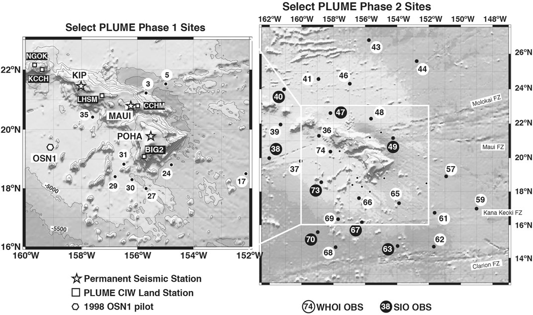
FIGURE 1. Site locations of the two deployment phases of the Hawaiian PLUME project. Phase 1 operated from January 2005 through January 2006 and phase 2 from April 2006 through June 2007. Only the sites discussed in this paper are shown. See Laske et al. (2009) for complete station and deployment history. The OSN1 label marks the location of the 1998 OSN pilot deployment (Dziewonski et al., 1991). Also shown are GSN observatory stations: KIP (Kipapa, Oahu) is jointly operated by GEOSCOPE and the U.S. Geological Survey (USGS). The primary instrument is a Wielandt-Streckeisen STS-1. The primary sensor at POHA (Pohakuloa, Hawaii), operated by the USGS, is a Teledyne-Geotech KS54000 borehole seismometer. MAUI was operated by GEOFON and featured a Wielandt-Streckeisen STS-2. The primary sensor at USGS-run MIDW (Midway Island, 28.22°N, 177.37°W, not shown), is a STS-2.

Such spectra are typically observed on broadband seismometers that have a corner period of 120 s or longer. But some spectra recorded on a Nanometrics Trillium T-40 (corner period 40 s) for the NoMelt experiment to the far south of Hawaii (Lin et al., 2016) and the ALBACORE experiment off-shore southern California (Reeves et al., 2015) also are of astonishing quality. Earth’s normal modes were never the initial target of any OBS deployment, nor was any other ultra-low-frequency signal. However, given the high costs of an OBS campaign, the fact that data are openly available to future investigators not involved in the campaign, and the fact that seismology is evolving to investigate ever-new signals, this paper makes the case that the investment in a high-quality seismic sensor may be a wise one, even for a free-fall OBS.

In the following sections, we first introduce general instrumentation requirements for observing Earth’s normal modes. We then elaborate on our PLUME deployments near Hawaii and place it in context with the previous OSN pilot experiment (Dziewonski et al., 1991). A detailed comparison between our OBS observations on one hand but also in the context of land installations on the other documents the consistently high quality of ultra-low frequency normal mode spectra, particularly those on Nanometrics Trillium T-240 seismometers. A note of caution hereby addresses the contamination by low-frequency transients during earlier deployments of Scripps Institution of Oceanography (SIO) instruments. We also discuss spectra collected on more recent deployments such as the NoMelt experiment (Lin et al., 2016), the ALBACORE deployment (Reeves et al., 2015) and a short test deployment off-shore southern California (Berger et al., 2016). All of these used SIO instruments but do not have the ‘transients problem’.

2 Requirements to Observe Earth’s Normal Modes: Instrumentation and Installation

2.1 Instrumentation

Of all seismic data, Earth’s free oscillations (normal modes) probably pose the highest demands on seismometry. To be recorded with high fidelity, noise levels in a seismic record have to stay consistently low for several days, sometimes weeks, without interruption or the interference from other seismic events. Normal mode seismometry therefore relies on the records of observatory instruments such as those of the GSN, GEOSCOPE (the French global network) or GEOFON (the German global network). The instruments of these permanent installations are typically located in a sheltered environment such as a vault, an abandoned mine or a borehole. A very-broadband sensor, such as a Wielandt-Streckeisen STS-1 vault seismometer or a Teledyne-Geotech KS54000 borehole seismometer, is needed to record Earth’s normal modes at frequencies below 1 mHz with high fidelity (Figure 2). The broadband Wielandt-Streckeisen STS-2 and the Güralp CMT-3T seismometers that are often used in temporary deployments or regional seismic networks are typically not considered to be in this category. However, the GEOFON and German Regional Seismic Network (GRSN) network operators achieved a remarkable noise reduction on their STS-2 installations by thermally insulating the sensor with a thermal blanket inside an aluminum bell jar (Hanka, 2000). This noise reduction consistently allows the observation of low-frequency normal modes after large earthquakes down to mode ${{\displaystyle {}_{0}S}}_4$ (0.647 mHz).

FIGURE 2

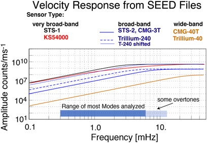
FIGURE 2. Long-period protion of the velocity response of sensors used in broadband seismology. The Wielandt Streckeisen STS-1 vault seismometer (corner period 360 s) and the Teledyne-Geotech KS54000 borehole seismometer are considered very broadband sensors, while the STS-2 and the Güralp CMG-3T (corner period 120 s) are broadband sensors. The Nanometrics Trillium T-240 (corner period 240 s) falls in between. Sensors with a corner period of 40 s (e.g. the Trillium T-40 or the CMG-40T) are wideband sensors (often mislabelled as broadband). For better comparison of the low-frequency roll-off of the Trillium 240 with that of the STS-1, it is also plotted with a thin blue line and shifted to match the STS-1 response at 10 mHz.

Ocean islands are usually thought of as being noisy sites for the GSN. In the microseism band between 15 and 5 s, noise levels can easily be 10–20 dB higher than at stations in the interiors of continents. On the other hand, and somewhat curiously, several Pacific island sites are some of the world’s quietest to record vertical ground motion in the free oscillation band at periods longer than 200 s (frequencies below 5 mHz). This includes station KIP (Kipapa, on Oahu; Hawaii) but also GEOSCOPE stationPPT (Pamatai, Papete; Tahiti). Supplementary Figure S1 shows some examples of noise curves published in the Federation of Digital Seismic Network (FDSN) station book. Station KIP compares favorably to remote installations in the interiors of continents even for the horizontal components. In this paper, we concentrate our discussion on vertical components, for two reasons. The vertical components are usually the quieter components in general. Secondly, the normal mode spectra of vertical components are easier to assess because of the general absence of toroidal modes as they have only horizontal motion, and so spectral peaks are farther apart on the vertical component than on the horizontal components that record both spheroidal and toroidal modes.

2.2 Benchmark Earthquake–The 1998 Balleny Island Earthquake at Ocean Seismic Network1

On the ocean floor, long-period noise levels are reported to be considerably higher than on land as a consequence of exposure to wind-generated infragravity waves (Webb, 1998). It has therefore been expected that free oscillations can only be observed on buried sensors. Even then, burial does not guarantee success. For example, the buried and cabled ocean bottom station H2O, halfway between Hawaii and the coast of Oregon was operational between 1999 and 2003 and was witness to several large earthquakes. But we did not obtain any convincing and consistent normal mode spectrum. The exact sensor type was a subject of long debate but may not have been a broadband sensor after all.

Just before H2O went online, the Ocean Seismic Network (OSN) initiative deployed a KS54000 very-broadband borehole sensor at ODP site 843B south of Oahu, Hawaii, about 250 m below the seafloor (Dziewonski et al., 1991; Vernon et al., 1998). During this roughly 4-months long pilot deployment, OSN1, the great $M_S=8.0;M_0=17.0\times {10}^{20}$ Nm Balleny Island earthquake occurred on March 25, 1998. This event was perhaps the first great earthquake for which free oscillations were observed on the ocean floor (Figure 3), and we use it as benchmark for normal mode observations during the later PLUME deployments.

FIGURE 3

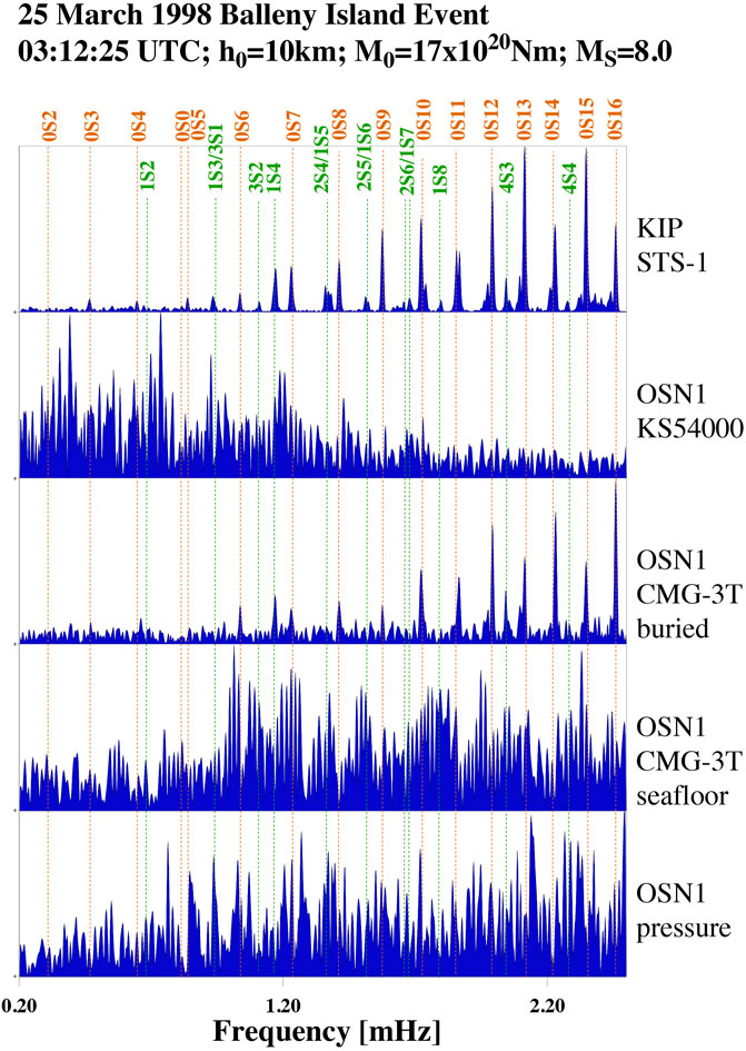
FIGURE 3. Raw vertical-component spectra for the March 25, 1998 Balleny Island earthquake of 50-hour long segments, starting 1.5 h after the source time. Hanning tapers are applied. Shown are spectra for GSN station KIP and the ocean bottom sensors deployed at OSN1(Figure 1). Comments below the station name denote the seismic sensor. At OSN1, pressure was recorded on a Cox-Webb differential pressure gauge (DPG Cox et al., 1984). In the frequency range shown here, corrections for respective instrument responses (Figure 2) change the relative shape of the spectra only marginally, but modes and background noise at frequencies below 1 mHz would be enhanced. The spectra are self-normalized for optimal display. Orange lines mark fundamental mode frequencies for model PREM(Dziewonski and Anderson, 1981), while green lines mark overtones.

To keep the data processing consistent between deployments and between earthquakes, we perform minimal data editing which may include the interactive removal of single-point spikes or similar. We apply bandpass convolution filters with a 40-dB lowpass roll-off between 40 and 50 mHz and a gently decaying highpass with a roll-off of 20 dB between 0 and 0.5 mHz to suppress tidal signals. A Hanning taper is applied before computing the spectra. But we do not correct for the instrument response, nor do we perform any noise-optimization measures such as the correction for tilt and/or pressure (Webb and Crawford, 1999; Crawford and Webb, 2000; Bell et al., 2015).

At stations on land, normal modes can be observed very clearly down to mode ${{\displaystyle {}_{0}S}}_3$ (0.469 mHz) at the quietest GSN stations, including KIP (Figure 3). No other station nearby was available or recorded this event with high fidelity. Not shown, Rayleigh wave train $R_1$ is discernible in the STS-2 record at XMAS (Kiritimati Island, Kiribati), about 2,600 km from Hawaii, but significant long-period noise does not allow us to identify any modes. Station JOHN (Johnston Atoll, operated by the USGS) started operation not until July 1998 and other stations started even later: MAUI in June 1999, POHA (Pohakuloa, Hawaii) in November 1999 and MIDW (Midway Island) in June 2002.

At OSN1, the spectrum for the KS54000 fails to show Earth’s normal modes. Unfortunately, long-period convection of fluids in the borehole caused long-period noise (Vernon et al., 1998) to levels too high for standard normal-mode observations that involve time series lengths of several days. For extremely short windows (e.g. 20 h), some isolated modes such as ${{\displaystyle {}_{0}S}}_{30}$ at 3.815 mHz appear to emerge barely above the background noise, but frequency measurements are not very robust, and the fact that neighboring modes do not appear makes these observations suspect. OSN1 also operated two broadband OBSs (BBOBSs). One was placed on the seafloor, while the other one was buried about half a meter using a remotely operated vehicle (ROV) (Collins et al., 2001). The buried CMG-3T had noise levels low enough for clear normal mode observations down to mode ${{\displaystyle {}_{0}S}}_6$ (1.038 mHz) (Figure 3). However, the overall noise level was significantly higher than at KIP which hampers the identification of some overtones between the fundamental modes at frequencies near or below 2 mHz, such as modes ${{\displaystyle {}_{4}S}}_4$ and ${{\displaystyle {}_{1}S}}_8$. Neither the seafloor BBOBS nor its pressure sensor (a Cox-Webb differential pressure gauge, DPG; Cox et al., 1984) produced a consistent normal-mode spectrum. While some spectral lines for both may coincide with mode identifiers (e.g. $\frac{{{\displaystyle {}_{1}S}}_3}{S_1}$, ${{\displaystyle {}_{0}S}}_{10}$ for pressure), we very much doubt that these are actual normal mode peaks.

Events of the size of the Balleny Island earthquake occur perhaps every other year. The last previous event with a similar moment was the February 17, 1996 Irian Jaya earthquake ($M_0=24.1\times {10}^{20}$ Nm). The Balleny Island event was surpassed in moment not until the June 23, 2001 Arequipa, Peru earthquake ($M_0=46.7\times {10}^{20}$ Nm) though a smaller, tsunami-genic earthquake ($M_0=12.4\times {10}^{20}$ Nm) occurred in New Ireland on November 16, 2000. The main point here is that a year-long temporary deployment may or may not capture such a large earthquake, perhaps more often than not missing it. Smaller events occur more frequently. However, since the Balleny Island earthquake produced observable low-frequency normal modes only on the buried OBS, perhaps expectations were justifiably low for Earth’s normal modes to be observed on free-fall OBSs. This has proven too pessimistic, as the following examples will show.

3 The Hawaiian Plume-Lithosphere-Undersea-Mantle Experiment Project

In 2005, we launched a large broadband OBS network to investigate the fine-scale seismic structure of the crust and mantle beneath Hawaii (Figure 1). The PLUME OBS network included 73 sites that were occupied in two phases by 74 instruments (Laske et al., 2009). These instruments were provided by the two OBSIP institutional operators at the time: SIO and Woods Hole Oceanographic Institution (WHOI). The Carnegie Institution of Washington (CIW) operated ten temporary land stations for the entire duration of the field campaign. An inner OBS network of 35 sites recorded continuously from January 2005 through January 2006 (phase 1). An outer OBS network of 38 sites recorded from April 2006 through June 2007 (phase 2). During both deployment phases, the WHOI instruments were equipped with Güralp CMG-3T sensors. PLUME was the first experiment to deploy these OBSs in large numbers. The SIO instruments featured a Nanometrics Trillium T-40 wideband sensor during phase 1 and a Trillium T-240 broadband sensor during phase 2. All instruments included a Cox-Webb DPG (Cox et al., 1984). Several instruments were lost, some instruments did not record useful seismic signal, and some sites were excluded for other reasons (e.g., some phase 1 SIO OBSs recorded only on horizontal components). Figure 1 shows only the sites discussed in this paper.

During the two PLUME OBS deployments, 11 great earthquakes with scalar seismic moments $M_0=2.0\times {10}^{20}$ Nm or larger occurred (Supplementary Table S1) each of which excited Earth’s free oscillations. Five of these events had a scalar seismic moment similar or larger than the 1998 Balleny Island event, with one of them during phase 1. With a scalar seismic moment $M_0=111\times {10}^{20}$ Nm, the great March 28, 2005 Sumatra-Andaman earthquake, was by far the largest earthquake. Accordingly, normal modes can be observed to frequencies far below 1 mHz, even on the OBSs (Figure 4). But our collection also includes spectra for a much smaller event. The June 13, 2005 Tarapaqa, Chile earthquake had a scalar seismic moment $M_0=5.14\times {10}^{20}$ Nm and was more than three times smaller than the 1998 Balleny Island event.

FIGURE 4

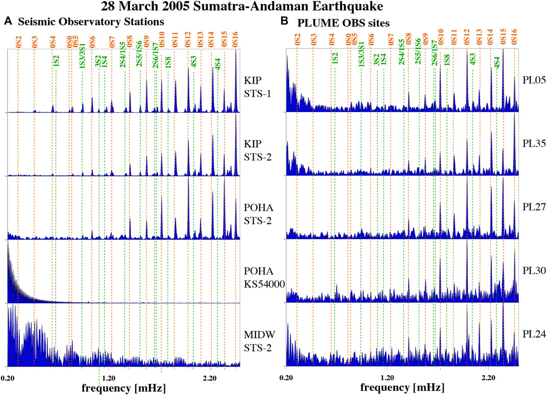
FIGURE 4. Normalized raw vertical-component spectra for the March 28, 2005 Sumatra-Andaman earthquake of 50-hour long segments, starting 1.5 h after the event time. (A) Spectra at stations of permanent observatory stations KIP, POHA and MIDW. The sensor type is listed below the stations name. Stations KIP and POHA featured two sensors, where the secondary sensor (location code 10) was a STS-2 broadband sensor. (B) Spectra at five OBS sites with the best signal-to-noise ratio. The sensor was a Güralp CMG-3T sensor. See Supplementary Table S1 in the supplement for earthquake parameters.

During the phase 2 deployment, four of the recorded events were very large, with scalar seismic moments greater than $10\times {10}^{20}$ Nm. The largest was the tsunami-genic Kuril Islands earthquake on November 15, 2006. On the vertical components, the signal-to-noise ratio (SNR) observed in the normal mode band below 10 mHz is surprisingly high on the PLUME OBSs (Laske et al., 2007). In fact, for the 2006 Kuril Islands event, it is clearly higher than on those of the PLUME land stations though not as high as on those of observatory stations KIP, POHA and MIDW.

3.1 The March 28, 2005 Sumatra Earthquake

The March 28, 2005 Sumatra earthquake was an aftershock of the devastating, tsunami-genic December 26, 2004 Sumatra-Andaman earthquake. With a scalar seismic moment $M_0=111\times {10}^{20}$ Nm, this event was 6.5 times larger than the 1998 Balleny Island event. We therefore hoped that SNRs may be high enough to observe normal modes on unburied seismometers. At land station KIP, the free oscillation spectrum is of extremely high quality (Figure 4A). Mode ${{\displaystyle {}_{0}S}}_3$ (0.469 mHz) that is observed only for the largest earthquakes can be identify clearly (in the STS-1 record) and several other very quiet GSN stations. AT KIP, even the STS-2 record has SNRs high enough to observe mode ${{\displaystyle {}_{0}S}}_4$ (0.647 mHz). The KS5400 at POHA did not record any seismic signals at the time, so no modes can be seen in the spectrum. At frequencies below 2 mHz, the STS-2 record at this location is significantly noisier than that at KIP but mode pair $\frac{{{\displaystyle {}_{1}S}}_3}{S_1}$ at 0.94 mHz may rise above the noise. At station MIDW, the first four surface wave trains can be observed during the first 6 h after the event before the records are severely contaminated by secondary signals. This is too short to make any meaningful mode measurements.

The quality of spectra recorded on the PLUME OBSs varies greatly, but mode ${{\displaystyle {}_{0}S}}_8$ (1.412 mHz) clearly stands out against the background noise, and at some sites we may even observe mode ${{\displaystyle {}_{0}S}}_6$ (1.038 mHz) (e.g. PL35 in Figure 4B). The figure shows the best five spectra but there are several others of nearly the same quality. Noise levels in these spectra are higher than those of the STS-2 at land station POHA. However, compared to the 1998 Balleny Islands spectrum of the unburied BBOBS at OSN1, we are not only able to identify normal modes in the PLUME OBS spectra, but also to very low frequencies below 1.5 mHz. To our knowledge, these are the first ever mode observations on OBSs at such low frequencies. Inspection of the DPG records is discouraging as we cannot consistently identify large groups of modes in any of the spectra.

3.2 The June 13, 2005 Tarapaca, Northern Chile Earthquake

Events as large as the March 28, 2005 Sumatra event occur perhaps less than once a decade. High-quality spectra for this event therefore should be expected, and a favorable comparison with the 1998 Balleny Island may not be representative of the high quality of spectra collected for the PLUME project. We therefore also inspect smaller events. Figure 5 shows the spectra of the $M_S=7.9;M_0=5.14\times {10}^{20}$ Nm June 13, 2005 Tarapaca, Northern Chile earthquake that was more than 3 times smaller than the 1998 Balleny Island event. This earthquake was followed about 28 h later by a $M_S=7.0$ event in the Gorda Plate off the coast of California. Even though the scalar seismic moment was less that $1\times {10}^{20}$ Nm, this event produced waveforms at Hawaiian stations so that spectra for the Tarapaca event have to be calculated for shorter time windows, and we would normally not include this event in our normal mode analyses. But to prove the point of observability, the STS-1 spectrum at KIP clearly shows mode ${{\displaystyle {}_{0}S}}_5$ (0.840 mHz) against the background noise. Robust measurements may also be possible for mode ${{\displaystyle {}_{0}S}}_4$ (0.649 mHz). The STS-2 spectrum as well as the spectra at POHA show modes down to ${{\displaystyle {}_{0}S}}_6$ (1.038 mHz), while modes down to ${{\displaystyle {}_{0}S}}_8$ (1.413 mHz) can be discerned at station MIDW. The spectra at the PLUME OBSs are considerably noisier but some instruments clearly show mode ${{\displaystyle {}_{0}S}}_{13}$ (2.112 mHz) consistently against the background noise. This is in stark contrast to the surface BBOBS of OSN1.

FIGURE 5

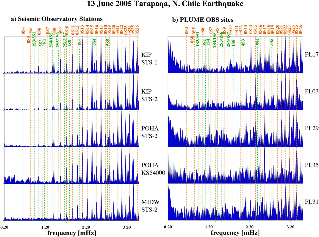
FIGURE 5. Normalized raw vertical-component spectra for the June 13, 2005 Tarapaqa, Northern Chile earthquake of 25-hour long segments, starting 1.5 h after the event time. (A) Spectra at stations of the GSN; (B) Spectra at five OBS sites with the best signal-to-noise ratio. See Supplementary Table S1 in the supplement for earthquake parameters. This event was more than three times smaller than the 1998 Balleny Island earthquake (see Figure 3). Yet, we are able to observe normal modes on unburied OBSs.

3.3 The November 15, 2006 Kuril Islands Earthquake

During PLUME phase 2, we captured four very large earthquakes with scalar seismic moment $M_0=10\times {10}^{20}$ Nm or larger. The events occurred in different source regions so were not associated with the great December 26, 2004 Sumatra-Andaman earthquake.

With a scalar seismic moment $M_0=35\times {10}^{20}$ Nm, the November 15, 2006 Kuril Islands event was the largest of the phase 2 events. Figure 6 shows the spectra at the GSN and PLUME land stations. For this event, the record at KIP is somewhat noisier than that at the other GSN stations. At POHA and perhaps at MIDW, mode ${{\displaystyle {}_{0}S}}_5$ (0.840 mHz) rises above the background noise, while the first robust observation at KIP is probably that of mode ${{\displaystyle {}_{0}S}}_6$ (1.038 mHz). For such a large earthquake, and to analyze the lowest-frequency modes, we would choose a longer time window. For example, the time in which the amplitude of mode ${{\displaystyle {}_{0}S}}_4$ decays to $1/e$ is 98 h, so we would choose 98 h for this particular mode. In this case, only the very best GSN stations would be included in an analysis as the spectra at many stations degrade due to increasing noise contamination. However, for a consistent comparison for this paper, we keep the 50-hour windows fixed for all earthquakes shown here.

FIGURE 6

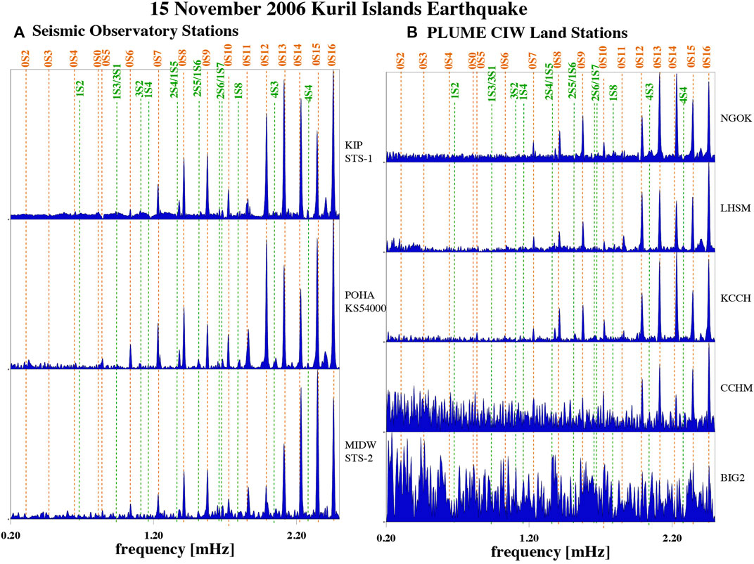
FIGURE 6. Normalized raw vertical-component spectra for the November 15, 2006 Kuril Islands earthquake of 50-hour long segments, starting 1.5 h after the event time. (A) Spectra at stations of the GSN. See Supplementary Table S1 in the supplement for earthquake parameters. (B) Spectra at the five CIW land stations still operating at the time. All CIW stations were equipped with a Wielandt-Streckeisen STS-2 seismometer.

Except for station KCCH, the noise level at the PLUME land stations is considerably higher though robust observations for mode ${{\displaystyle {}_{0}S}}_7$ (1.231 mHZ) are possible. Station KCCH may even show mode ${{\displaystyle {}_{0}S}}_5$. Among the PLUME land stations, KCCH has a vastly better spectrum than BIG2. Through a grading scheme we make a first attempt to quantify the quality of these spectra. When initially inspecting very low-frequency free oscillation spectra, we assess the overall signal-to-noise ratio over a frequency band that includes all modes up the 2 mHz, and assign grades. This will help later when zooming in on individual modes to decide whether a spectral peak is really a mode or likely noise that happens to have a frequency close to a mode frequency. Grade “A” is assigned for the best spectra for a particular earthquake. Greater earthquakes are expected to reach higher overall SNRs than smaller earthquakes, so exactly what constitutes grade “A” may vary by earthquake. For the Kuril Islands event, modes ${{\displaystyle {}_{0}S}}_6$ through ${{\displaystyle {}_{0}S}}_8$ should very clearly rise above the background noise. Grade “B” is assigned if some noise is obvious, grade “C” when modes at slightly higher frequencies (such as ${{\displaystyle {}_{0}S}}_{10}$ at 1.725 mHz) are questionable. For grade “D” modes below 2 mHz are usually not visible and grade “E” is assigned if no mode is visible in the current window but in significantly shorter ones, or if Rayleigh waves are clearly visible in the time series. Grade “F” is assigned if no seismic signal is discernible. The spectra at POHA, MIDW and KCCH are grade “A” (see also Supplementary Table S2), while that of KIP and LHSM are borderline “A” or “B”, CCHM is a “C”, while BIG2 needs extremely short windows for modes to rise above the noise (grade “E”).

Taking these spectra as benchmark, we also grade the OBS spectra (Supplementary Table S2). Spectra at some of the WHOI OBSs compare quite favorably (Figure 7). At stations PL44 and PL69 (grade “A” though PL69 experienced minor data dropouts), mode ${{\displaystyle {}_{0}S}}_6$ (1.038 mHz) rises above the noise. Regarding SNR, these spectra may be superior to the OBS spectra collected for the March 2005 Sumatra event (Figure 4) which was 3.5 times larger. The other shown WHOI spectra are grade “B”, with ${{\displaystyle {}_{0}S}}_8$ (1.413 mHz) clearly visible in most of them. The spectra at all but the prematurely failing SIO OBS site PL38 are of exceptionally high quality, with low noise levels between modes, and ${{\displaystyle {}_{0}S}}_6$ (1.038 mHz) rising above the noise very clearly in most of the spectra. All of them are grade “A” and compare favorably with the spectrum at WHOI site PL44. In fact, these spectra appear to be superior to the spectra at all PLUME land stations as Supplementary Table S2 documents.

FIGURE 7

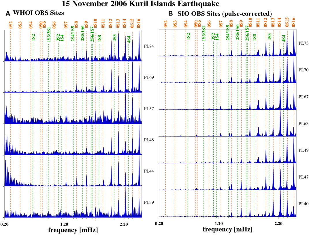
FIGURE 7. Normalized raw vertical-component spectra for the November 15, 2006 Kuril Islands earthquake of 50-hour long segments, starting 1.5 h after the event time. (A) Spectra at the six best WHOI OBS sites. The recording sensor was a CMG-3T. (B) Spectra at seven of the eight SIO OBS sites. The 8th instrument failed earlier and did not record seismic data at the time. The recording sensor was a T-240. For event details see Figure 6. The SIO spectra have been corrected for instrument-generated harmonic signals (see text for detail).

The process of assigning grades is somewhat subjective so we conduct a more quantitative assessment where we measure the peak amplitudes of the five fundamental modes ${{\displaystyle {}_{0}S}}_6$ through ${{\displaystyle {}_{0}S}}_{10}$ against the background noise using our interactive screen tool. To assess overall performance of each instrument type (SIO/WHOI OBS, CIW-land), we determine the average SNR and the standard deviation thereof for each mode (Figure 8). Analysis for several modes is necessary for a better overall assessment as small changes in location may significantly lower the SNR for a certain mode while others are not affected. The set of SNRs for the SIO instruments compare favorably with those of the PLUME land instruments (CIW), particularly for mode ${{\displaystyle {}_{0}S}}_6$. However, on average and individually, the quality does not quite reach that of station POHA (note that GSN stations KIP and MIDW also do not quite reach POHA, as discussed above). The set of WHOI OBSs fare significantly worse, with lower SNRs for all modes. The systematically smaller SNRs may be a result of the significantly larger set of stations including noisier ones. We therefore redo an analysis using only the seven best instruments. But even then, the average SNRs do not reach that of the SIO instruments nor the PLUME land stations. Together with visual inspection of the spectra, we conclude that the SIO OBSs systematically deliver higher-quality spectra for modes at the lowest frequencies.

FIGURE 8

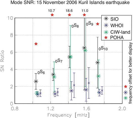
FIGURE 8. Average of signal-to-noise ratios for different instrument types and five low-frequency normal modes. Averages were determined over 7 SIO, 5 CIW-land and 17 WHOI instruments. The results are slightly offset in frequency between instrument types for better display. For reference, red stars mark the SNR measured at GSN station POHA. Blue ‘x’ mark a reanalysis of the seven best WHOI instruments.

Drawing from longtime experience with analyzing GSN data, we are aware that Güralp CMG-3T spectra can be of high quality. But the variance in the quality of CMG-3T spectra is much greater than in those for Nanometrics Trillium T-240 sensors that consistently deliver high SNR spectra. Another factor that distinguishes the two types of OBSs is the installation of the sensor: the WHOI sensor ball in which the seismometer is housed is dropped directly into the seafloor mud, while the SIO sensor ball stands on a small tripod whose footprint reaches just beyond that of the sensor ball. It has been argued that such an installation increases turbulences and may induce high-frequency noise but in-situ test deployments have so far been inconclusive (Jeff Babcock, 2016, personal communication). The tripod may well provide a more stable coupling to the ground though at this point this is highly speculative.

Unfortunately, the SIO spectra are fraught with instrument-generated low-frequency harmonic noise that remains visible even after a correction for it (see also Ringler et al., 2021). The transients were generated by the gimbal electronics in the sensor ball that awaken to check whether the seismometer needs to be relevelled. This process is a low-frequency process and is not visible in the raw data. But in lowpass filtered data, long-duration transients (up to 20 min long) become visible that have been described as ‘glitches’ (Deen et al., 2017). In the early deployments of SIO OBSs, the relevel checks were performed nearly every hour (every 3,620.56 s to be more precise) which causes the harmonics in the spectrum. Why the relevel check occurs every 3,620.56 s and not every 3,600 s is unclear. The lowest-frequency harmonic related to these checks is at 0.2762 mHz (hence the derived repeat time just mentioned). Unfortunately, higher harmonics overlap in frequency with some of Earth’s normal modes, including ${{\displaystyle {}_{0}S}}_5$ and ${{\displaystyle {}_{3}S}}_2$, which renders the spectra questionable for a mode analysis. Even at higher frequencies beyond 2 mHz, the spectral amplitude of the harmonics is quite high. Since the number of Earth’s normal modes in any given frequency interval increases with frequency, the chances increase that a higher harmonic will overlaps with a normal mode.

The transients are different in shape between different instruments (Figure 9) but are rather reproducible on the same instrument, at least within a five-day period. The temporal distance between transients also is the same between instruments. Our somewhat ad-hoc approach to remove the transients is as follows: we determine the average ‘transient’ starting 10 h into a 110-hour long time series after the earthquake. A step in the data preprocessing is a downsampling from an original sampling rate of 31.25 Hz to a sampling interval of 9.92 s. Hence our repeat transient segment is 365 samples long (3,620.8 s). We then subtract a reconstructed time series consisting of repeats of the 365-sample transient from the entire time series. Spectra before and after the correction are juxtaposed in Supplementary Figure S2. The choice to start the averaging 10 h into the time series is the results of visually optimizing the removal of the offending harmonics at ultra-low frequencies. Starting later provides a smoother average transient in the time domain and removes more of the higher harmonics beyond 5 mHz. But this leaves more harmonics at frequencies below 2 mHz. An earlier start brings no improvement. This optimal start time of 10 h after the source time may depend on the earthquake analyzed. A mismatch between the 365-sample repeat (as constrained by the 9.92 s sampling interval) and the inferred 3,620.56 s repeat from the lowest-frequency harmonic produces a one-sample (12 s) mismatch 50 h into the time series. However, a correction in a 0.992 s downsampled time series yields no noticeably improvement. Since the correction for the transients still leaves considerable signal in the spectra, we would rather not include such spectra in a normal-mode analysis, for affected modes. After providing feedback to the SIO OBS operator, the schedule for the relevel checks was changed to occur less frequently, most recently to once a week (Martin Rapa, personal communication). The examples shown in the rest of this paper are from a time after this change in protocol occurred.

FIGURE 9

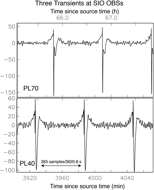
FIGURE 9. A sequence of three low-frequency transients in the bandpass filtered time series of the vertical component of SIO OBSs PL40 and PL70 many hours after the November 15, 2006 Kuril Islands earthquake. Spectral analysis indicates that the distance between pulses is 3,620.56 s, which is about 365 samples (a sample is 9.92 s, so 365 samples would be 3,620.8 s; see text for details).

4 Other Ocean Bottom Seismometer Instrument Pool Deployments in the Pacific Ocean

4.1 NoMelt

The NoMelt experiment (Lin et al., 2016; Russell et al., 2019) combined passive broadband and active-source seismic refraction/reflection surveys with the deployment of marine magnetotelluric instruments to explore 70-million year old oceanic lithosphere about 1700 km southeast of Hawaii (Figure 10). The broadband passive deployment recorded data between December 2011 and January 2013 and encompassed 20 broadband sensors as well as two additional T-40 wideband sensors. During the deployment time, six earthquakes occurred with a scalar seismic moment $M_0\ge 2.0\times {10}^{20}$ Nm (Supplementary Table S1). A seventh very large event occurred about an hour after the 11 April main shock in the Indian ocean. With $M_0\ge 29\times {10}^{20}$ Nm, this aftershock alone would probably qualify as a once-every-few-years event. The main shock was just above three times larger which makes a standard single-spectrum analysis of this event difficult unless we apply a technique such as our autoregressive splitting matrix analysis (Masters et al., 2000) that does not depend on details of the seismic source. One difficulty of analyzing spectra of such ‘double-events’ is that spectral peaks may split, thereby falsely suggesting that normal-modes splitting due to Earth structure is observed. However, for the sake of this paper, we can still explore the quality of the spectra. Of the 22 stations, seven produced grade E or F spectra and so are excluded. The remaining 15 spectra are shown in Figure 11. Because of the aftershock, we start the time window for the spectra 2 h after the source time. Since this event was so large, we increase the time window length to 60 h.

FIGURE 10

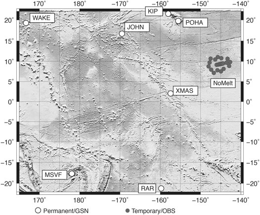
FIGURE 10. Site locations of the broadband NoMelt OBS network (Dec 2011–Jan 2013). Also shown are sites of permanent observatory stations of the GSN: KIP (Kipapa, Oahu; primary sensor: STS-1), POHA (Pohakuloa, Hawaii; KS54000), JOHN (Johnston Island; KS54000), WAKE (Wake Island; KS54000), XMAS (Kiritimati Island, Kiribati; STS-2); RAR (Rarotonga, Cook Islands (KS54000); MSVF (Monasavu, Fiji; KS54000).

FIGURE 11

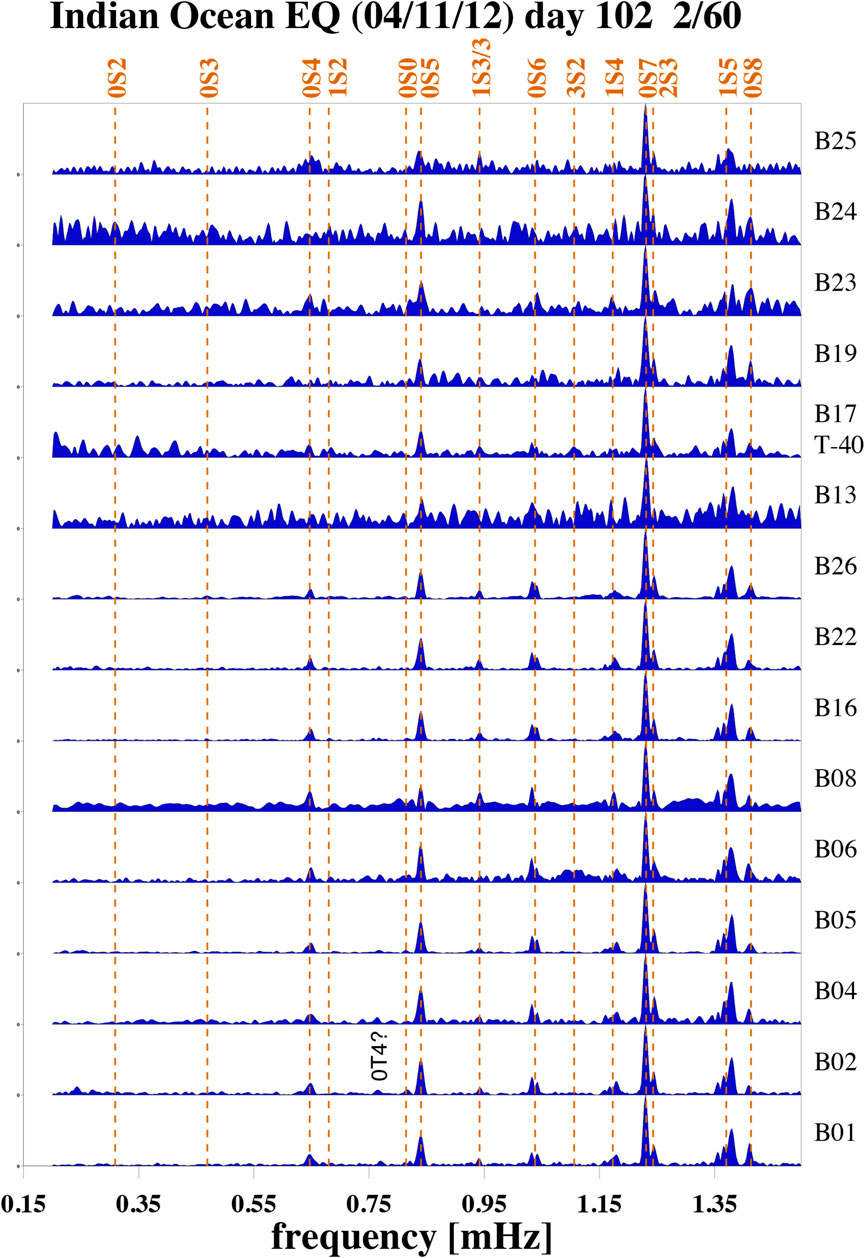
FIGURE 11. Normalized raw vertical-component spectra for the April 11, 2012 Indian Ocean earthquake of 60-hour long segments, starting 2 h after the event time. See Supplementary Table S1 in the supplement for earthquake parameters. Site B17 featured a Nanometrics Trillium T-40 wideband sensor.

A direct quantitative comparison with land installations is somewhat hampered as the closest GSN station, XMAS (Kirimati Island, Kiribati), is about 1,500 km away. At such distances, spectral amplitudes for a mode can be vastly different between stations while that of other modes are not affected as much. In a somewhat extreme case, for a station about 90° away from the source, every other fundamental mode may experience a greatly reduced amplitude (Laske and Widmer-Schnidrig, 2015). Bearing this in mind, Figure 12 displays seven representative spectra in the southwestern Pacific ocean. For all but one station (MSVF) we consider both the primary and the secondary sensors (location codes 00 and 10) and make a decision which sensor in the better one to include in this study. For stations WAKE, RAR and XMAS, we choose the secondary sensor, a Wielandt-Streckeisen STS-2. At XMAS, the record of the primary sensor was a grade F, at WAKE we see a Rayleigh wave on the primary sensor but normal mode peaks appear only at frequencies above 2 mHz and only if we take shorter records (grade E). At station RAR, the quality of the spectrum for the primary sensor was of marginally less quality than that of the secondary sensor though it would hamper analysis of mode ${{\displaystyle {}_{0}S}}_3$ (0.469 mHz).

FIGURE 12

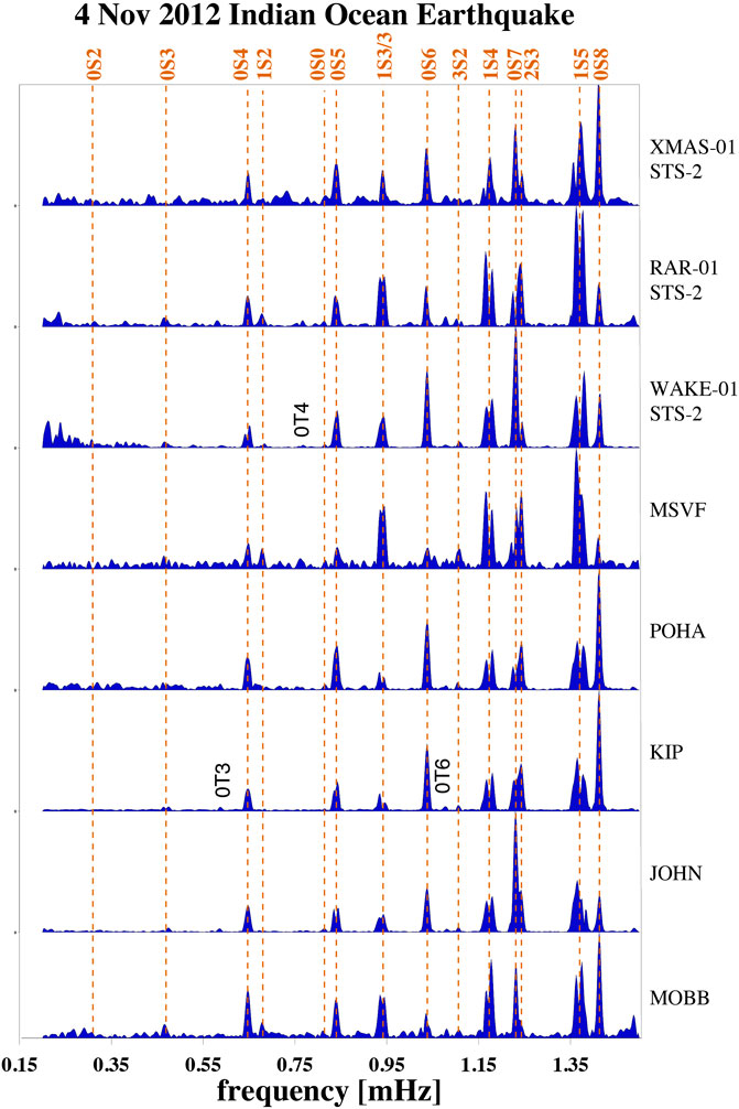
FIGURE 12. Normalized raw vertical-component spectra at GSN stations for the April 11, 2012 Indian Ocean earthquake of 60-hour long segments, starting 2 h after the event time. A code 01 after the station code means that we use the secondary sensor for analysis (sensor type below the station name). Also shown is the spectrum of seafloor observatory MOBB off-shore California (see Figure 13).

The spectra for this event are remarkable, for a number of reasons. Firstly, mode ${{\displaystyle {}_{0}S}}_3$ clearly appears above the background noise at a number of GSN stations and may be observed at even the one or other NoMelt OBS (e.g., B26). Together with mode ${{\displaystyle {}_{0}S}}_2$ (0.309 mHz), this mode is rather rarely observed, and only on records of the highest GSN quality. Secondly, mode ${{\displaystyle {}_{0}S}}_4$ (0.647 mHz) appears clearly against the background noise at about half of the NoMelt OBS sites, a document of perhaps the best-quality OBS normal mode spectra on OBSIP OBSs collected so far. Thirdly, one of these spectra is that of station B17. According to the meta data, this site was equipped with a wideband sensor (T-40). There always is a possibility of an error in the meta database. However, inspection of the spectra confirms that this was a T-40. Evaluating the instrument responses in Figure 2, a raw signal at 1 mHz is likely reduced by a factor of about 20 when compared to a signal at 40 mHz. In our raw spectra, the low-frequency roll-off is much steeper at this site than at the other sites (Supplementary Figure S3). Arguably, the B17 spectrum in Figure 11 is the noisiest of the ‘good’ spectra but the fact that this instrument recorded low frequency modes at such high quality, let alone having mode ${{\displaystyle {}_{0}S}}_5$ stand out clearly above the background noise is a manifest for exceptional low-frequency performance of this particular sensor. Unfortunately, we are unable to backtrack the physical specifications (i.e. serial numbers) of the OBS hardware, including the sensor as the packages are routinely taken apart and reassembled for future deployments. But we note that the ALBACORE deployment in the California Borderland (see next section) also had such an exceptional T-40 performance.

To complement the comparison, seafloor observatory MOBB off-shore California (Romanowicz et al., 2006) (Figure 13) also recorded this event with high fidelity. This site has a broadband Güralp CMG-1T seismometer that is buried beneath at least 10 cm of sediments and is located at a water depth of 1,000 m. At this water depth, we normally expect high noise levels in the infragravity band at frequencies below about 10 mHz. Yet, the spectrum at MOBB is also of extremely high quality where mode ${{\displaystyle {}_{0}S}}_4$ easily stands out against the background noise, and even mode ${{\displaystyle {}_{0}S}}_3$ is clearly discernible. A SNR analysis similar to that in Figure 8 can be found in the online supplement (Supplementary Figure S4). Mode ${{\displaystyle {}_{0}S}}_6$ has a relatively low SNR because the spectral amplitude of that mode is relatively low at this station. But the other modes compare favorably. In fact, mode ${{\displaystyle {}_{0}S}}_4$ has a higher SNR than the average of the GSN records considered here.

FIGURE 13

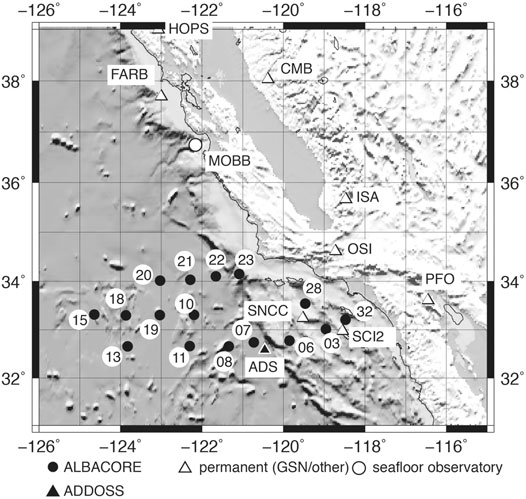
FIGURE 13. Site locations of the 16 broadband stations of the ALBACORE network (Aug 2010–Sep 2011) used in this study. Also shown are sites of permanent observatory stations of the GSN: PFO (Piñon Flat Observatory; primary sensor: STS-1), stations of the CI network (OSI, Osito Adit, STS-1; ISA, Isabella; ,STS-1; SNCC, San Nicolas Island, STS-1; SCI2, San Clemente Island, STS-2), stations of the BK network (HOPS, Hopland Field station, STS-1; CMB, Columbia College, STS-1; BKS, Berkeley, Byerly Vault, STS-1; FARB, Farallon Islands, STS-2) and seafloor observatory MOBB (Monterey Bay Broadband Ocean Botton Seismic Observatory, CMG-1T). The ADDOSS OBS as site ADS operated Dec 2013 through Mar 2014 (Berger et al., 2016). A student-led repeat deployment followed in summer 2015.

Noteworthy, a number of GSN stations but also NoMelt OBSs exhibit spectral peaks at the frequencies for toroidal modes ${{\displaystyle {}_{0}T}}_6$ (1.079 mHz), ${{\displaystyle {}_{0}T}}_4$ (0.767 mHz), and in some cases even ${{\displaystyle {}_{0}T}}_3$ (0.588 mHz). Toroidal modes have exclusively horizontal shear motion and so should show only on horizontal seismometer components. However, mode coupling between spheroidal and toroidal modes caused by the Coriolis force can cause toroidal-mode energy to appear on the vertical seismometer component. This effect is particularly strong when the frequencies of a ${{\displaystyle {}_{0}S}}_l$ mode is close to that of a ${{\displaystyle {}_{0}T}}_{l+1}$ mode (e.g. Masters et al., 1983) and is well-observed for normal modes at frequencies above 1.8 mHz. In rare cases, for very large earthquakes and exceptionally high SNR-stations, toroidal modes can be observed on vertical components in the ultra-low frequency band below 1 mHz as well (Zürn et al., 2000) as a result of Coriolis coupling and, to a lesser extent, mode coupling caused by Earth’s ellipticity and 3-dimensional structure, and even though normal mode frequencies are not as close.

We also inspect all of the NoMelt DPG spectra. While it is tempting to associate individual peaks across all stations with a normal mode, none of the 22 DPG exhibits a consistent spectrum that displays at least three adjacent fundamental modes with clear SNRs, regardless of the time series length. On the other hand, such sensors allow the analysis of semi-diurnal tidal peaks (e.g. Doran et al., 2019). Since the tidal signal is much larger than that of earthquakes, we infer that noise levels in the free oscillation band are too high to observe even very large earthquakes.

4.2 ALBACORE

The passive broadband OBS deployment for the ALBACORE experiment in the California Borderland (Reeves et al., 2015) occurred from August 2010 through September 2011 and so immediately preceded the NoMelt experiment. The metadata at the IRIS DMC includes station information for 36 OBS sites. Twelve of these were equipped with short-period instruments. Three of the remaining sites were equipped with a T-40 wideband sensor, while the rest had a T-240 broadband sensor. We obtained data for 21 stations. Five of these are grade F, exhibiting only bit noise (i.e. signals of a few counts), one T-40 record was suspicious (counts were primarily single-sided). This leaves us with usable records at 16 OBS sites (see Figure 13), one of which featured a T-40. In the following, we use four letters to name the stations though the original station names consist of five (OBS?? where ‘?’ is a number). During this deployment, four large distinct earthquakes occurred. By far the largest was the March 11, 2011 Tohoku, Japan earthquake (scalar seismic moment $M_0=531.2\times {10}^{20}$ Nm). Two large aftershocks to this earthquake occurred within 30 min which we do not consider separate free-oscillation earthquakes, and our analysis starts 2 h after the main shock. For an earthquake this large, expectations are high that even the noisiest station should produce a good SNR free oscillation spectrum.

Accordingly, spectra collected on land stations are of the highest quality and set a rather high bar for any OBS recording (Figure 14). The spectra of the best stations clearly show the gravest mode ${{\displaystyle {}_{0}S}}_2$ (0.309 mHz) rising above the noise (Supplementary Figure S6 in the supplement provides a zoom-in). These include stations PFO, CMB and HOPS, and perhaps OSI and even SNCC. On the other hand, stations SCI2 and ISA (not shown) have rather noisy spectra where mode ${{\displaystyle {}_{0}S}}_6$ is probably the lowest-frequency mode above the noise. Also shown in the figure are spectra at six of the ALBACORE sites. At least five more OBS spectra have this kind of quality (Supplementary Figure S5). While we should not hope to observe the gravest modes at frequencies below 0.5 mHz (many GSN stations do not rise to this bar), modes ${{\displaystyle {}_{0}S}}_5$ (0.840 mHz), ${{\displaystyle {}_{0}S}}_0$ (0.814 mHz) and ${{\displaystyle {}_{0}S}}_4$ (0.647 mHz) clearly rises above the noise, and maybe even ${{\displaystyle {}_{0}S}}_3$ (0.469 mHz). These observations should make the ALBACORE and the NoMelt experiments the first broadband OBS experiments that allowed free oscillation observations to such low frequencies.

FIGURE 14

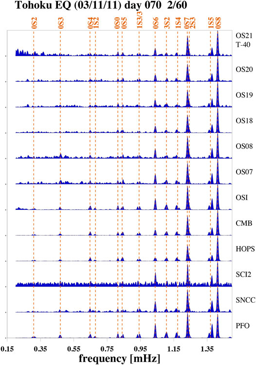
FIGURE 14. Normalized raw vertical-component spectra for the March 11, 2011 Tohoku, Japan earthquake of 60-hour long segments, starting 2 h after the event time. The bottom six spectra are from permanent land stations (see 15), while the top six spectra are for ALBACORE OBS sites. Site OS21 featured a Nanometrics Trillium T-40 wideband sensor. See online supplement for the spectra of all broadband OBSs.

Most remarkably, the sensor at site OS21 is the wideband T-40. A double-check of the raw spectra confirms a similar finding as that of site B17 for NoMelt and confirms that we are dealing with a T-40 and not a typo in the metadata. At this point, we doubt that all T-40s perform this well but as described above, the other two T-40s in this experiments did not provide usable data. One must wonder whether this was the same sensor as that at NoMelt site B17. Unfortunately, this sensor is likely no longer in the fleet as the SIO OBS group subsequently exchanged T-40 sensors for T-240s. While T-240s are expected to perform better in the free oscillation band, the loss of this particular T-40 is arguable a great loss for ocean bottom normal-mode seismology and engineering alike. It would have been nice to explore in more detail exactly what made this particular sensor so unique in its performance.

The deployment of ALBACORE OBSs in a wide range of water depths allows us to explore the influence of water depth on the quality of the free-oscillation SNR. While most of the OBSs were deployed in the deeper ocean at depths greater than 3,500 m, even the spectrum for OS23 at a water depth near 2000 m is acceptable (see Supplementary Figure S5). But a deployment at shallower depths clearly increases noise levels. To quantify this further, we measure the SNR for six modes at the six shallowest sites and compare that against the SNR at the other ten sites. A split into four shallow vs twelve deeper sites would follow the narrative above better, but we feel that the subsequently smaller standard deviations for smaller samples would not be representative. Figure 15 confirms that the shallower sites have lower SNRs for all modes than the deeper sites. The relatively low SNR for mode ${{\displaystyle {}_{0}S}}_9$ is a result of relatively low spectral amplitudes at some OBSs, compared to neighboring modes, or even neighboring OBSs. For comparison, we also determine the SNR for a set of ten spectra at nine land stations: SNCC, SCI2, PFO, OSI, ISA, BKS, CMB, FARB and HOPS. As expected, SNRs at permanent observatory seismic stations are consistently higher than those at the OBS sites. Spectral amplitudes for mode ${{\displaystyle {}_{0}S}}_9$ are relatively low at northern California stations, which results in lower SNRs at the land stations as well.

FIGURE 15

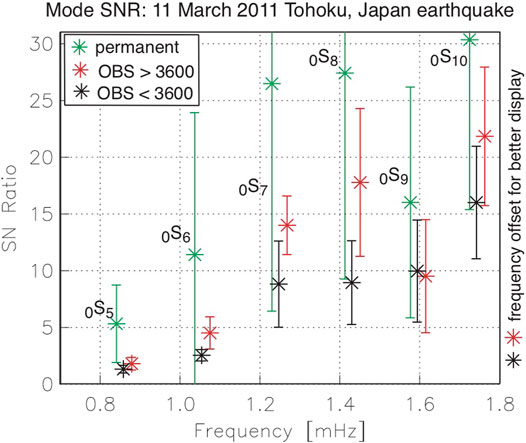
FIGURE 15. Average of signal-to-noise ratios for the 16 ALBACORE stations that had useful seismic data (15 broadband, 1 wideband). The results are slightly offset in frequency between instrument types for better display. Six grade-E or F stations were discarded and not included (5 broadband, 1 wideband). Black: 10 OBSs in deeper water ($>$3,600 m). Red: 6 OBSs in shallower water ($<$ 3,600 m). Green: Average over 10 records at nine permanent land stations (shown in Figure 13).

We briefly also discuss the other large earthquakes observed at the ALBACORE deployment. With a scalar seismic moment $M_0=2.99\times {10}^{20}$ Nm, the July 6, 2011 Kermadec earthquake is one of the smaller ones in our list. The spectra for 40-h time series exhibit normal modes with good SNR at OBSs OS13, OS11 and OS07, while spectra at OS15, OS19 and OS22 exhibit more noise though modes are still clearly visible down to mode ${{\displaystyle {}_{0}S}}_{10}$ (1.725 mHz). The seafloor depths overlap so we find no obvious relationship. The quality of spectra at the island and land stations in southern and northern California also varies. Station SNCC has an excellent spectrum that compares well with that of the best land stations, while SCI2 has a rather noisy spectrum. Station SNCC has higher SNR down to mode ${{\displaystyle {}_{0}S}}_8$ (1.413 mHz) than at the primary sensor at PFO. Mode ${{\displaystyle {}_{0}S}}_4$ (0.647 mHz) still rises above the noise. This earthquake has a record at seafloor observatory MOBB but its spectrum does not show any modes, nor do those at stations OSI and ISA that usually produce high-quality spectra.

With a scalar seismic moment $M_0=6.77\times {10}^{20}$ Nm, the October 25, 2011 Mentawai, Sumatra earthquake was more that twice as large but the spectra in California are noisier than those of the Kermadec earthquake. Station MOBB has no record for this time. On the best land station in southern California, mode ${{\displaystyle {}_{0}S}}_8$ (1.413 mHz) rises above the noise for the secondary sensor at station PFO, while stations OSI and ISA are much noisier. In northern California, mode ${{\displaystyle {}_{0}S}}_5$ (0.840 mHz) rises above the noise at stations HOPS and CMB. The best stations of the ALBACORE deployment show modes consistently above the noise down to mode ${{\displaystyle {}_{0}S}}_{15}$ (2.345 mHz), at sites OS07, OS08 and OS13 (water depths ranging from 3,769 to 4,281 m). Individual spectral peaks may align with single modes at lower frequencies though this alignment may be coincidence rather than a high-SNR mode observation.

The December 21, 2010 Izu Bonin was an earthquake with a scalar seismic moment less than $M_0=2\times {10}^{20}$ Nm. Nevertheless spectra for 40-h time series are of high quality at stations HOPS, FARB, CMB and BKS, with mode ${{\displaystyle {}_{0}S}}_7$ clearly rising above the noise (HOPS even shows ${{\displaystyle {}_{0}S}}_6$). On the other hand, spectra at other stations are rather noisy (SCI2, ISA), and the lowest-frequency mode observed at PFO is ${{\displaystyle {}_{0}S}}_{13}$ (2.112 mHz). Against this backdrop, it is perhaps remarkable, that some OBSs (OS18, OS13, OS11) exhibit normal mode spectra of better quality than at PFO, with ${{\displaystyle {}_{0}S}}_{12}$ (1.989 mHz) and all modes at higher frequencies consistently above the noise, whereby OS11 includes lower-frequency modes to maybe even ${{\displaystyle {}_{0}S}}_6$. A forth OBS (OS08) is slightly noisier. All four OBS were located at water depth greater than 3,800 m. Unfortunately, the lack of a record at seafloor observatory MOBB does not allow a comparison.

4.3 ADDOSS

Another deployment of broadband OBSs in the California Borderland was the ADDOSS (Autonomously Deployable Deep-Ocean Seismic System) experiment (Berger et al., 2016). The final of several deployments occurred from December 2013 through March 2014 on the deep-ocean side of the Patton Escarpment (site ADS3 in Figure 13) where two broadband OBSs were deployed within 1 km of each other. The primary goal of this deployment was a proof-of-concept study that a wave glider can hold station around the OBS drop location and serve as acoustic-satellite relay to transmit data from the ocean floor to a desktop computer on land in near-real time. During the three months, we recorded numerous teleseismic, regional and local earthquakes, but the scalar seismic moment of the largest earthquake remained below $M_0=0.4\times {10}^{20}$ Nm. Hence the deployment was no witness to a free oscillation earthquake.

We were luckier when one of the ADDOSS instruments was redeployed 18 months later as a piggy-back to a short student-led experiment near the ADS3 site. With a scalar seismic moment $M_0=32.3\times {10}^{20}$ Nm, the September 16, 2015 Chile earthquake was the largest earthquake for the year. This earthquake produced free oscillation spectra of the highest quality at GSN station PFO, and CI stations OSI and ISA. While the primary sensor at PFO exhibited some noise, Earth’s gravest mode ${{\displaystyle {}_{0}S}}_2$ (0.309 mHz) rises clearly above the noise floor in the spectrum of the secondary sensor (T-240) and at station OSI. On the other hand, the spectrum at island station SCI2 is extremely noise, where mode ${{\displaystyle {}_{0}S}}_9$ (1.577 mHz) barely rises above the noise, while station SNCC did not record that day. Since the spectrum at ADS3 in only marginally better than that at SCI2, we do not show a figure for this event. The stations to the north fared only marginally better. While ${{\displaystyle {}_{0}S}}_2$ also shows up in the spectra at stations BKS, CMB and HOPS, island station FARB is noisy, with perhaps ${{\displaystyle {}_{0}S}}_7$ (1.231 mHz) rising above the noise. MOBB recorded this event as well. Its background noise in much less, allowing the observation of ${{\displaystyle {}_{0}S}}_7$, and perhaps even ${{\displaystyle {}_{0}S}}_6$ (1.038 mHz). But given the discussion of previous events, the data quality on OBSs for this event is somewhat disappointing. We cannot easily explain why noise levels were so high. There was no storm activity in the area. The earthquake produced a tsunami that was still measurable at local tide gauge stations (on the order of less than 10 cm). Tsunami are recorded quite well on the horizontal OBS components (e.g., Nov 2006 Kuril Islands earthquake during PLUME), but not on the vertical. So this should not explain increased noise levels.

5 Summary and Discussion

We showed vertical-component free oscillation spectra for data collected during a number of ocean bottom seismometer (OBS) deployments in the Pacific Ocean that occurred over the last 20 years. Broadband seismology on the ocean floor using free-fall OBSs is expected to be hampered at long periods as a result of noise contamination by ocean infragravity waves. Yet, our examples showed that some spectra collected on broadband seismic sensors in the free oscillation band can reach the quality a data analyst is used from land observatory stations such as those of the Global Seismographic Network (GSN). This includes mode observations at frequencies below 1.5 mHz which require low-noise records several days long.

The SIO OBSs that are equipped with a Nanometrics Trillium T-240 sensor were found to produce consistently high-quality spectra to very low frequencies. Records include even diurnal and semi-diurnal tidal modes (e.g. Doran et al., 2019) which helps recalibrate nominal instrument responses for the pressure sensors, typically a broadband Cox-Webb differential pressure gauge (Cox et al., 1984) where sensor sensitivities can effectively vary by a factor of two. Earlier SIO OBS records are contaminated by approximately hourly transients that hamper a normal modes analysis, at least for certain modes. A removal of these signals in post-processing is moderately successful, as we and others showed (Deen et al., 2017). The low-frequency transients are generated in the electronics to check whether the seismometer needs to be relevelled even though the sensor is not mechanically relevelled. For the SIO OBSs that were part of the national OBS Instrument Pool (OBSIP), the relevel schedule was changed shortly after our Hawaiian PLUME deployment to have less frequent relevel checks. However, the approximately hourly schedule may still be set on instruments sold by the SIO OBS group to others (e.g. Deen et al., 2017).

The T-240s have also been deployed in the Atlantic, where a recent study reported earthquake-generated free oscillation observations (Bécel et al., 2011). Our study concentrated on normal modes at ultra-low frequencies that are excited by large earthquakes. At higher frequencies, Earth’s ‘hum’ that consists primarily of fundamental modes and that is thought to be excited by ocean infragravity waves interacting on shelves (Webb, 2007) was recently observed on free-fall OBSs in the Indian ocean Deen et al. (2017).

We performed minimal data processing, and so did not correct the vertical seismometer components for pressure nor tilt noise (e.g. Webb and Crawford, 1999; Crawford and Webb, 2000; Bell et al., 2015). A correction may improve the signal-to-noise ratio, even in the normal mode band below 5 mHz. We also did not correct the records of the 1998 ocean seismic network (OSN) pilot experiment that was located within our PLUME network. Crawford et al. (2006) describe a procedure to remove much of the noise for this specific deployment. Using a barometer, noise corrections on vertical components can also be performed for land observatory stations (e.g. Zürn and Widmer, 1995), and many, if not most GSN stations are now equipped with such a sensor.

The ALBACORE deployment off-shore southern California (Reeves et al., 2015) allowed us to investigate long-period background noise as function of water depth. We found a clear separation in quality between mode spectra for deep deployments (3,600 m or deeper) and shallower deployments. A spectrum collected at 2000 m also was of acceptable quality, while spectra at shallower sites contained more low-frequency noise but still revealed modes at frequencies down to 1 mHz. The best OBS spectra for the ALBACORE and NoMelt (Lin et al., 2016) deployments contained modes down to ${{\displaystyle {}_{0}S}}_4$ (0.647 mHz), maybe even ${{\displaystyle {}_{0}S}}_3$ (0.469 mHz). Some spectra were of such high quality that several of the gravest, Coriolis-coupled toroidal modes appeared in vertical-component spectra.

Our study focused on the vertical seismometer components. The horizontal seismometer components are noisier in general, and much more so in the oceans. Here, tilt noise contaminates the seismic record in a wide range of frequencies. At PLUME, we noted a semidiurnal cycle that suggests that tidal currents trigger the noise. Yet, it is possible to observe useful signals such as Love waves or shear-wave splitting observations during relatively low-noise times. Finally, while ground motion spectra are of high quality, we have yet to find a convincing pressure spectrum in which Earth’s normal modes rise above the background noise. There have been debates whether the money spent on an expensive broadband seismometer for an OBS is a wise investment since it is often contested that observations at low and ultra-low frequencies are possible. This paper documents that, given the high costs of an OBS in general, the investment in a high-quality broadband seismic sensor is well justified.

Data Availability Statement

The original contributions presented in the study are included in the article/Supplementary Material, further inquiries can be directed to the corresponding author.

Author Contributions

The author confirms being the sole contributor of this work and has approved it for publication.

Funding

National Science Foundation grants EAR11-13075 and OCE18-30959.

Conflict of Interest

The author declares that the research was conducted in the absence of any commercial or financial relationships that could be construed as a potential conflict of interest.

Acknowledgments

The author would like to thank the teams and operators of the OSN1 pilot experiment, the NoMelt team and the ALBACORE team for their efforts to conduct their experiments and ultimately deliver and share high-quality broadband seismic data. Instruments for the latter two as well as the Hawaiian PLUME experiment were provided by the NSF OBS Instrument Pool. The OBS instruments were prepared, deployed and recovered by the OBS teams at WHOI and at SIO. Network operators of land seismic observatories include the IRIS-IDA (network code II) and IRIS-USGS (network code IU) operators of the GSN, and the operators of GEOSCOPE (network code G) and GEOFON (network code GE). Stations in California are operated by the University of California Berkeley Digital Seismograph Network team (network code BK) and the Caltech/USGS Southern California Seismic Network team (network code CI). Station characteristics in the supplement were taken from the Federation of Digital Seismograph Networks (FDSN) station book. All data are available for download at the IRIS data management center (DMC). The author is indebted to SIO OBS team member Martin Rapa for many fruitful discussions. The ADDOSS follow-up cruise was funded through UC Shipfunds and led by graduate student Adrian Doran. The maps were drawn using the Generic Mapping Tools (GMT Wessel et al., 2013).

Supplementary Material

The Supplementary Material for this article can be found online at: https://www.frontiersin.org/articles/10.3389/feart.2021.679958/full#supplementary-material

References

Bécel, A., Laigle, M., Diaz, J., Montagner, J. -P., and Hirn, A. (2011). Earth’s Free Oscillations Recorded by Free-Fall OBS Ocean–Bottom Seismometers at the Lesser Antilles Subduction Zone. Geophys. Res. Lett. 38, L24305. doi:10.1029/2011GL049533

CrossRef Full Text | Google Scholar

Bell, S. W., Forsyth, D. W., and Ruan, Y. (2015). Removing Noise from the Vertical Component Records of Ocean‐Bottom Seismometers: Results from Year One of the Cascadia Initiative. Bull. Seismological Soc. America 105 (1), 300–313. doi:10.1785/0120140054

CrossRef Full Text | Google Scholar

Berger, J., Laske, G., Babcock, J., and Orcutt, J. (2016). An Ocean Bottom Seismic Observatory with Near Real‐time Telemetry. Earth Space Sci. 3, 68–77. doi:10.1002/2015EA000137

CrossRef Full Text | Google Scholar

Collins, J. A., Vernon, F. L., Orcutt, J. A., Stephen, R. A., Peal, K. R., Wooding, F. B., et al. (2001). Broadband Seismology in the Oceans: Lessons from the Ocean Seismic Network Pilot Experiment. Geophys. Res. Lett. 28, 49–52. doi:10.1029/2000gl011638

CrossRef Full Text | Google Scholar

Cox, C., Deaton, T., and Webb, S. (1984). A Deep-Sea Differential Pressure Gauge. J. Atmos. Oceanic Technol. 1, 237–246. doi:10.1175/1520-0426(1984)001<0237:adsdpg>2.0.co;2

CrossRef Full Text | Google Scholar

Crawford, W. C., Stephen, R. A., and Bolmer, S. T. (2006). A Second Look at Low-Frequency marine Vertical Seismometer Data Quality at the OSN-1 Site off Hawaii for Seafloor, Buried, and Borehole Emplacements. Bull. Seismological Soc. America 96 (5), 1952–1960. doi:10.1785/0120050234

CrossRef Full Text | Google Scholar

Crawford, W. C., and Webb, S. (2000). Identifying and Removing Tilt Noise from Low-Frequency. Bull. Seismological Soc. America 90 (4), 952–963. doi:10.1785/0119990121

CrossRef Full Text | Google Scholar

Deen, M., Wielandt, E., Stutzmann, E., Crawford, W., Barruol, G., and Sigloch, K. (2017). First Observation of the Earth's Permanent Free Oscillations on Ocean Bottom Seismometers. Geophys. Res. Lett. 44 (), 10,988–10,996. doi:10.1002/2017GL074892

CrossRef Full Text | Google Scholar

Doran, A. K., Rapa, M., Laske, G., Babcock, J., and McPeak, S. (2019). Calibration of Differential Pressure Gauges through In Situ Testing. Earth Space Sci. 6, 2663–2670. doi:10.1029/2019EA000783

CrossRef Full Text | Google Scholar

Dziewonski, A. M., and Anderson, D. L. (1981). Preliminary Reference Earth Model. Phys. Earth Planet. Interiors 25, 297–356. doi:10.1016/0031-9201(81)90046-7

CrossRef Full Text | Google Scholar

Dziewonski, A., Wilkens, R. H., Firth, J. V., and Science Party, Shipboard. (1991). Background and Objectives of the Ocean Seismographic Network, and Leg 136 Drilling Results. Proc. Ocean Drilling Program 136/137, 3–8.

Google Scholar

Hanka, W. (2000). Comparison of GEOFON and GRSN Shielding. http://geofon.gfz-potsdam.de/geofon/manual/gfz-grsn-shield.html.

Laske, G., Collins, J. A., Wolfe, C. J., Solomon, S. C., Detrick, R. S., Orcutt, J. A., et al. (2009). Probing the Hawaiian Hot Spot with New Broadband Ocean Bottom Instruments. Eos Trans. AGU 90 (41), 362–363. doi:10.1029/2009eo410002

CrossRef Full Text | Google Scholar

Laske, G., Orcutt, J. A., Collins, J. A., Detrick, R. S., Wolfe, C. J., Solomon, S. C., et al. (2007). Broadband Ocean Bottom Instruments Record Earth’s Free Oscillations during the Hawaiian PLUME experiment. Eos Trans. AGU 88 (52), 1. Fall Meeting suppl., abstract S23A-1107.

CrossRef Full Text | Google Scholar

Laske, G., and Widmer-Schnidrig, R. (2015). “Theory and Observations: Normal Mode and Surface Wave Observations,”in. Treatise on Geophysics. Editor G. Schubert. Second Edition (Elsevier), 1, 117–167. doi:10.1016/b978-0-444-53802-4.00003-8

CrossRef Full Text | Google Scholar

Lin, P.-Y. P., Gaherty, J. B., JinCollins, G. J. A., Collins, J. A., Lizarralde, D., Evans, R. L., et al. (2016). High-resolution Seismic Constraints on Flow Dynamics in the Oceanic Asthenosphere. Nature 535 (52), 538–541. doi:10.1038/nature18012

PubMed Abstract | CrossRef Full Text | Google Scholar

Masters, G., Laske, G., and Gilbert, F. (2000). Autoregressive Estimation of the Splitting Matrix of Free-Oscillation Multiplets. Geophys. J. Int. 141, 25–42. doi:10.1046/j.1365-246x.2000.00058.x

CrossRef Full Text | Google Scholar

Masters, G., Park, J., and Gilbert, F. (1983). Observations of Coupled Spheroidal and Toroidal Modes. J. Geophys. Res. 88, 10,285–10,298. doi:10.1029/jb088ib12p10285

CrossRef Full Text | Google Scholar

Montagner, J.-P., Karczewski, J.-F. o., Romanowicz, B., Bouaricha, S., Lognonne´, P., Roult, G. v., et al. (1994). The French Pilot Experiment OFM-SISMOBS: First Scientific Results on Noise Level and Event Detection. Phys. Earth Planet. Interiors 84, 321–336. doi:10.1016/0031-9201(94)90050-7

CrossRef Full Text | Google Scholar

Reeves, Z., Lekić, V., Schmerr, N., Kohler, M., and Weeraratne, D. (2015). Lithospheric Structure across the California Continental Borderland from Receiver Functions. Geochem. Geophys. Geosyst. 16, 246–266. doi:10.1002/2014GC005617

CrossRef Full Text | Google Scholar

Ringler, A. T., Mason, D., Storm, T., Laske, G., Templeton, M., and Anthony, R. E. (2021). Why Do My Squiggles Look Funny? A Gallery of Instrumentation Failure Modes. Seismol. Res. Lett. in review.

Google Scholar

Romanowicz, B., Stakes, D., Dolenc, D., Neuhauser, D., McGill, P., Uhrhammer, R., et al. (2006). The Monterey Bay Broadband Ocean Bottom Seismic Observatory. Ann. Geophys. 49, 607–623. doi:10.4401/ag-3132

CrossRef Full Text | Google Scholar

Russell, J. B., Gaherty, J. B., Lin, P. Y. P., Lizarralde, D., Collins, J. A., Hirth, G., et al. (2019). High‐Resolution Constraints on Pacific Upper Mantle Petrofabric Inferred from Surface‐Wave Anisotropy. J. Geophys. Res. Solid Earth 124, 631–657. doi:10.1029/2018JB016598

CrossRef Full Text | Google Scholar

Vernon, F. L., Collins, J. A., Orcutt, J. A., Stephen, R. A., Peal, K., Wolfe, C. J., et al. (1998). Evaluation of Teleseismic Waveforms and Detection Thresholds from the OSN Pilot Experiment. EOS Trans. AGU 79, F650. doi:10.1121/1.425544

CrossRef Full Text | Google Scholar

Webb, S. C. (1998). Broadband Seismology and Noise under the Ocean. Rev. Geophys. 36 (1), 105–142. doi:10.1029/97rg02287

CrossRef Full Text | Google Scholar

Webb, S. C., and Crawford, W. C. (1999). Long Period Seafloor Seismology and Deformation under Ocean Waves. Bull. Seismol. Soc. Am. 89, 1535–1542.

Google Scholar

Webb, S. C. (2007). The Earth's 'hum' Is Driven by Ocean Waves over the continental Shelves. Nature 445, 754–756. doi:10.1038/nature05536

PubMed Abstract | CrossRef Full Text | Google Scholar

Wessel, P., Smith, W. H. F., Scharroo, R., Luis, J., and Wobbe, F. (2013). Generic Mapping Tools: Improved Version Released. EOS Trans. AGU 94, 409–410. doi:10.1002/2013EO450001

CrossRef Full Text | Google Scholar

Zürn, W., Laske, G., Widmer-Schnidrig, R., and Gilbert, F. (2000). Observation of Coriolis Coupled Modes below 1 mHz. Geophys. J. Int. 143, 113–118. doi:10.1046/j.1365-246x.2000.00220.x

CrossRef Full Text | Google Scholar

Zürn, W., and Widmer, R. (1995). On Noise Reduction in Vertical Seismic Records below 2 mHz Using Local Barometric Pressure. Geophys. Res. Lett. 22, 3537–3540. doi:10.1029/95gl03369

CrossRef Full Text | Google Scholar