An Analysis of (Sub-)Hourly Rainfall in Convection-Permitting Climate Simulations Over Southern Sweden From a User’s Perspective

Introduction

In August 2014, the city of Malmö in southern Sweden was hit by a severe cloudburst which flooded parts of the city and caused damages estimated at ∼60 MEUR, in this respect making it the worst urban flooding Sweden has experienced (Hernebring et al., 2015; SOU, 2017). This was only three years after Copenhagen, just across the Öresund strait, was hit even harder (e.g., Arnbjerg-Nielsen et al., 2015). These events clearly and brutally highlighted how vulnerable our cities are to short-duration rainfall extremes.

The above eye-openers have greatly increased interest in, planning for and construction of flood-risk reducing adaptation measures in Sweden as well as in other areas in risk of pluvial flooding. An obvious key question for the practitioners then becomes: what exactly do we have to prepare for and adapt to? One aspect is how well we know recent or current climate, with respect to short-duration rainfall extremes. Local or regional sub-daily extreme statistics are often based on a limited number of gauges with rather short records (e.g., Olsson et al., 2019). Still, taking all other uncertainties and limitations included in infrastructural design into account, the statistical uncertainty in the design rainfall is generally considered manageable.

A more critical aspect is the expected impact of climate change, which is often manifested in the so-called climate factors that are used to modify design storms. More intense and frequent cloudbursts are direct consequences of a warmer atmosphere with a higher moisture-holding capacity, but the magnitude of change is highly uncertain. According to the Clausius-Clapeyron relation, the moisture-holding capacity increases by ∼7%/°C and it has been suggested that this rate is directly applicable to (sub-daily) rainfall extremes, although more research is needed to clarify both physical and statistical features of this assumption (e.g., Westra et al., 2014; Barbero et al., 2017; Berg et al., 2019; Blenkinsop et al., 2018; Martinkova and Kysely, 2020). Several methods have been used to estimate future changes and climate factors, and the main approach is to analyze RCM output at sub-daily time steps (e.g., Willems et al., 2012).

The typical spatial resolution of decadal to centennial state-of-the-art RCM simulations for Europe, e.g., those of the EURO-CORDEX project (Jacob et al., 2020; https://www.euro-cordex.net), is around 10 km. These simulations can already provide an added value, compared to simulations with a lower resolution, for instance in the representation of daily extremes (Jacob et al., 2014) or the local variations of the climate and its changes in regions with strongly heterogeneous characteristics like orography, coast-lines or land-cover (e.g., Kotlarski et al., 2014; Torma et al., 2015; Giorgi et al., 2016). This added value emerges more often for precipitation than for temperature (Di Luca et al., 2013).

Despite the added value, there are still notable shortcomings in the RCM simulations. This is especially true for extreme and convective precipitation, which is crucial for the simulation of high-impact hydrological events. Lately, it has been shown that these shortcomings are mainly due to the way convection is treated in the RCMs (Dirmeyer et al., 2012; Vergara-Temprado et al., 2020): Even at a resolution of 10 km, convective processes cannot be explicitly simulated and need to be parameterized, i.e., described in a simplified manner. However, RCMs with parameterized convection tend to simulate too much light precipitation (Berg et al., 2013) and heavy precipitation events that are too long over a large area and locally not intensive enough (Kendon et al., 2012). They furthermore tend to generate a diurnal cycle with a too early precipitation maximum (Brockhaus et al., 2008; Jeong et al., 2011) and to fail in reproducing rainfall extremes at durations below ∼12 h (Berg et al., 2019). While this does not necessarily invalidate climate factors estimated from these RCMs, it does raise concerns and it does complicate discussions with well-informed end users when the value of a climate factor is to be decided. A key toward improved trust in climate projections by e.g., the urban hydrological user community is improved historical model performance.

With more computational power available, it has become possible to increase the resolution of the regional climate models further, such that deep convection processes can be explicitly simulated. These so-called “convection-permitting” regional climate models (CPRCMs) have a grid resolution of about 4 km or less (Prein et al., 2015) and offer a promising opportunity to address model flaws in this regard. Previous studies have shown that CPRCMs reduce the time lag of the maximum daily precipitation in summer, improve hourly precipitation, realistically simulate convective objects, and produce higher, more realistic extreme precipitation intensities (e.g., Hohenegger et al., 2008; Prein et al., 2013; Ban et al., 2014; Ban et al., 2015; Fosser et al., 2015; Brisson et al., 2016; Fumière et al., 2020; Lind et al., 2020).

In this study we aim at complementing existing literature by making a geographically zoomed in analysis of a CPRCM simulation for a historical reference period. The underlying challenge is how to build additional confidence in climate projections, which we believe requires i) an acceptable historical performance ii) for an area in the very vicinity of the user and iii) expressed in a way the user can relate to. We tackle this challenge by comparing CPRCM simulations with observations made 1998–2018 close to the city of Malmö (in the very south of Sweden) in terms of a suite of metrics, decided together with users. Historical evaluation of RCM output, by comparing with observations, is generally performed and reported with the climate modeling community, or very advanced users, as target audience. There are few examples of evaluations targeted toward a more general user community. One reason for this may be that climate model evaluation is a complex and delicate issue with several pitfalls. Here we attempt to present the evaluation in a way that is accessible also to non-experts and therefore some concepts and results are described in a somewhat more clear and plain way than what is usually done within the climate (impact) modeling community.

Study Area and Data

Scania, i.e., the southernmost part of Sweden, is predominantly flat (m.a.s.l. < 100 m) and surrounded by the sea on three sides. The climate varies from boreal to more temperate with the west coast having a locally maritime climate (Ångström, 1974). The large-scale movement of air masses is generally south-westerly or westerly throughout the year. In an analysis of extreme daily precipitation events in Scania, Gustafsson et al. (2010) identified three major trajectories of the large-scale transport pathways, originating in the North Atlantic or the North Sea, Eastern Europe and the Scandes, respectively. Convective rainfall occurs in summer and mainly July–August (e.g., Gustafsson et al., 2010). Analyses of daily rainfall extremes in Scania have not shown any clear relation to altitude or annual totals (Bengtsson, 2011).

Malmö is the third largest city in Sweden with a population of 340,000 and an area of 7,700 ha, where approximately half of it is impermeable. The city is situated in a flat landscape where the highest elevation is only 37 m.a.s.l. A very intense rainfall hit Malmö on 31 Aug 2014, when an organized convective system passed over the city. The convection is believed to have occurred in a cyclonic pattern associated with two frontal occlusions (Olsson et al., 2017b). While the system approached Scania from the east, the convection amplified over the sea. During the event, between 51 and 122 mm in 6 h-from 04:00 to 10:00 CET-were measured at the rain gauges stationed in Malmö by the water utility company, VA SYD, with the highest amounts in central Malmö and lowest in eastern and western parts of the city. The SMHI (Swedish Meteorological and Hydrological Institute) gauge used in this analysis, located in eastern Malmö (station MAL, see Local Precipitation Observations), measured 85 mm in 6 h. Hyetographs from the event shows two peaks (Figure 1A), where effectively the first peak filled up the storage capacity in the sewer system, paving the way for substantial flooding caused by the second peak. All parts of Malmö were affected by the rainfall through basement flooding, roads being cut off, etc., especially in central parts with combined sewer systems (Sörensen and Mobini, 2017). The flooding was costly both for private households and industries, as well as for the municipality and the water utility company (Mobini et al., 2020), with an estimated total cost of ∼600 MSEK (∼60 MEUR) (SOU, 2017). Besides in Malmö, flood damages from the event were reported from surrounding towns as well as from Copenhagen, 20–40 km away from Malmö, which illustrates the spatial scale of the event. The peak rainfall amounts during the event, up to 150 mm or more, was recorded some 10 km south of Malmö (Figure 1B) (Hernebring et al., 2015).

FIGURE 1

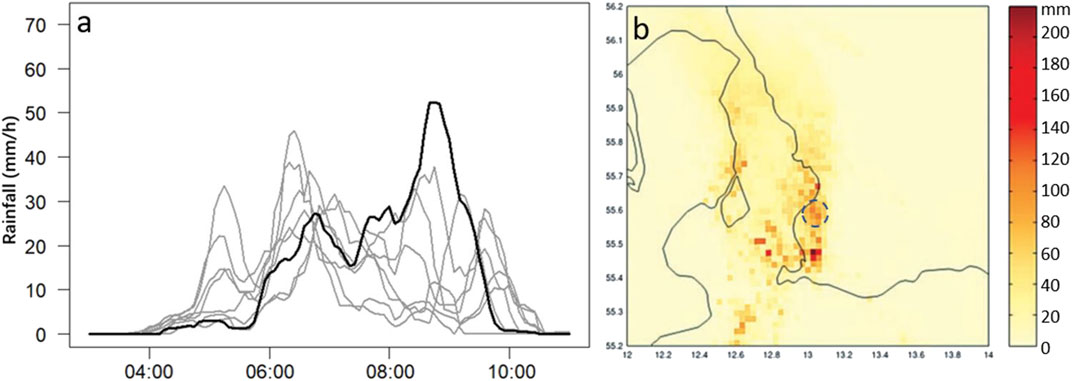
FIGURE 1. Rainfall observed in Malmö at eight permanent observation stations during the extreme event in 2014 (A). The station with the highest peak (Augustenborg) is highlighted to visualise the temporal dynamics. Accumulated rainfall between 04:00 and 10:00 CET on 2014-08-31 as observed by the SMHI weather radar (B) (from Hernebring et al., 2015). The dashed circle shows the location of Malmö.

Local Precipitation Observations

Rainfall data for the period of 1998–2018 were collected from SMHI, seven stations with 15 min rainfall (Table 1; Figure 2C). Precipitation measurements at SMHI stations are conducted by GEONOR automatic precipitation gauges with wind shield. The resolution of the precipitation intensity given by this instrument is 0.1 mm/h and the average relative error of intensity measured by this gauge has been estimated to within ± 2.5% (Vuerich et al., 2009). Following guidelines of the SMHI data distribution center, initial quality control was performed in order to treat erroneous negative precipitation amounts, obviously arisen from the electronic characteristics of the device, were set to missing records (e.g., Jeong et al., 2011).

TABLE 1

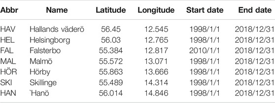
TABLE 1. Rainfall observation stations.

FIGURE 2

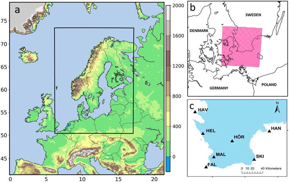
FIGURE 2. The HCLIM12 (outer rectangle) and HCLIM3 (inner rectangle) model domains (A), location of the study region and domain of extracted HCLIM data (in red) (B) and observational stations used in this study (C).

Regional Climate Model Simulations

The small-scale hydrological hazards analyzed in this study are driven by local, short duration and extreme rainfall features. As convection is the key process behind these rainfall extremes, the explicit simulation of convection, and thus the use of convection-permitting regional climate models (CPRCMs), is needed to appropriately reproduce the observed extreme rainfall statistics.

Very recently CPRCM simulations at 3 km have been performed for northern Europe (Figure 2A; Lind et al., 2020). These simulations were performed with the HARMONIE-Climate regional climate modeling system using the version termed cycle38 (HCLIM38), which is described in detail in Belušić et al. (2020). Here we summarize the main characteristics of the simulations. HCLIM38 is based on the HIRLAM-ALADIN numerical weather prediction (NWP) modeling system (Bengtsson et al., 2017; Termonia et al., 2018), with modifications to better suit climate simulations. The hydrostatic and non-hydrostatic dynamical cores, with semi-implicit, semi-Lagrangian discretization and bi-spectral characterization of most prognostic variables are common to the NWP system (Termonia et al., 2018), as are the majority of atmospheric physics options (Seity et al., 2011; Bengtsson et al., 2017; Termonia et al., 2018). The major climate-specific modifications are related to soil and surface physics, focusing on more realistic processes with longer time memory (Belušić et al., 2020).

The HCLIM38 model system provides flexibility as it contains a suite of different model configurations, each adapted for different horizontal grid resolutions. In this study, two configurations are applied; 1) HCLIM38-AROME which is designed for convection-permitting scales (< 4 km) and is used with non-hydrostatic dynamics (Seity et al., 2011; Bengtsson et al., 2017; Termonia et al., 2018); 2) HCLIM38-ALADIN which is the limited-area version of the global model ARPEGE used with hydrostatic dynamics, parameterized deep and shallow convection and is the default option for grid spacings ≳ 10 km (Termonia et al., 2018). For convenience, from now on the shorter HCLIM3 and HCLIM12 acronyms will be used for HCLIM38-AROME and HCLIM38-ALADIN, respectively.

HCLIM12 has been run over a domain covering a large part of Europe and eastern North Atlantic (Figure 2A) on a grid with horizontal resolution of 12 km, 65 levels in the vertical and a time step of 300 s. The lateral boundary data were taken from the global ERA-Interim reanalysis (Dee et al., 2011) on a grid with approximately 80 km resolution in the horizontal, available every 6 h. An atmospheric reanalysis is a three-dimensional gridded dataset obtained by assimilating observational data in a numerical weather prediction model. Reanalyses are considered as the most realistic depictions of the true state of the atmosphere at each given moment that are available on a three-dimensional grid. They provide information on the large-scale environment outside of the regional model domain that constrains the model behavior at the lateral boundaries. The higher resolution simulation was performed using HCLIM3 on a 3-km grid with 65 vertical levels and a time step of 75 s. HCLIM12 provided the lateral boundary data that was used by HCLIM3 every 3 h. The continuous model simulations cover the years 1997–2018, treating the first year as spin-up not used for model evaluation.

From the HCLIM simulations we have extracted the variable total precipitation, i.e., the sum of all precipitation types generated in the HCLIM models, within the domain shown in Figure 2B (the domain differs slightly between HCLIM3 and HCLIM12, due to the different spatial resolutions, but this difference has no impact on the results obtained). The extracted domain thus covers southernmost Sweden and the eastern part of the Danish island Zealand, with 19 × 19 grid boxes for HCLIM12 and 73 × 73 grid boxes for HCLIM3. The HCLIM12 data is available every full hour whereas HCLIM3 has a finer temporal resolution, 15 min. We assume that the sub-domain is sufficiently far away from the HCLIM boundaries to avoid negative effects. If boundary effects extend some six times the grid spacing of the lateral boundary forcing data (Matte et al., 2017), the affected distance becomes 480 km from the HCLIM12 domain and 72 km from the HCLIM3 domain. The distances from the sub-domain (Figure 2B) to the HCLIM boundaries are far longer. For comparison with station observations, time series from the grid cells covering each of the stations (Figure 2C) were extracted from the HCLIM simulations.

Methods

To cover the different purposes of the study, three types of evaluations are performed: intensity-based, time-based and event-based. This “evaluation package” combines metrics commonly used in RCM evaluation with methods and aspects that we believe reflect users’ perceptions of rainfall and particularly short-duration extremes. We will from now on use the term “rainfall” even if some of the annual analyses below includes winter periods with potential snowfall, and thus strictly speaking we are analyzing “precipitation”. However, as the main focus is on summer short-duration extremes, which are associated with liquid precipitation, we use “rainfall”.

Intensity-Based Metrics

The intensity-based metrics are selected to show the ability of HCLIM3 and HCLIM12 to reproduce observed rainfall in three different respects: i) the general rainfall regime, ii) high rainfall intensities, and iii) extreme rainfall intensities. The general rainfall regime is assessed by considering three metrics, the first being average monthly rainfall ${\overline{R}}_{tot}$ (mm/month):

${\overline{\mathrm{R}}}_{\mathrm{tot}}\left(\mathrm{m}\right)=\frac{{\displaystyle {\sum }_{\mathrm{y}=1}^{\mathrm{Y}}{\mathrm{R}}_{\mathrm{tot}}\left(\mathrm{y},\mathrm{m}\right)}}{\mathrm{Y}}(1)$

where m denotes month, y year (Y is the total number of years of data) and R_tot(y,m) the monthly total (i.e., accumulated) rainfall. The second metric is the average monthly wet fraction ${\overline{F}}_{wet}$(%):

${\overline{\mathrm{F}}}_{\text{wet}}\left(\text{m}\right)=100\left(\frac{{\displaystyle {\sum }_{\mathrm{y}=1}^{\mathrm{Y}}\frac{{\mathrm{T}}_{\mathrm{wet}}\left(\mathrm{y},\mathrm{m}\right)}{{\mathrm{T}}_{\mathrm{tot}}\left(\mathrm{y},\mathrm{m}\right)}}}{\mathrm{Y}}\right)(2)$

where T_tot(y,m) denotes the total number of hours and T_wet(y,m) the number of “wet hours”, with a wet hour being defined as an hour with a rainfall intensity > 0.1 mm/h. ${\overline{F}}_{wet}$ thus represents the fraction of all hours in a given month that it typically rains. Finally, we calculate the average monthly wet intensity ${\overline{I}}_{wet}$ (mm/h):

${\overline{\mathrm{I}}}_{\text{wet}}\left(\text{m}\right)=\frac{{\displaystyle {\sum }_{\text{y}=1}^{\text{Y}}\frac{{\text{R}}_{\text{wet}}\left(\text{y},\text{m}\right)}{{\text{T}}_{\text{wet}}\left(\text{y},\text{m}\right)}}}{\text{Y}}(3)$

where R_wet(y,m) denotes the accumulated rainfall from the T_wet(y,m) hours, i.e., the hours defined as wet. The variable ${\overline{I}}_{wet}$ thus represents the typical rainfall intensity in a given month.

High rainfall intensities are represented by high percentiles of the frequency distribution of wet hourly rainfall intensities, i.e., the values used to calculate R_wet. Here we use the 75th, 90th, and 95th percentiles, denoted $I_{wet}^{75}\left(m\right)$, $I_{wet}^{90}\left(m\right)$, and $I_{wet}^{95}\left(m\right)$, respectively (unit: mm/h). Effectively, the percentiles are calculated by pooling all wet hourly intensities from a given month (e.g., all values in June, from all years available), sorting them and identifying the values exceeded by 25% (this value becomes $I_{wet}^{75}$), 10% ($I_{wet}^{90}$) and 5% ($I_{wet}^{95}$) of all intensities.

In the results below, we average the monthly metrics (${\overline{R}}_{tot}, {\overline{F}}_{wet}, {\overline{I}}_{wet}$) over both the entire year (January–Decemeber) and over the summer season (June–August). To describe the difference between the observed time series and the time series simulated by HCLIM3 and HCLIM12 for a certain metric M, we calculate the relative bias (%) of the simulations:

$\mathrm{Bias}= \frac{{\text{M}}_{\text{sim}}-{\text{M}}_{\text{obs}}}{{\text{M}}_{\text{obs}}}\times 100(4)$

where M can be for example the average ${\overline{R}}_{tot}$ in summer.

To assess the ability of HCLIM3 and HCLIM12 to represent extreme rainfall intensities, we examine the reproduction of average annual maximum intensities. These maximum values are calculated for different durations, which in this context means time windows. A moving time window is moved (one time step at the time) over each time series, the rainfall within the time window is accumulated and divided by the length of the time window to convert it to intensity (mm/h). The maximum intensity $I_{max}^d\left(y\right)$ for each year y and duration d is identified, and finally the average value ${\overline{I}}_{max}^d$ is calculated:

${\overline{\mathrm{I}}}_{\text{max}}^{\text{\hspace{0.17em}d}}=\frac{{\displaystyle {\sum }_{\text{y}=1}^{\text{Y}}{\text{I}}_{\text{max}}^{\text{d}}\left(\text{y}\right)}}{\text{Y}}(5)$

In this study, we analyze the durations 15 min, 30 min, 45 min, 1 h, 2 h, 3 h, 6 h, 12 h, and 24 h (for HCLIM12 only 1–24 h as sub-hourly values are not available). This is a standard procedure in the construction of Intensity-Duration-Frequency (IDF) curves widely used in engineering design (e.g., Olsson et al., 2019). In IDF analysis, an extreme value distribution is generally fitted to the annual maxima to estimate values associated with different return periods (i.e., frequency of occurrence). Here we omit this step and as we focus on the annual average value the results reflect the IDF statistics associated with a 1-year return period; in the results we simplify and call the resulting curves Intensity-Duration curves.

Time-Based Metrics (JJA)

Harmonic Analysis (for Diurnal Cycle)

A realistic simulation of the diurnal cycle of rainfall is one of the key aspects of an accurate climate model with regard to the physical processes, especially convection in the summer season (e.g., Jeong et al., 2011). The diurnal variation of rainfall is generally characterized by the daily cycles described by the average rainfall amount ${\overline{R}}_{tot}\left(h\right)$ (mm) and frequency of occurrence ${\overline{F}}_{wet}\left(h\right)$ (%) for each hour h of the day (1 ≤ h ≤ 24). ${\overline{R}}_{tot}\left(h\right)$ and ${\overline{F}}_{wet}\left(h\right)$ are calculated equivalently to Eqs 1, 2, but for each hour of the day instead of for each month of the year. To enable comparisons between the different stations, ${\overline{R}}_{tot}\left(h\right)$ and ${\overline{F}}_{wet}\left(h\right)$ were normalized into ${\overline{R}}_{tot}^{nor}\left(h\right)$ and ${\overline{F}}_{wet}^{nor}\left(h\right)$ by division with the corresponding 24-h average values (Yin et al., 2009).

In this study, the diurnal cycle during the summer (June–August) was analyzed using a harmonic analysis. The most important characteristics of the diurnal cycles are i) the peak timing PT and ii) the amplitude AM, where PT defines the hour with maximum rainfall amount or frequency and AM quantifies the range of variation over the day. To determine PT and AM, smoothed cycles of ${\overline{R}}_{tot}^{nor}\left(h\right)$ and ${\overline{F}}_{wet}^{nor}\left(h\right)$ at each station were calculated by using the harmonic analysis technique. A modeled diurnal variation can be represented by the summation of sinusoidal harmonics as (Yin et al., 2009; Jeong et al., 2011):

$\overline{\mathrm{R}}\_\text{har}\left(\text{h}\right)=\overline{\overline{\mathrm{R}}}+{\displaystyle \sum }_{\text{k}}{\text{C}}_{\text{k}}\cos \left(\frac{2\mathrm{\pi }\text{kh}}{24}-{\mathrm{\theta }}_{\text{k}}\right)+\text{residual}(6)$

$\overline{\mathrm{F}}\_\text{har}\left(\text{h}\right)=\overline{\overline{\mathrm{F}}}+{\displaystyle \sum }_{\text{k}}{\text{C}}_{\text{k}}\cos \left(\frac{2\mathrm{\pi }\text{kh}}{24}-{\mathrm{\theta }}_{\text{k}}\right)+\text{residual}(7)$

where $\overline{\overline{R}}$ and $\overline{\overline{F}}$ are the 24-h means of ${\overline{R}}_{tot}^{nor}\left(h\right)$ and ${\overline{F}}_{wet}^{nor}\left(h\right)$. The variable k is the harmonic number, with k = 1 representing a harmonic with a 24-h period, k = 2 a 12-h period, etc. Variables C_k and θ_k are the amplitude and the phase, respectively, of a given kth harmonic. In this study, the summation of the first (k = 1) and second part (k = 2) of the harmonics was used to define the smoothed diurnal cycle, which is common practice (e.g., Jeong et al., 2011). The amplitude of this smoothed diurnal cycle was determined as half of the difference between the maximum and minimum value within the 24-h cycle, and the peak timing was determined as the time when the maximum value occurs. More details of the mathematical representations can be found in Yin et al. (2009), Jeong et al. (2011).

To clarify the output from the harmonic analysis of the diurnal cycle, Figure 3 shows an example from the results, for rainfall occurrence at station HEL. In this case, the fitted final harmonics (solid lines) well represent the hour-by-hour empirical values (dotted lines), with an average explained variance of 0.70. Over all time series (observations, HCLIM3, HCLIM12) and harmonic variables (PT, AM), the explained variance ranges between 0.43 and 0.78 which agrees with previous work (Jeong et al., 2011).

FIGURE 3

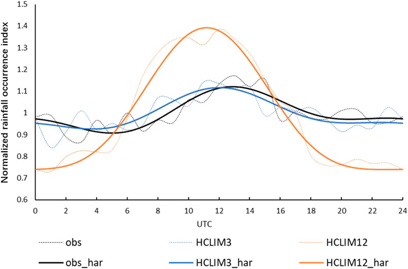
FIGURE 3. Example of empirical cycle (dotted lines) and smoothed cycle by harmonic analysis (solid lines) for rainfall occurrence in station HEL.

Intra-Seasonal Distribution of Annual Maxima

Malmö is located on a flat coastal area where the occurrence of short-duration rainfall extremes is associated with thermal and circulation conditions that favor the formation of rainfall, especially convection. During the summer convection may be enhanced by sea breeze, otherwise, the passage of mesoscale meteorological events is the main responsible for heavy rainfall. Therefore, the monthly occurrence of the rainfall extremes, i.e., in which months they occur, is an important characteristic for evaluating climate model performance. In this study, the percentage of extremes occurring in each summer month (June–August) was calculated and analyzed.

Annual maxima for different durations d (1, 2, 3, 6, 12, and 24 h) were identified in the above Intensity-Duration analysis (Intensity-Based Metrics) and here we analyze the calendar month m in which these maxima occurred, $m_{max}^d\left(y\right)$. For each month, the occurrences of annual maxima in all years were summed according to:

${\text{O}}_{\text{max}}^{\text{d}}\left(\text{m}\right)=\{\begin{array}{ll}0\hfill & {\text{m}}_{\text{max}}^{\text{d}}\left(\text{y}\right)\ne \text{m}\hfill \\ 1\hfill & {\text{m}}_{\text{max}}^{\text{d}}\left(\text{y}\right)=\text{m}\hfill \end{array}(8)$

after which the percentage of annual maxima in each month were calculated as:

${\text{Perc}}_{\text{max}}^{\text{d}}\left(\text{m}\right)=\frac{{\text{O}}_{\text{max}}^{\text{d}}\left(\text{m}\right)}{\text{Y}}\times 100(9)$

Reproduction of Historical Events

All users and practitioners dealing with weather in some form are familiar with specific historical and “(in-)famous” events, remembered mainly because of their consequences, e.g., heavy rain flooding basements, strong winds felling trees or long dry periods causing drought. Generally, the meteorological conditions behind these events are extreme or at least very unusual. For users, historical events are very important as “prototypes” as a means to analyze and understand the vulnerability of their city or forest or water source to weather hazards. Concerning “weather models”, whether for short- or long-term forecasting or for climate projections, a natural and understandable question from a user is “can this model simulate an event such as the one we experienced X years ago?”. If the answer is “yes”, this will increase the user’s confidence in the model, and vice versa. The prospect of event-based evaluation of long-term simulations has been previously explored (e.g., Berthou et al., 2020) but the approach is complex with several pitfalls. In this paper we try to describe, illustrate and discuss this complexity by using the Malmö event (Study Area and Data) as a case study.

In our case, as the HCLIM models are continuously forced with a meteorological reanalysis that is based on observations, for a non-expert it is reasonable to assume that the model output should fairly well agree with observations also within the domain, on any given time and place. In reality however, the forcing is given only at the lateral boundaries. Within these boundaries the RCM can develop its own atmospheric state and phenomena. This RCM state could considerably differ from the reanalysis in the interior of the domain but still agree with the boundary forcing. This is, generally speaking, not a drawback but an added value of the higher resolution in the RCM which allows for a more detailed representation of atmospheric systems and underlying surface.

The level of agreement one can expect highly depends on both the variable considered and on the scale of the atmospheric systems involved. In terms of rainfall, when it is generated by large-scale weather systems, such as warm fronts, some agreement can be expected at a certain time and place, or at least in its vicinity. This is because these large-scale systems are present in the coarser reanalysis and are therefore manifested in the domain boundaries as incoming weather systems. The RCM domain is usually too small to develop a completely independent state at these scales. However, when rainfall is generated by small-scale systems, such as local thunderstorms, the agreement with observations is not expected. This is because these systems are not present in the reanalysis and hence are not represented at the model boundaries, and the RCM can generate them itself anywhere inside the domain when favourable conditions exist. Therefore, instead of expecting that a specific historical heavy rainfall event should be reproduced at exactly the same place and time as in reality, it is more appropriate to desire that given the correct large-scale information, the model correctly reproduces the ensemble of different rainfall events over a certain region and over a longer time period (e.g., a few decades), i.e., that the model correctly reproduces the distributions of intensity, duration and diurnal cycle of rainfall events.

Thus, the possibility to find a specific historical rainfall event in the HCLIM simulations is totally dependent upon the scale of the atmospheric processes involved in the generation of the event. In our case, the Malmö event includes a combination of processes at different scales, with small-scale convective cells embedded in a large-scale frontal system (Study Area and Data). As the event has a large-scale component, it is à priori reasonable to assume that the models will generate some rainfall in the region, around the same time as it was observed. However, as the high intensities were generated by convection there is no reason to expect any high-intensity rainfall particularly in Malmö or its vicinity.

We thus cannot expect the HCLIM models to fully reproduce the Malmö event at the right time and place, but can we expect them to generate a Malmö event at some other time and place during the 20-year simulation period? Generally, an arbitrary 20-year period cannot be expected to contain events with a longer return period than 20 years, i.e., events larger than the one which occurs on average once every 20 years. In a given 20-year simulation, the maximum event will most probably have a return period which is either longer or shorter than 20 years, because of natural variability. Then, what is the estimated return period of the Malmö event? This estimation is very difficult for different reasons. First of all it depends on how the event is defined, in terms of duration and spatial extension. A given rainfall event will have different return periods for different combinations of duration and area. Secondly, the amount of high-resolution observations available in the region is limited, and therefore there is huge uncertainty in observation-based estimates of intensities associated with long return periods. Considering the Malmö event, available estimates indicate a return period of up to several hundred years for the “worst” duration (∼6 h), but with a confidence interval having a lower limit of around 40 years (Olsson et al., 2017a). This is an estimation for a given location; for a region like the domain used in the simulations here (Figure 2B) it becomes different. The return period for a specific event occurring anywhere within the domain will be shorter but how much shorter is highly uncertain. In summary, we cannot expect the Malmö event to be reproduced in a given 20-year simulation. If the event anyway happens to be reproduced in a certain simulation, this cannot be considered as “right” or “wrong” but the only relevant conclusion is that the model is able to simulate this type of event.

Below we investigate i) the rainfall generated by the HCLIM3 and HCLIM12 models on the day of the Malmö event (2014-08-31) and ii) whether rainfall events of the same magnitude as the Malmö event are present anywhere in the HCLIM3 and HCLIM12 simulations. As the duration of the Malmö event was 6 h and the maximum observed accumulated rainfall 122 mm (Study Area and Data), we use these numbers to define the event. Similar to the analysis of annual maxima (Intensity-Based Metrics), we use a moving 6-h time window to identify accumulations larger than 122 mm in all grid cells within the model domain for the entire simulation period.

Results and Discussion

Intensity-Based Metrics

Table 2 gives an overview of the rainfall climate in Scania, as described by the intensity-based metrics (Intensity-Based Metrics) during the period 1998–2018. Both annually and in summer, total rainfall ${\overline{R}}_{tot}$ is highest in central Scania (station HÖR) and along the northern west coast (HAV, HEL), whereas the lowest values are found in the south-west (FAL) and in the east (HAN, SKI). The variation of the wet fraction ${\overline{F}}_{wet}$ overall follows the same pattern as ${\overline{R}}_{tot}$. The average wet intensity ${\overline{I}}_{wet}$ is somewhat higher along the west coast than on the east coast and the pattern is most clear in summer. Also the high percentiles $I_{wet}^{75}$, $I_{wet}^{90}$, and $I_{wet}^{95}$ generally have larger values in the west than in the east. For the highest percentiles (90, 95) the differences are small, but the values in the east coast (SKI, HAN) are generally lower than the rest. Overall, the rainfall is thus slightly more frequent with slightly higher intensity in the “north-west-central” part of Scania (HAV, HEL, MAL, HÖR).

TABLE 2

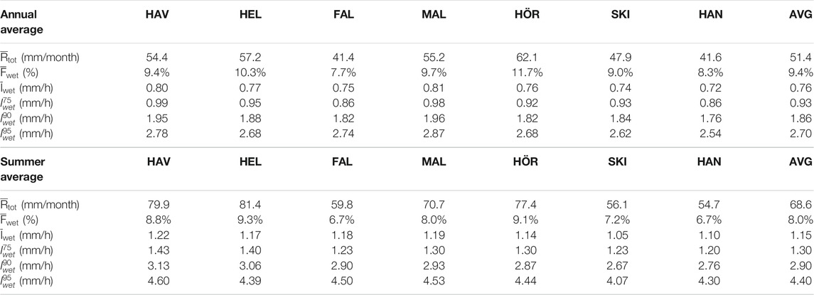
TABLE 2. Annual and summer (June–August) averages of the intensity-based metrics for observed rainfall in each station and on average over all stations (AVG). Table 1 shows the periods of averaging.

Figure 4 shows the bias of ${\overline{R}}_{tot}$, ${\overline{F}}_{wet}$, and ${\overline{I}}_{wet}$ in HCLIM3 and HCLIM12. If first looking at ${\overline{R}}_{tot}$ (Figure 4A) and the annual values, HCLIM12 shows a consistent overestimation by 27% on average, ranging from 40% in the north-western part of the domain (HAV) to 15% in the south-east (SKI). In HCLIM3, the bias is greatly reduced to 2% on average with small differences between the stations. We note that gauge undercatch, i.e., the fact that precipitation (especially in the form of snow) may not enter the gauge because of winds around the gauge, can have some impact on the annual analysis. However, the impact is likely small and we neglect it here (see further Discussion). For summer, the bias pattern in HCLIM12 is similar to the annual pattern but the values are lower, being on average 14%. In HCLIM3, some underestimation is apparent especially in the west (HAV, HEL, MAL, FAL) and the average bias over all stations is −11%.

FIGURE 4

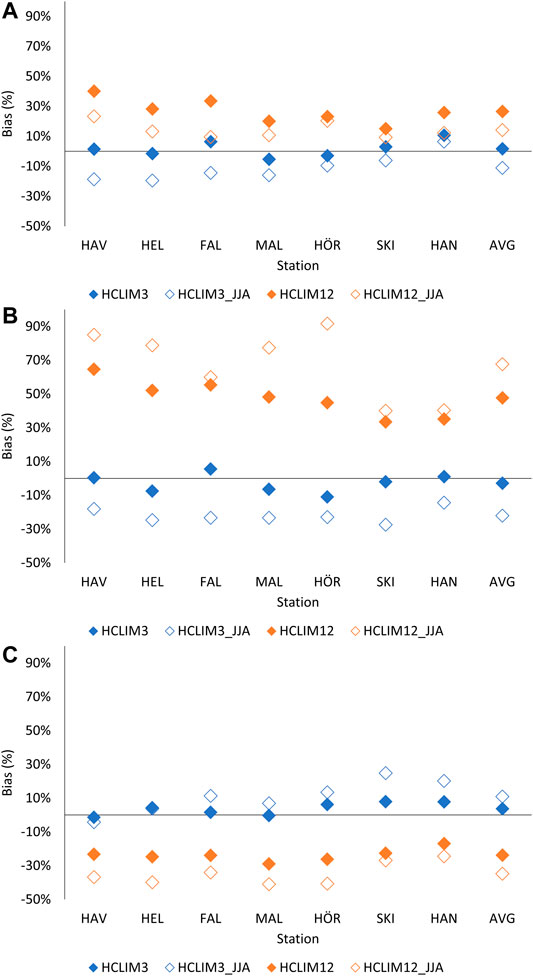
FIGURE 4. Bias of 1-h rainfall of HCLIM3 and HCLIM12 in each station: total monthly precipitation ${\overline{\mathrm{R}}}_{\mathrm{tot}}$(A), wet fraction ${\overline{\mathrm{F}}}_{\mathrm{wet}}$(B) and wet intensity ${\overline{\mathrm{I}}}_{\mathrm{wet}}$(C). Diamonds with filled color denote annual averages, diamonds without fill denote summer (June–August) averages.

The annual wet fraction ${\overline{F}}_{wet}$ (Figure 4B) is substantially overestimated in HCLIM12, by up to 65% at HAV and by 48% on average. In summer, the overestimation is even more pronounced, up to 92% at HÖR. On the annual scale, HCLIM3 has only a small negative bias on average (−3%) with small differences between the stations. In summer, a consistent negative bias between −14 and −27% is found in HCLIM3.

From the results in Figures 4A,B it is apparent that HCLIM12 generally underestimates the intensity of wet hours, which is confirmed in Figure 4C. HCLIM3, on the other hand, overall well matches the observations in this respect, although with some overestimation in the east (HAN, SKI).

To assess the performance for intense rainfall, we investigate the high percentiles of non-zero values; $I_{wet}^{75}$, $I_{wet}^{90}$, $I_{wet}^{95}$ (Figure 5). On the annual scale, HCLIM12 substantially underestimates the high percentiles, to an increasing degree with increasing percentile, up to −35% on average for $I_{wet}^{95}$ (Figure 5A). HCLIM3 shows only a limited bias, between −7 and 8% over all stations and percentiles, and on average HCLIM3 is virtually unbiased. In summer (Figure 5B), the underestimation by HCLIM12 becomes further pronounced with biases reaching −52% (HÖR) for $I_{wet}^{95}$ although lower in the east (HAN, SKI). Concerning HCLIM3, on average some overestimation is found for the high percentiles in summer, by 7% on average, reaching up to 30% for $I_{wet}^{95}$ at SKI. There is a geographical pattern with distinct overestimations in the east (HAN, SKI) and even a slight underestimation in the north-west (HAV, HEL).

FIGURE 5

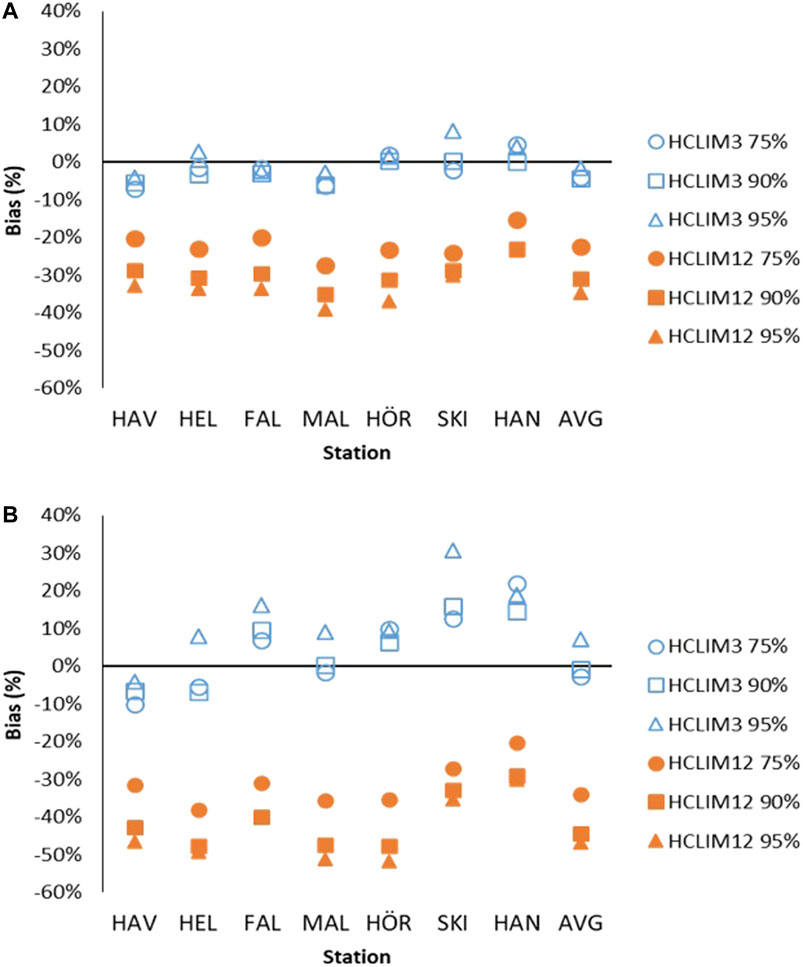
FIGURE 5. Bias of 1-h rainfall percentiles ${\mathrm{I}}_{\mathrm{wet}}^{75}$, ${\mathrm{I}}_{\mathrm{wet}}^{90}$ and ${\mathrm{I}}_{\mathrm{wet}}^{95}$ in HCLIM3 and HCLIM12 for annual averages (A) and summer (Jun-Aug) averages (B). Circle, square and triangle represent percentile 70, 90, and 95, respectively.

Figure 6 shows the observed and simulated Intensity-Duration (ID) curves. Looking first at HCLIM12, generally the simulated intensities match the observed ones for the longer durations 6–24 h, as evident from the average curve (Figure 6H). For shorter durations, in general HCLIM12 gradually deviates from the observed ID curves, and at duration 1 h the HCLIM12 intensity is approximately half of the observed one. Overall, HCLIM3 well matches the observed ID curves (Figures 6A–D). Some overestimation is however apparent for durations around 1 h in the eastern stations (Figures 6E–G), in line with the overestimated $I_{wet}^{95}$ at these stations (Figure 5B). Furthermore, at duration 15 min the observed intensities are nearly always underestimated by HCLIM3, the exception being at SKI (Figure 6F). The underestimation is up to −27% at MAL (Figure 6D) with an average value of −13% (Figure 6H).

FIGURE 6

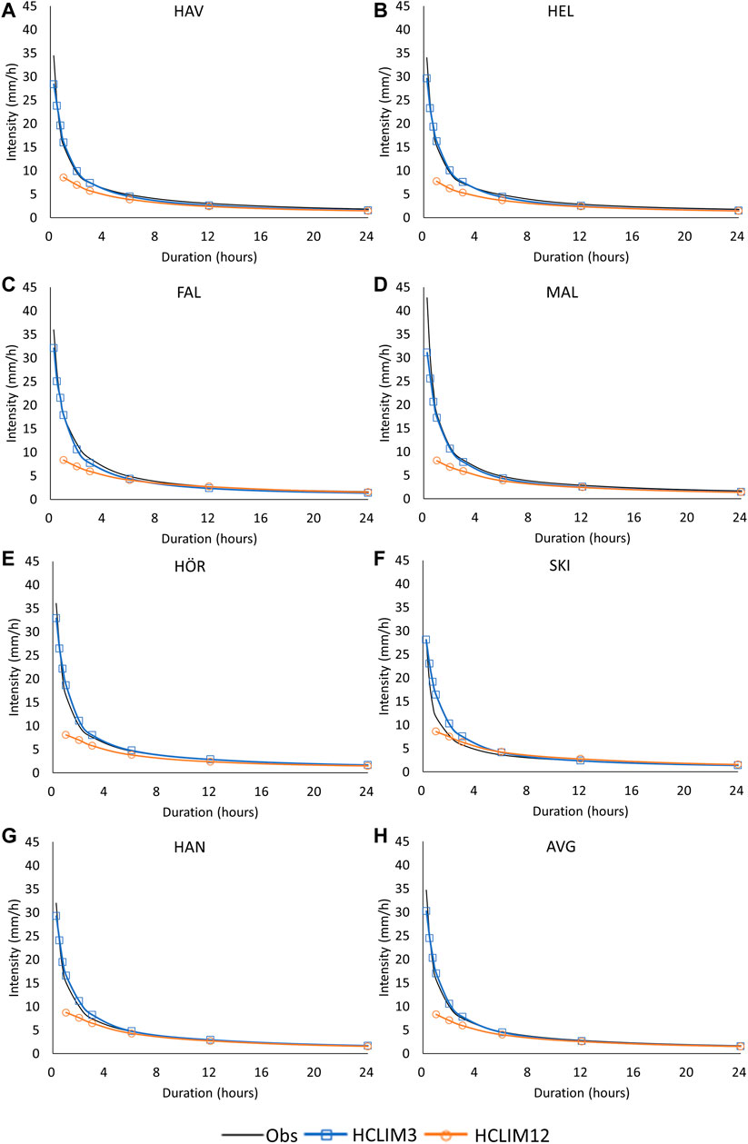
FIGURE 6. Intensity-Duration curves of observed and simulated average annual maxima in stations HAV (A), HEL (B), FAL (C), MAL (D), HÖR (E), SKI (F) and HAN (G) as well as on average over all stations (H).

An important aspect when comparing extreme rainfall intensities from different sources is any difference in spatial resolution. Statistical extremes from a point source, e.g., a gauge, will be higher than extremes from a “spatial source”, e.g., a weather radar or a climate model, because of spatial averaging in the latter. This means that we expect the extremes from HCLIM3 and HCLIM12 to be lower than the station-based extremes, but the difference is small and/or uncertain and we neglect it here (see further Discussion).

Time-Based Metrics (JJA)

Figure 3 shows an example of the diurnal cycle, estimated for rainfall occurrence at HEL. The diurnal cycle derived by the first and second harmonics well represents the estimated amplitude and peak phase in the observations. In the case of HEL, the HCLIM3 cycle is substantially closer to the observed cycle than the HCLIM12 cycle in terms of amplitude, whereas the peak timing is similar (Figure 3).

Table 3 shows the characteristics of the smoothed diurnal cycle at all seven stations. Looking first at rainfall amount, the amplitude in the observations ranges between 0.06 (MAL) and 0.25 (HÖR). This indicates that high rainfall intensities at HÖR are more concentrated to a certain part of the day, giving a distinct daily cycle, whereas at MAL they happen at different times and the cycle becomes flatter and less distinct. In general, the amplitude is somewhat lower at the western stations (HAL, HEL, FAL, MAL). The average amplitude in the observations is 0.17 and this value is well reproduced by HCLIM3 (0.15), although the observed spatial pattern is not clear in HCLIM3. HCLIM12 well describes the amplitude at the eastern stations (SKI, HAN) but generally overestimates it at the rest of the stations, and the average value is 0.25. The mean absolute error (MAE) in HCLIM3 (0.06) is half of that in HCLIM12 (0.12).

TABLE 3

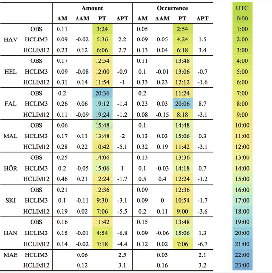
TABLE 3. Amplitude (AM) and peak timing (PT) of rainfall amount and occurrence in each station in the observed (OBS) and simulated (HCLIM3, HCLIM12) smoothed diurnal cycles. ΔAM and ΔPT represent the difference between observed and simulated values and their Mean Absolute Error (MAE) is given in the bottom. The color bar on the right denotes the time of day (UTC).

In terms of peak timing of the rainfall amounts, this varies gradually and rather widely in the western part of Scania, from 03:24 at the northern station (HAV), through 12:54 and 15:48 at the central stations (HEL, MAL), to 20:36 at the southern station (FAL). At the other station, the peak is around noon or early afternoon. HCLIM3 manages to well reproduce the distinct pattern in the western part, with an average difference of only 0.5 h. At the eastern stations (SKI, HAN), however, the peak occurs 3–7 h earlier in HCLIM3. The results for HCLIM12 are qualitatively similar to the ones for HCLIM3, but the MAE (3.1 h) is slightly higher than the one for HCLIM3 (2.5 h).

Turning to rainfall occurrence, the observed amplitudes are generally smaller than for rainfall amount, i.e., the cycles are smoother. The average amplitude is 0.12 and with some exceptions the differences between stations reflects the differences found for rainfall amount. HCLIM3 reproduces the observed amplitudes very well, the average value is identical (0.12) and the MAE = 0.03. Similarly to rainfall amounts, HCLIM12 overestimates the amplitude for the west-central stations, and the average value is 0.24 (MAE = 0.16). The observed peak timing for rainfall occurrence is generally similar to the one for amount, the exception being station FAL where occurrence peaks at around noon in contrast to the evening peak of the amount. Overall, HCLIM3 reproduces the occurrence peak times slightly better than the amount peak times, with MAE = 2.1 h, although it fails to capture the difference at station FAL. HCLIM12 better manages to capture this difference, but overall the performance is worse than for HCLIM3, evidenced by a MAE of 3.2 h.

Figure 7 shows the intra-seasonal occurrence of sub-daily extremes, as expressed by the percentage of annual maxima $Per{c}_{max}^d$ in each summer month (June–August). Looking first at HAV (Figure 7A), in the north-west, we see first of all that all extremes happen in summer as all bars add up to 100%. At duration 1 h, most of the annual maxima (57%) happen in August, followed by July (29%) and June (14%). As duration increases, the fraction of maxima in August gradually decreases to 24% at duration 24 h, whereas the fraction in July increases substantially, to 52%, and the fraction in June increases somewhat less, to 24%. Concerning HCLIM3, the fraction of maxima in June is overestimated, by 19% percentage points, whereas the fractions in July and August are underestimated. The overestimation in Jun is consistent over all durations but the observed changes in July and August at longer durations is overall qualitatively reproduced by HCLIM3, although not as clearly. HCLIM12 somewhat better captures the observed pattern at durations 1–6 h, but at the longer durations the fraction in August is overestimated and the fraction in Jun underestimated. In total, HCLIM12 performs slightly better with MAE = 6% for the monthly fractions, compared with 9% for HCLIM3.

FIGURE 7

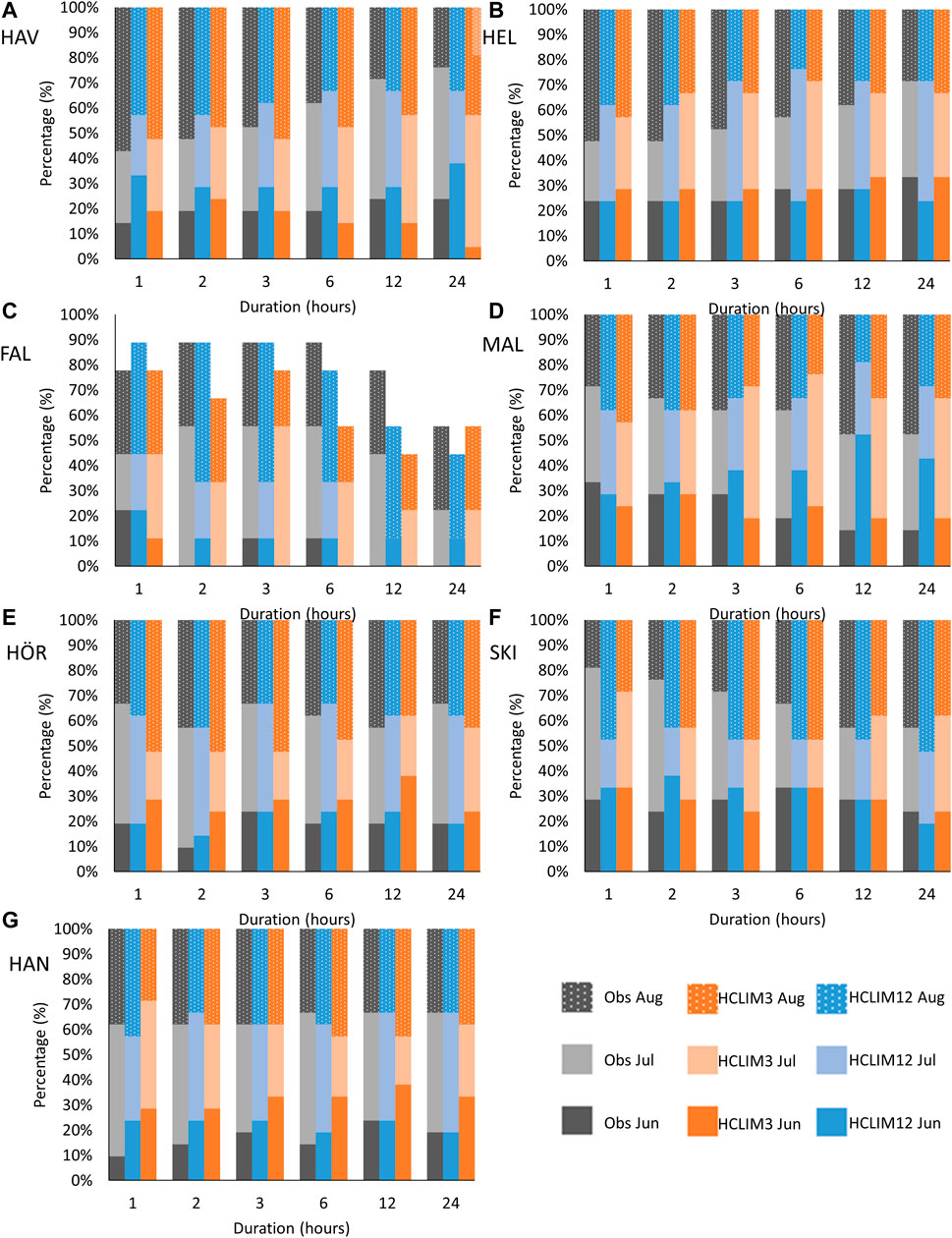
FIGURE 7. Percentage of annual extremes $\mathrm{Per}{\mathrm{c}}_{\max }^{\mathrm{d}}$ in Jun, Jul and Aug for durations 1, 2, 3, 6, 12, and 24 h in stations HAV (A), HEL (B), FAL (C), MAL (D), HÖR (E), SKI (F) and HAN (G).

At station HEL (Figure 7B), the observed pattern is overall similar, with the fraction of maxima in August decreasing with increasing duration, and the fractions in June and July increasing. The average fraction in June is well captured in HCLIM3, whereas the fraction in July is overestimated and in August underestimated, leading to an average MAE of 10%. The behaviour of HCLIM12 is qualitatively similar but with a slightly lower MAE of 7%.

Station FAL (Figure 7C) stands out as the only station where not all maxima occur in summer, but only 80% in average over all durations, which makes these results more uncertain than the results from the other stations. At 24 h duration, just over half of the annual maxima occur in summer. Over all durations, the fraction in August is 33%, the fraction in Jun is small or even zero, and the fraction in Jul varies between 20 and 60%. Both HCLIM3 and HCLIM12 are able to reproduce the fact that not all extremes occur in summer; in HCLIM3 on average 74% occurs in summer and in HCLIM12 63%. Concerning the overall pattern, HCLIM3 generally underestimates the fraction in Jul and overestimates in June and August. Overall HCLIM12 has a somewhat better reproduction of the observed pattern and a lower MAE.

At MAL and SKI (Figures 7D,F), the fraction of maxima in Aug increases with increasing duration, from 20 to 30% at duration 1 h to 40–50% at 24 h. At MAL, the fraction in Jun decreases with duration whereas the fraction in Jul is rather constant; at SKI it is the other way around. Neither HCLIM3 nor HCLIM12 is able to fully describe the patterns and again MAE for HCLIM12 is a few percentage points lower than for HCLIM3.

Finally, at HÖR and HAN (Figures 7E,G) there is no clear dependence on duration, but ∼17% of the maxima occurs in June, ∼46% in July and ∼37% in August. Especially at HÖR, this (absence of) pattern is very well reproduced by HCLIM3 with MAE = 2%, which is a distinct improvement compared with MAE = 14% for HCLIM12. Also at HAN, HCLIM3 (MAE = 5%) clearly outperforms HCLIM12 (MAE = 13%). In total, averaged over all stations MAE for HCLIM12 is a few percentage points lower than for HCLIM3.

Evaluation of the Malmö Event

Looking first at the model results for the same day as the Malmö event, i.e., 2014-08-31 (Figure 1), it is clear that rainfall was indeed generated in the region by both HCLIM3 and HCLIM12 (Figure 8). In HCLIM3, a band with peak accumulations up to 40 mm exists north of Malmö, and also one high-intensity spot happens to be located over Malmö city. In HCLIM12, somewhat lower peak accumulations are found in the north-eastern part of the domain. The differences can be explained by different structures of the storm in the two simulations, even though the large-scale features of the main frontal systems are similar. In HCLIM12, the majority of rainfall occurs along the front in a narrow band. Since the front passes over Malmö around 20 UTC on 30 August and moves eastward, the accumulated rainfall shown for 31 August does not include its effects over Malmö but only further east. On the other hand, in HCLIM3 the majority of rainfall comes from the organised individual convective systems that are trailing the front. These organised systems provide a twofold distinction compared to HCLIM12: they have stronger local rainfall maxima and they appear after the front passage.

FIGURE 8

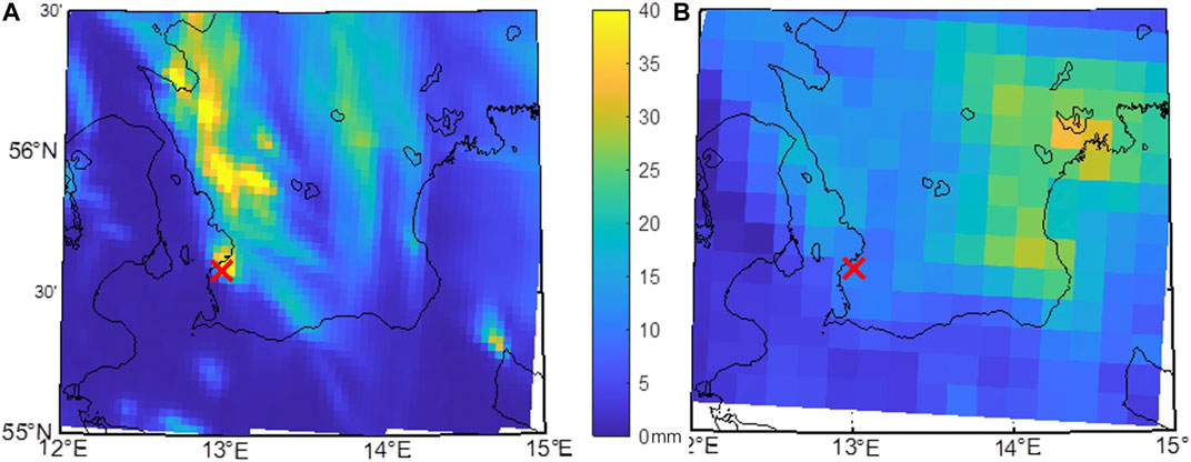
FIGURE 8. Accumulated daily rainfall simulated by HCLIM3 (A) and HCLIM12 (B) on 2014-08-31 (the Malmö event). The red cross shows the location of Malmö.

The search for Malmö events, i.e., more than 122 mm in 6 h, in the entire simulations generated one “hit” in the lower central part of the domain by HCLIM3 (Figure 9A), on 2002-08-03. This event is similar to the actual Malmö event, with a spatial structure suggesting an organized convective system resulting in an extended period with high intensities and multiple peaks. Also the time of day, 4–10 a.m., is virtually identical. An obvious question becomes: what was actually observed on this day? The observations from the station network in Scania confirm that intense rainfall indeed occurred in the period of the simulated event, i.e., 2002-08-03 a.m. (Figure 9B). The accumulated rainfall ranges from 0 (HAN) up to almost 30 mm (SKI). The highest short-duration intensity was actually registered in Malmö (MAL) and the local gauge network in Malmö recorded accumulations up to almost 50 mm. This caused local flooding in the city which is evidenced by 75 flood claims being reported (Sörensen and Mobini, 2017).

FIGURE 9

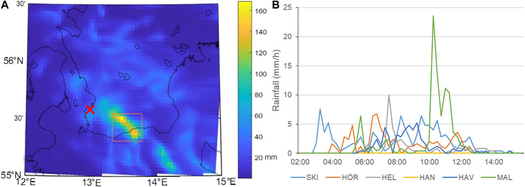
FIGURE 9. Accumulated rainfall between 02:00 and 14:00 UTC on 2002-08-03 as simulated by HCLIM3 (A) and the rainfall observations from the station network in the same period (B). The red cross shows the location of Malmö.

Two more events above the criterion 122 mm in 6 h were found in the HCLIM3 simulation; one highly localized event on 2014-07-07 with 6-h accumulations reaching 200 mm in and one more clustered event on 2002-08-03 with 6-h accumulations reaching just a few mm above 122 mm. Both these events are, however, cut off at the northern boundary of the domain and were thus incompletely represented in this analysis.

In the HCLIM12 simulation no events of the same magnitude as the Malmö event were found. The largest event found however reached above 100 mm in 6 h, which is a very significant rainfall. This is in line with Figure 5, showing that HCLIM12 overall well reproduces 6-h maxima in a statistical sense, whereas the results presented in this section indicate that the largest events are not fully captured.

Discussion

A number of adjustments or corrections are possible when comparing rainfall observations and climate model output, related to different aspects of the data. One aspect is gauge undercatch, i.e., that the wind field around the gauge makes some of the rainfall miss the gauge. In Sweden, the undercatch can be substantial especially in the north during winter, when precipitation falls as snow. For southern Sweden the effect is smaller, especially for high intensities in summer which is the focus in this study (e.g., Olsson et al., 2019). Even if undercatch may have some influence on the annual results related to total precipitation and wet fraction (Figures 4A,B), the adjustment needed is highly uncertain.

Another possible adjustment is for spatial and temporal differences in the data; observations (point values; 15-min), HCLIM3 (9 km²; 15-min) and HCLIM12 (144 km²; 1-h). This area has a known impact on short-duration extreme intensities and in some studies correction factors are applied, e.g., so-called Areal Reduction Factors (ARFs) (e.g., Berg et al., 2019). In this study, the spatial difference is likely to have an impact mainly on the Intensity-Duration curves (Figure 6) and possibly also the high percentiles (Figure 5). However, also in this case the values of the adjustment factors are uncertain and there are different suggestions in the literature (e.g., Pavlovic et al., 2016). Conceivably, the adjustment needed for HCLIM3 is small and may be neglected whereas for HCLIM12 it may be around 10% or more (e.g., Pavlovic et al., 2016). Concerning temporal differences, the time step in the data will have an impact on the maximum values estimated by a moving time window, but based on previous studies the impact of this particular time step difference is small (e.g., Berg et al., 2019).

As none of the above potential adjustments will change any conclusions from the study, and as the adjustments needed are small and/or uncertain, we prefer not to adjust but only comment in text when an adjustment may be relevant. Thus, we assess what comes out of the models directly, which also has the advantage of being transparent and “non-disturbed”.

The results obtained in the intensity-based analyses are overall in line with previous findings and knowledge about rainfall (precipitation) in climate models including HCLIM3. The added value offered by CPRCMs is most clearly seen for wet fraction and annual maxima, but also for seasonal and annual biases which are not always improved by CPRCMs (e.g., Prein et al., 2013). The improved biases are overall consistent with the results in Lind et al. (2020), who evaluated HCLIM3 and HCLIM12 over the HCLIM3 domain using different observational data sets. However, some of our results are region-specific and may look different on the scale of the entire domain. For example, the dry bias of HCLIM3 in summer is mostly confined to the southern parts of the domain including the region analyzed here.

Other results are consistent across the domain e.g., the overestimation of precipitation in HCLIM12, which is caused by the overestimation of weak to moderate precipitation. This “drizzle effect” is manifested in the overestimated wet fraction in HCLIM12 (Figure 4B). Even if the amount of “accumulated drizzle” is relatively small, if uncorrected it will affect subsequent impact modeling, e.g., by a consistently overestimated soil moisture. In practice the drizzle effect is generally reduced by some bias adjustment method prior to subsequent application (e.g., Yang et al., 2010), but this adds uncertainty to the results. Also the substantial underestimation of high percentiles and annual maxima in HCLIM12 agrees with previous studies (e.g., Berg et al., 2019). This underestimation raises concerns about the accuracy in e.g., today’s RCM-based climate factors that are widely used in engineering to take future increase into account.

Also in terms of the diurnal cycle of rainfall amount and occurrence, HCLIM3 showed a notable improvement compared with HCLIM12, especially in terms of the cycles’ amplitude but also the peak timing. Being a key metric in climate model evaluation, the diurnal cycle is sensitive to many interacting physical processes involved in rainfall generation (e.g., Lind et al., 2020). Overall, HCLIM3 did not improve performance with respect to the monthly occurrences of annual maxima in summer (Figure 7), except in the central station HÖR. We encourage more analyses and climate model evaluation focusing on monthly occurrence patterns of rainfall extremes with different duration, as this is another direct reflection of the physical processes.

Concerning the evaluation based on the Malmö event, the results showed first of all that the HCLIM3 and HCLIM12 models did generate rainfall in the region on 2014-08-31, which was expected because of the large-scale component involved in the generation of the event (e.g., Berthou et al., 2020). The daily accumulations in both models were substantially lower than the maximum observed accumulation, but the higher values in HCLIM3 than in HCLIM12 are conceivably related to the explicit description of convection in HCLIM3. As both location and magnitude of the simulated peak accumulations are essentially governed by chaotic processes and we can from this analysis not draw any firm conclusion about one simulation being superior to the other (Reproduction of Historical Events). When analyzing the full simulation periods, at least one Malmö event was found in the HCLIM3 simulation whereas no event was found in the HCLIM12 simulation. Neither from this result we can conclude that HCLIM3 is superior, both because of the impact of random variability and because of uncertainties associated with characterizing the event (Reproduction of Historical Events). What we can conclude, however, is that HCLIM3 is able to simulate events like the one in Malmö 2014 in the same region, whereas we cannot confirm whether this is the case also for HCLIM12.

We close this section with some reflections concerning the general question whether we can expect to find a specific event in simulations, even if the estimated return period of the event is longer than the simulation period. The answer is related to the scale of the event and to which degree the event is associated with or governed by the climate model boundaries (Reproduction of Historical Events). In a general sense, the boundary conditions themselves will have a certain return period, that may make them particularly favourable for generating a certain type of (extreme) event. If there is a strong link between the boundaries and the type of event considered, e.g., large-scale rainfall, there is a high probability of a corresponding event materializing in a given simulation. For convective-type rainfall, the link is much weaker and random variability will have a larger impact. For (extreme) events associated with other hazards, e.g., drought and wildfires following extended warm and dry periods, other types of dependence on boundary conditions will exist, in turn affecting the possibility to reproduce an event in RCM simulation. Further exploration of this prospect may be a way to bring climate model evaluation closer to users.

Summary and Conclusion

We have evaluated historical simulations by two regional climate models–HCLIM3 (3 × 3 km², non-hydrostatic, convection-permitting) and HCLIM12 (12 × 12 km², hydrostatic)–with respect to their reproduction of rainfall in southern Sweden. The main improvements obtained by the HCLIM3 model were the following.

• Intensity-based evaluation: A substantially improved reproduction of both long-term statistics (accumulation, wet fraction) and high or extreme short-duration intensities.

• Time-based evaluation: An improved representation of the daily cycle of rainfall amount and occurrence, especially the amplitude but also the peak time.

Furthermore at least one event of a magnitude similar to the one that occurred in Malmö 2014-08-31 was simulated by HCLIM3 but not by HCLIM12. This can however not be considered an unambiguous improvement because of uncertainties and randomness involved in event-based evaluation. In terms of monthly occurrences of annual maxima, no clear added value was found in the HCLIM3 simulation.

We conclude that overall the convection-permitting HCLIM3 model is able to represent local, and particularly extreme, rainfall with a high accuracy. This will be beneficial in several respects, as compared with today’s RCM simulations and projections. Concerning subsequent impact modeling, even if bias adjustment generally will still be needed it is likely to become less “disturbing” with a smaller additional uncertainty. The greatly improved representation of short-duration extremes opens up for producing a new generation of robust and reliable climate factors for the engineering community. Last but not least, users’ confidence in climate models will increase, which is a crucial aspect in the context of climate adaptation.

Future work includes first of all analyses of future projections by the HCLIM3 and HCLIM12 models, with focus on short-duration rainfall extremes, climate factors and other indices relevant in climate adaptation. A key question is to which extent the future changes, and the climate factors, agree with the current estimates from RCMs. Furthermore, CPRCMs allow in-depth investigations of space-time characteristics of extreme rainfalls, and their future changes, which will provide new knowledge relevant to a wide range of applications. Finally, an important task is to put the limited number of CPRCM simulations available in a proper uncertainty context by exploring links to larger RCM and GCM ensembles, something which is ongoing.

Data Availability Statement

The climate model datasets presented in this article are available upon request. The rainfall observations from SMHI are openly available on our web site. Requests to access the datasets should be directed to jonas.olsson@smhi.se (climate model data) and smhi.se (rainfall observations).

Author Contributions

JO and CU designed the experiments, with contributions from YD, DA, JS, and DB. Data extraction and analyses were performed by YD, DA, and ET. JO and YD wrote the paper with contributions from all co-authors.

Funding

The study was funded mainly by projects GlobalHydroPressure (EU Water JPI through the Swedish Research Council Formas, Grant no. 2018-02379), EDUCAS (Swedish Research Council Formas, Grant no. 2019-00829) and EUCP (EU Horizon 2020; Grant no. 776613). Additional support was provided by the Swedish Ministry of the Environment and Energy (Grant 1:10 for climate adaptation) and Maj and Tor Nessling foundation.

Conflict of Interest

The authors declare that the research was conducted in the absence of any commercial or financial relationships that could be construed as a potential conflict of interest.

Acknowledgments

The HCLIM simulations were performed by the NorCP (Nordic Convection Permitting Climate Projections) project group, a collaboration between DMI (DK), FMI (FI), MET Norway (NO) and SMHI (SE). Computational and storage resources were provided by ECMWF in Reading (United Kingdom) and SNIC at the Swedish National Supercomputing Center (NSC), Linköping University. We are very grateful for helpful and constructive comments on the original article by three reviewers.

References

Ångström, A. (1974). Climate Data for Sweden. Stockholm: Generalstabens litografiska anstalts förlag. (in Swedish).

Arnbjerg-Nielsen, K., Leonardsen, L., and Madsen, H. (2015). Evaluating Adaptation Options for Urban Flooding Based on New High-End Emission Scenario Regional Climate Model Simulations. Clim. Res. 64, 73–84. doi:10.3354/cr01299

CrossRef Full Text | Google Scholar

Ban, N., Schmidli, J., and Schär, C. (2014). Evaluation of the Convection-Resolving Regional Climate Modeling Approach in Decade-Long Simulations. J. Geophys. Res. Atmos. 119 (13), 7889–7907. doi:10.1002/2014JD021478

CrossRef Full Text | Google Scholar

Ban, N., Schmidli, J., and Schär, C. (2015). Heavy Precipitation in a Changing Climate: Does Short-Term Summer Precipitation Increase Faster?. Geophys. Res. Lett. 42 (4), 1165–1172. doi:10.1002/2014GL062588

CrossRef Full Text | Google Scholar

Barbero, R., Fowler, H. J., Lenderink, G., and Blenkinsop, S. (2017). Is the Intensification of Precipitation Extremes with Global Warming Better Detected at Hourly Than Daily Resolutions?. Geophys. Res. Lett. 44 (2), 974–983. doi:10.1002/2016GL071917

CrossRef Full Text | Google Scholar

Belušić, D., Vries, H. D., Dobler, A., Landgren, O., Lind, P., Lindstedt, D., et al. (2020). HCLIM38: a Flexible Regional Climate Model Applicable for Different Climate Zones from Coarse to Convection-Permitting Scales. Geoscientific Model. Dev. 13 (3), 1311–1333. doi:10.5194/gmd-13-1311-2020

CrossRef Full Text | Google Scholar

Bengtsson, L., Andrae, U., Aspelien, T., Batrak, Y., Calvo, J., de Rooy, W., et al. (2017). The HARMONIE-AROME Model Configuration in the ALADIN-HIRLAM NWP System. Monthly Weather Rev. 145 (5), 1919–1935. doi:10.1175/MWR-D-16-0417.1

CrossRef Full Text | Google Scholar

Bengtsson, L. (2011). Daily and Hourly Rainfall Distribution in Space and Time–Conditions in Southern Sweden. Hydrol. Res. 42 (2-3), 86–94. doi:10.2166/nh.2011.08010.2166/nh.2011.080b

CrossRef Full Text | Google Scholar

Berg, P., Christensen, O. B., Klehmet, K., Lenderink, G., Olsson, J., Teichmann, C., et al. (2019). Summertime Precipitation Extremes in a EURO-CORDEX 0.11° Ensemble at an Hourly Resolution. Nat. Hazards Earth Syst. Sci. 19 (4), 957–971. doi:10.5194/nhess-19-957-2019

CrossRef Full Text | Google Scholar

Berg, P., Wagner, S., Kunstmann, H., and Schädler, G. (2013). High Resolution Regional Climate Model Simulations for Germany: Part I-Validation. Clim. Dyn. 40 (1), 401–414. doi:10.1007/s00382-012-1508-8

CrossRef Full Text | Google Scholar

Berthou, S., Kendon, E. J., Chan, S. C., Ban, N., Leutwyler, D., Schär, C., et al. (2020). Pan-European Climate at Convection-Permitting Scale: a Model Intercomparison Study. Clim. Dyn. 55 (1), 35–59. doi:10.1007/s00382-018-4114-6

CrossRef Full Text | Google Scholar

Blenkinsop, S., Fowler, H. J., Barbero, R., Chan, S. C., Guerreiro, S. B., Kendon, E., et al. (2018). The INTENSE Project: Using Observations and Models to Understand the Past, Present and Future of Sub-daily Rainfall Extremes. Adv. Sci. Res. 15, 117–126. doi:10.5194/asr-15-117-2018

CrossRef Full Text | Google Scholar

Brisson, E., Van Weverberg, K., Demuzere, M., Devis, A., Saeed, S., Stengel, M., et al. (2016). How Well Can a Convection-Permitting Climate Model Reproduce Decadal Statistics of Precipitation, Temperature and Cloud Characteristics?. Clim. Dyn. 47 (9), 3043–3061. doi:10.1007/s00382-016-3012-z

CrossRef Full Text | Google Scholar

Brockhaus, P., Lüthi, D., and Schär, C. (2008). Aspects of the Diurnal Cycle in a Regional Climate Model. metz 17 (4), 433–443. doi:10.1127/0941-2948/2008/0316

CrossRef Full Text | Google Scholar

Dee, D. P., Uppala, S. M., Simmons, A. J., Berrisford, P., Poli, P., Kobayashi, S., et al. (2011). The ERA-Interim Reanalysis: Configuration and Performance of the Data Assimilation System. Q.J.R. Meteorol. Soc. 137 (656), 553–597. doi:10.1002/qj.828

CrossRef Full Text | Google Scholar

Di Luca, A., de Elía, R., and Laprise, R. (2013). Potential for Small Scale Added Value of RCM's Downscaled Climate Change Signal. Clim. Dyn. 40 (3-4), 601–618. doi:10.1007/s00382-012-1415-z

CrossRef Full Text | Google Scholar

Dirmeyer, P. A., Cash, B. A., Kinter, J. L., Jung, T., Marx, L., Satoh, M., et al. (2012). Simulating the Diurnal Cycle of Rainfall in Global Climate Models: Resolution versus Parameterization. Clim. Dyn. 39 (1), 399–418. doi:10.1007/s00382-011-1127-9

CrossRef Full Text | Google Scholar

Fosser, G., Khodayar, S., and Berg, P. (2015). Benefit of Convection Permitting Climate Model Simulations in the Representation of Convective Precipitation. Clim. Dyn. 44 (1-2), 45–60. doi:10.1007/s00382-014-2242-1

CrossRef Full Text | Google Scholar

Fumière, Q., Déqué, M., Nuissier, O., Somot, S., Alias, A., Caillaud, C., et al. (2020). Extreme Rainfall in Mediterranean France during the Fall: Added Value of the CNRM-AROME Convection-Permitting Regional Climate Model. Clim. Dyn. 55, 77–91. doi:10.1007/s00382-019-04898-8

CrossRef Full Text | Google Scholar

Giorgi, F., Torma, C., Coppola, E., Ban, N., Schär, C., and Somot, S. (2016). Enhanced Summer Convective Rainfall at Alpine High Elevations in Response to Climate Warming. Nat. Geosci. 9 (8), 584–589. doi:10.1038/ngeo2761

CrossRef Full Text | Google Scholar

Gustafsson, M., Rayner, D., and Chen, D. (2010). Extreme Rainfall Events in Southern Sweden: Where Does the Moisture Come from?. Tellus A: Dynamic Meteorology and Oceanography 62 (5), 605–616. doi:10.1111/j.1600-0870.2010.00456.x

CrossRef Full Text | Google Scholar

Hernebring, C., Milotti, S., Kronborg, S. S., Wolf, T., and Mårtensson, E. (2015). The Cloudburst in South-Western Scania 2014-08-31. VATTEN–Journal Water Manag. Res. 71 (2), 85–99. (in Swedish).

Google Scholar

Hohenegger, C., Brockhaus, P., and Schär, C. (2008). Towards Climate Simulations at Cloud-Resolving Scales. metz 17 (4), 383–394. doi:10.1127/0941-2948/2008/0303

CrossRef Full Text | Google Scholar

Jacob, D., Petersen, J., Eggert, B., Alias, A., Christensen, O. B., Bouwer, L. M., et al. (2014). EURO-CORDEX: New High-Resolution Climate Change Projections for European Impact Research. Reg. Environ. Change 14 (2), 563–578. doi:10.1007/s10113-013-0499-2

CrossRef Full Text | Google Scholar

Jacob, D., Teichmann, C., Sobolowski, S., Katragkou, E., Anders, I., Belda, M., et al. (2020). Regional Climate Downscaling over Europe: Perspectives from the EURO-CORDEX Community. Reg. Environ. Change 20 (2), 51. doi:10.1007/s10113-020-01606-9

CrossRef Full Text | Google Scholar

Jeong, J.-H., Walther, A., Nikulin, G., Chen, D., and Jones, C. (2011). Diurnal Cycle of Precipitation Amount and Frequency in Sweden: Observation versus Model Simulation. Tellus A: Dynamic Meteorology and Oceanography 63 (4), 664–674. doi:10.1111/j.1600-0870.2011.00517.x

CrossRef Full Text | Google Scholar

Kendon, E. J., Roberts, N. M., Senior, C. A., and Roberts, M. J. (2012). Realism of Rainfall in a Very High-Resolution Regional Climate Model. J. Clim. 25 (17), 5791–5806. doi:10.1175/jcli-d-11-00562.1

CrossRef Full Text | Google Scholar

Kotlarski, S., Keuler, K., Christensen, O. B., Colette, A., Déqué, M., Gobiet, A., et al. (2014). Regional Climate Modeling on European Scales: a Joint Standard Evaluation of the EURO-CORDEX RCM Ensemble. Geosci. Model. Dev. 7 (4), 1297–1333. doi:10.5194/gmd-7-1297-2014

CrossRef Full Text | Google Scholar

Lind, P., Belušić, D., Christensen, O. B., Dobler, A., Kjellström, E., Landgren, O., et al. (2020). Benefits and Added Value of Convection-Permitting Climate Modeling over Fenno-Scandinavia. Clim. Dyn. 55 (7), 1893–1912. doi:10.1007/s00382-020-05359-3

CrossRef Full Text | Google Scholar

Martinkova, M., and Kysely, J. (2020). Overview of Observed Clausius-Clapeyron Scaling of Extreme Precipitation in Midlatitudes. Atmosphere 11 (8), 786. doi:10.3390/atmos11080786

CrossRef Full Text | Google Scholar

Matte, D., Laprise, R., Thériault, J. M., and Lucas-Picher, P. (2017). Spatial Spin-Up of fine Scales in a Regional Climate Model Simulation Driven by Low-Resolution Boundary Conditions. Clim. Dyn. 49, 563–574. doi:10.1007/s00382-016-3358-2

CrossRef Full Text | Google Scholar

Mobini, S., Becker, P., Larsson, R., and Berndtsson, R. (2020). Systemic Inequity in Urban Flood Exposure and Damage Compensation. Water 12 (11), 3152. doi:10.3390/w12113152

CrossRef Full Text | Google Scholar

Olsson, J., Berg, P., Eronn, A., Simonsson, L., Södling, J., Wern, L., et al. (2017a). “Extreme Rainfall in Present and Future Climate,” in SMHI Climatology No 47, SMHI, 601 76 (Sweden: Norrköping), 82. (in Swedish).

Google Scholar

Olsson, J., Pers, B. C., Bengtsson, L., Pechlivanidis, I., Berg, P., and Körnich, H. (2017b). Distance-dependent Depth-Duration Analysis in High-Resolution Hydro-Meteorological Ensemble Forecasting: A Case Study in Malmö City, Sweden. Environ. Model. Softw. 93, 381–397. doi:10.1016/j.envsoft.2017.03.025

CrossRef Full Text | Google Scholar

Olsson, J., Södling, J., Berg, P., Wern, L., and Eronn, A. (2019). Short-duration Rainfall Extremes in Sweden: a Regional Analysis. Hydrol. Res. 50 (3), 945–960. doi:10.2166/nh.2019.073

CrossRef Full Text | Google Scholar

Pavlovic, S., Perica, S., St Laurent, M., and Mejía, A. (2016). Intercomparison of Selected Fixed-Area Areal Reduction Factor Methods. J. Hydrol. 537, 419–430. doi:10.1016/j.jhydrol.2016.03.027

CrossRef Full Text | Google Scholar

Prein, A. F., Gobiet, A., Suklitsch, M., Truhetz, H., Awan, N. K., Keuler, K., et al. (2013). Added Value of Convection Permitting Seasonal Simulations. Clim. Dyn. 41 (9), 2655–2677. doi:10.1007/s00382-013-1744-6

CrossRef Full Text | Google Scholar

Prein, A. F., Langhans, W., Fosser, G., Ferrone, A., Ban, N., Goergen, K., et al. (2015). A Review on Regional Convection‐permitting Climate Modeling: Demonstrations, Prospects, and Challenges. Rev. Geophys. 53 (2), 323–361. doi:10.1002/2014RG000475

PubMed Abstract | CrossRef Full Text | Google Scholar

Seity, Y., Brousseau, P., Malardel, S., Hello, G., Bénard, P., Bouttier, F., et al. (2011). The AROME-France Convective-Scale Operational Model. Monthly Weather Rev. 139 (3), 976–991. doi:10.1175/2010mwr3425.1

CrossRef Full Text | Google Scholar

Sörensen, J., and Mobini, S. (2017). Pluvial, Urban Flood Mechanisms and Characteristics - Assessment Based on Insurance Claims. J. Hydrol. 555, 51–67. doi:10.1016/j.jhydrol.2017.09.039

CrossRef Full Text | Google Scholar

SOU (2017). Who Has the Responsibility? Betänkande Av Klimatanpassningsutredningen. Stockholm: Statens Offentliga Utredningar, 42. (in Swedish).

Termonia, P., Fischer, C., Bazile, E., Bouyssel, F., Brožková, R., Bénard, P., et al. (2018). The ALADIN System and its Canonical Model Configurations AROME CY41T1 and ALARO CY40T1. Geosci. Model. Dev. 11 (1), 257–281. doi:10.5194/gmd-11-257-2018

CrossRef Full Text | Google Scholar

Torma, C., Giorgi, F., and Coppola, E. (2015). Added Value of Regional Climate Modeling over Areas Characterized by Complex Terrain-Precipitation over the Alps. J. Geophys. Res. Atmos. 120 (9), 3957–3972. doi:10.1002/2014JD022781

CrossRef Full Text | Google Scholar

Vergara-Temprado, J., Ban, N., Panosetti, D., Schlemmer, L., and Schär, C. (2020). Climate Models Permit Convection at Much Coarser Resolutions Than Previously Considered. J. Clim. 33 (5), 1915–1933. doi:10.1175/jcli-d-19-0286.1

CrossRef Full Text | Google Scholar

Vuerich, E., Monesi, L., Lanza, L. S., and Lanzinger, E. (2009). WMO Field Intercomparison of Rainfall Intensity Gauges. Geneva: Technical Report 99, WMO/TD No. 1504, World Meteorological Organization — Instruments and Observing Methods.

Westra, S., Fowler, H. J., Evans, J. P., Alexander, L. V., Berg, P., Johnson, F., et al. (2014). Future Changes to the Intensity and Frequency of Short-Duration Extreme Rainfall. Rev. Geophys. 52 (3), 522–555. doi:10.1002/2014RG000464

CrossRef Full Text | Google Scholar

Willems, P., Olsson, J., Arnbjerg-Nielsen, K., Beecham, S., Pathirana, A., Gregersen, I. B., et al. (2012). Impacts of Climate Change on Rainfall Extremes and Urban Drainage Systems. London: IWA Publishing.

Yang, W., Andréasson, J., Phil Graham, L., Olsson, J., Rosberg, J., and Wetterhall, F. (2010). Distribution-based Scaling to Improve Usability of Regional Climate Model Projections for Hydrological Climate Change Impacts Studies. Hydrol. Res. 41 (3-4), 211–229. doi:10.2166/nh.2010.004

CrossRef Full Text | Google Scholar

Yin, S., Chen, D., and Xie, Y. (2009). Diurnal Variations of Precipitation during the Warm Season over China. Int. J. Climatol. 29 (8), 1154–1170. doi:10.1002/joc.1758

CrossRef Full Text | Google Scholar