Porous Shallow Water Modeling for Urban Floods in the Zhoushan City, China

Introduction

Worldwide, urbanization develops rapidly over the past decades. The number of urban inhabitants increases from 33.35% of the world population to 55.27% in 2018 (United Nations Population Division, 2018), and is expected to 70% in 2050 (Gross, 2016). In China, the urbanization rate increases from 36.22% in 2000 to 54.77% in 2014 (Zhang et al., 2016). Especially for the most economic areas along the east coast, the urbanization rate is about 80% or more. It is suggested that urbanization has substantial impacts on the hydrological processes, including rain-island effects (Min et al., 2011), reduction of land-surface permeability and natural water storage capacity, increase of surface runoff and vulnerability of drainage systems etc. Combined with the climate change that the frequency and intensity of extreme storms and rainfall events increase considerably in space and time with global warming (IPCC, 2014), urban flooding becomes one of the most devastating hazards for the human society. It causes comprehensive damage to people, infrastructure, environment and economy (Huang et al., 2017; Kreibich et al., 2019). For example, in China, more than 100 cities suffer from urban flooding every year since 2006 and over 100 million citizens are evolved (Zhang et al., 2016). Urban flooding may be initiated by heavy rainfall events (pluvial flooding), unexpected dam-break flow, levee overtopping along coasts or major rivers. In practice, it is unlikely to prevent the occurrence of urban floods, but it is possible to reduce flood risks and implement mitigation measures. In this regards, urban flood modeling is a paramount tool to depict the flood prone areas and inundation processes, which are necessary to support emergency management and identify most effective mitigation measures.

In this study, we focus on two-dimensional (2D) urban flood modeling. There have been a number of recent 2D modeling studies on this issue (Yu and Lane, 2006; Hunter et al., 2008; Sanders et al., 2008; Liu et al., 2015; Bellos and Tsakiris, 2016; Leandro et al., 2016; Löwe et al., 2017; Xing et al., 2019; Cheng et al., 2020; Liu et al., 2020). Liu et al. (2015) developed a 2D cellular automata model for simulating rainfall-induced urban floods. Bellos and Tsakiris (2016) used a 2D fully shallow water model with two types of infiltration modes for flood simulation in small-scale catchments. Leandro et al. (2016) and Löwe et al. (2017) combined the dual-drainage modeling and hydro-inundation model for urban floods. Liu et al. (2020) coupled the hydrological and hydrodynamic module into an integrated urban flood model and analyze the influences of underlying surfaces. However, the complex hydrological and hydrodynamic processes and fine-resolution demands around buildings of arbitrary geometry often cause computational overhead and thus large-scale simulation (e.g., regional, catchment or city scales) by fully 2D shallow water equations is still a major challenge (Vacondio et al., 2014; Sanders and Schubert, 2019; Xing et al., 2019; Liu et al., 2020). Though simplified diffusive models have been used to reduce the computational burden in conjunction with parallel computations or GPU programming (Hunter et al., 2008; Chen et al., 2012; Leandro et al., 2014; Leandro et al., 2016; Costabile et al., 2017), it is found that the diffusive model might show poor prediction around buildings (Costabile et al., 2017) and could be even less computationally effective than the dynamic model for high resolution meshes (Hunter et al., 2008; Neal et al., 2012). Moreover, simple grid coarsening of structured meshes degrades the building resolution and thus leads to large computational errors (Yu and Lane, 2006; Brown et al., 2007).

In order to increase computational efficiency while maintaining adequate accuracy, porosity sub-grid models have been devised and applied for urban flood modeling (Defina, 2000; Guinot and Soares-Frazão, 2006; Yu and Lane, 2006; Sanders et al., 2008; Soares-Frazão et al., 2008; Schubert and Sanders, 2012; Kim et al., 2015; Özgen et al., 2016; Guinot et al., 2017; Sanders and Schubert, 2019; Varra et al., 2020). Such porosity-based models enable using relatively coarse computational cells while preserving to some extent the detailed topographic information at a subgrid-scale by means of isotropic or anisotropic porosity parameters. Their applications to experimental-scale modeling show substantial improvement in saving computational cost (e.g., an order of 10²∼10³ times accelerating) while obtaining the same order of accuracy in water depth simulation (Sanders et al., 2008; Soares-Frazão et al., 2008; Cea and Vázquez-Cendón, 2010; Kim et al., 2015; Özgen et al., 2016; Guinot et al., 2017). Recently, porous shallow water models are attempted to use for field-scale urban flood modeling and show promising results (Kim et al., 2014; Guinot et al., 2017; Sanders and Schubert, 2019). Kim et al. (2014) simulated the Malpasset dam-break flood (France) by a porous shallow water model based on different mesh types. Guinot et al. (2017) used the dual integral porosity model to simulate a hypothetical levee breach flood into the neighborhood of West Sacramento (CA). Using Message Passing Interface (MPI) directives, Sanders and Schubert (2019) applied the porous shallow water model (Sanders et al., 2008) to several large-scale cases such as the Baldwin Hills dam-break and Los Angeles region extreme flooding etc.

In this paper, two models have been developed and compared for the city of Zhoushan (China) which is endangered by Typhoon-induced urban flooding every year. One is the classical shallow water model that approximates complex buildings by locally refined grids, the other is the porous shallow water model that adopts the concept of porosity for parameterizing building effects. Both models are developed under the framework of finite volume method using unstructured triangular grids, along with the HLLC approximate Riemann solver for flux computation and a flexible dry-wet treatment that guarantee model accuracy in dealing with complex flow regimes and topography. The pluvial flooding is simulated during the Super Typhoon Lekima in a 46 km² mountain-bounded urban area, where efficient and accurate flooding prediction is challenged by complex building geometry and mountainous topography. In addition, the impacts of infiltration processes related to different vegetation types are also discussed.

Mathematical Model

Governing Equations

The governing equations of the 2D porous shallow water model are composed of mass and momentum conservation equations in $x$ and $y$ horizontal directions (Sanders et al., 2008). The integral form is

$\frac{\partial }{\partial t}\underset{\mathit{\Omega }}{{\displaystyle \int }}i\mathrm{\prime }\mathbf{U}\text{d}\mathit{\Omega }+\underset{\partial \mathit{\Omega }}{{\displaystyle \mathrm{\oint }}}i\mathrm{\prime }{\mathbf{E}}_n\text{d}r=\underset{\mathit{\Omega }}{{\displaystyle \int }}i\mathrm{\prime }\mathbf{s}\text{d}\mathit{\Omega }-\underset{\partial {\mathit{\Omega }}^{\text{∗}}}{{\displaystyle \mathrm{\oint }}}{\mathbf{s}}^{\ast }\text{d}{r}^{\text{∗}}(1)$

$\mathbf{U}=\left[\begin{array}{c}h\\ hu\\ hv\end{array}\right],{\mathbf{E}}_n=\left[\begin{array}{c}h\left(u{n}_x+v{n}_y\right)\\ hu\left(u{n}_x+v{n}_y\right)+g{h}^2{n}_x/2\\ hv\left(u{n}_x+v{n}_y\right)+g{h}^2{n}_y/2\end{array}\right],\mathbf{s}=\left[\begin{array}{c}q-f\\ gh\left(s_{bx}-s_{fx}\right)\\ gh\left(s_{by}-s_{fy}\right)\end{array}\right](2)$

where $\mathit{\Omega }$ and $\partial \mathit{\Omega }=$ control volume and boundary of an arbitrary cell, respectively (Figure 1A); $\partial {\mathit{\Omega }}^{\ast }=$ interface between buildings and voids; $r$and $r^{\ast }=$ distance measured counter-clockwise around $\partial \mathit{\Omega }$ and $\partial {\mathit{\Omega }}^{\ast }$, respectively; t = time; U = vector of conservative variables; ${\mathbf{E}}_n=\text{outward}\text{normal}\text{vector}\text{of}\text{flux}\text{variables}$; $\mathbf{n}=[n_x,n_y]$ represents the unit outward normal vector of cell edge; s = vector of source terms; s∗ = vector of interfacial term representing fluid pressure along the interface $\partial {\mathit{\Omega }}^{\ast }$; h = water depth; $u$, v = depth-averaged velocities in $x$ and $y$ directions; g = acceleration of gravity; q = rainfall intensity per unit area; f = infiltration rate per unit area; $s_{fx}$and $s_{fy}=$ friction slopes in $x$ and $y$ directions estimated by Eqs (3a,b); $s_{bx}$and $s_{by}=$ bed slopes in $x$ and $y$ directions defined by Eqs (4a,b).

$s_{fx}=\frac{n^{2}u\sqrt{u^2+v^2}}{h^{4/3}},s_{fy}=\frac{n^{2}v\sqrt{u^2+v^2}}{h^{4/3}}$(3a, b)

$s_{bx}=-\frac{\partial z_b}{\partial x},s_{by}=-\frac{\partial z_b}{\partial y}$(4a, b)

where $n$ is the Manning roughness coefficient and $z_b=$ bed elevation. The building effects on storage and conveyance in the porous shallow water model are represented by the binary density function $i\prime$

$i\prime \left(x,y\right)=\{\begin{array}{l}1\eta \prime (x,y)>z_b(x,y)\\ 0\mathrm{else}\end{array}(5)$

where $\eta \prime$ is water level. Note that when $i\prime$ is set to 1 for all the cells and neglecting the interfacial term, Eq. 1 becomes the classical shallow water equation.

FIGURE 1

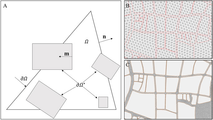
FIGURE 1. (A) Conceptual model of anisotropic porosity on a triangular grid, and examples of computational grids for. (B) porous shallow water modeling (PSWM) and (C) classical shallow water modeling (CSWM).

Accordingly, the volumetric porosity $\varphi$ that corresponds to the fraction of cell volume occupied by voids and the areal porosity $\psi$ that corresponds to the fraction of the plane occupied by voids are calculated by (Özgen et al., 2016)

$\varphi =\frac{{{\displaystyle \int }}_{\mathit{\Omega }}i\prime (\eta \prime -z_b)\text{d}\mathit{\Omega }}{{{\displaystyle \int }}_{\mathit{\Omega }}(\eta \prime -z_0)\text{d}\mathit{\Omega }},\psi =\frac{{{\displaystyle \mathrm{\oint }}}_{\partial \mathit{\Omega }}i\prime \left(\eta \prime -z_b\right)\text{d}r}{{{\displaystyle \mathrm{\oint }}}_{\partial \mathit{\Omega }}\left(\eta \prime -z_0\right)\text{d}r}$(6a, b)

where $z_0$ is the minimum bed elevation in the cell.

The interfacial term ${\mathbf{s}}^{\text{∗}}$ can be split into a stationary and a non-stationary components by (Sanders et al., 2008)

$\underset{\partial {\mathit{\Omega }}^{\text{∗}}}{{\displaystyle \mathrm{\oint }}}{\mathbf{s}}^{\ast }\text{d}{r}^{\text{∗}}=\underset{\partial {\mathit{\Omega }}^{\text{∗}}}{{\displaystyle \mathrm{\oint }}}\frac{1}{2}g{\left({h|}_{{\eta }_0}\right)}^2\mathbf{m\prime }\text{d}{r}^{\text{∗}}+\underset{\mathit{\Omega }}{{\displaystyle \int }}i\mathrm{\prime }{C}_D^b\mathbf{u\prime }V\text{d}\mathit{\Omega }(7)$

where the first and second terms on the right hand side of Eq. 7 are the stationary and non-stationary components, respectively; $\mathbf{m}=[m_x,m_y]$ is the unit normal vector along $\partial {\mathit{\Omega }}^{\text{∗}}$ with an inward direction toward the building and $\mathbf{m\prime }=[0,m_x,m_y]$; ${h|}_{{\eta }_0}$ is the hypothetical still water depth; $C_D^b$ is the drag coefficient related to the building effects; $\mathbf{u}=[u,v]$ is the velocity vector and $\mathbf{u\prime }=[0,u,v]$; $V=\sqrt{u^2+v^2}$. By substituting Eqs (6a,b) and Eq. 7 into Eq. 1, the integral form of the porous shallow water equations can be rewritten as

$\frac{\partial }{\partial t}\underset{\mathit{\Omega }}{{\displaystyle \int }}\varphi \mathbf{U}\text{d}\mathit{\Omega }+\underset{\partial \mathit{\Omega }}{{\displaystyle \mathrm{\oint }}}\psi \mathbf{En}\text{d}r=\underset{\mathit{\Omega }}{{\displaystyle \int }}\varphi \left(\mathbf{s}-C_D^b\mathbf{u\prime }V\right)\text{d}\mathit{\Omega }-\underset{\partial {\mathit{\Omega }}^{\text{∗}}}{{\displaystyle \mathrm{\oint }}}\frac{1}{2}g{\left({h|}_{{\eta }_0}\right)}^2\mathbf{m\prime }\text{d}{r}^{\text{∗}}(8)$

Numerical Methods

Based on the numerical methods in Hu et al. (2019), both of the porous and classical shallow water equations are solved under the framework of finite volume method using unstructured triangular grids. For simplicity, only the details for the porous shallow water model are elaborated.

Time Integration and Spatial Discretization

The time integration of Eq. 8 over $\text{Δ}t$ for cell $i$ reads

${\mathbf{U}}_i^{n+1}={\mathbf{U}}_i^n+\text{Δ}t\left({\mathbf{s}}_i-C_D^b\mathbf{u}{\mathrm{\prime }}_{\mathit{i}}{V}_i\right)+\frac{\text{Δ}t}{{\varphi }_i{A}_i}\left(-{\displaystyle \sum }_{j=1}^3{\psi }_j{\mathbf{E}}_{nj}\text{Δ}{r}_j-\underset{\partial {\mathit{\Omega }}^{\text{∗}}}{{\displaystyle \mathrm{\oint }}}\frac{1}{2}g{\left({h|}_{{\eta }_0}\right)}^2\mathbf{m\prime }\text{d}{r}^{\text{∗}}\right)(9)$

where ${\mathbf{U}}_i^n$ and ${\mathbf{U}}_i^{n+1}$ represent the vectors of conservative variables at time step $n$ and $n+1$, respectively; $\text{Δ}t$ is time step restrained by the Courant-Friendrichs-Lewy (CFL) condition with courant number of 0.45; The subscript $i$ and $j$ refer to cell $i$ and the $j$-th edge of cell $i$, respectively; $A_i$ is the area of cell $i$; $\text{Δ}{r}_j$ is the length of the $j$-th edge of cell $i$. Other variables and parameters are the same as the above unless otherwise specified.

Computation of Flux, Source Terms and Dry-Wet Fronts

For the computation of advection fluxes ${\mathbf{E}}_n$ at the interface of adjacent cells, the high-resolution Harten-Latex-van Leer-Contact (HLLC) approximate Riemann solver which is able to automatically capture shockwaves and discontinuities (Toro, 2001) is adopted. For the estimation of bed slope and friction, the slope flux method by Hou et al. (2013) and the splitting point-implicit method by Liang and Marche (2009) are used, respectively. The dry and wet cells are automatically judged and computed by the threshold water depth of $1\times {10}^{-6}$ m. Details are referred to Hu et al. (2019).

Computation of Interfacial Term ${\mathrm{s}}^{\ast }$

Stationary Component

For the stationary component (i.e., the last term on the right hand side (RHS) of Eq. 9), it is assumed that the hydrostatic fluid pressure along $\partial {\mathit{\Omega }}^{\text{∗}}$ is balanced by the bed slope and the hydrostatic fluid pressure along $\partial \mathit{\Omega }$ (Sanders et al., 2008). So we may write

$\underset{\partial {\mathit{\Omega }}^{\text{∗}}}{{\displaystyle \mathrm{\oint }}}\frac{1}{2}g{\left({h|}_{{\eta }_0}\right)}^2\mathbf{m\prime }\text{d}{r}^{\text{∗}}=-\underset{\partial \mathit{\Omega }}{{\displaystyle \mathrm{\oint }}}\frac{1}{2}g\psi {\left(h{|}_{{\eta }_0}\right)}^2\mathbf{n\prime }\text{d}r+\underset{\mathit{\Omega }}{{\displaystyle \int }}\varphi gh{|}_{{\eta }_0}\mathbf{s}{\mathrm{\prime }}_{\mathit{b}}\text{d}\mathit{\Omega }(10)$

where $\mathbf{n\prime }=[0,n_x,n_y]$ and $\mathbf{s}{\mathrm{\prime }}_{\mathit{b}}=[0,s_{bx},s_{by}]$. The hydrostatic fluid pressure along $\partial \mathit{\Omega }$ in Eq. 10 can be evaluated by

$\underset{\partial \mathit{\Omega }}{{\displaystyle \mathrm{\oint }}}\frac{1}{2}g\psi {\left(h{|}_{{\eta }_0}\right)}^2\mathbf{n\prime }\text{d}r={\displaystyle \sum }_{j=1}^3\frac{1}{2}\left(g{\psi }_j{h}_j^2\mathbf{n}{\mathrm{\prime }}_{\mathit{j}}\text{Δ}{r}_j\right)(11)$

where $h_j$ is the water depth at the mid-point of the $j$-th edge of cell $i$, which is estimated by Eq. 12 in order to ensure non-negative value (Audusse et al., 2004).

$h_j=\max \left(0,{\eta }_{0i}-Z_{bj}\right)(12)$

where ${\eta }_{0i}$ is the static water level approximated by the water level at the cell center; $Z_{bj}$ is the maximum bed elevation of the two cell centers located on the two sides of the interface $j$. The discretization of the bed slope term in Eq. 10 follows the slope flux method by Hou et al. (2013),

$\underset{\mathit{\Omega }}{{\displaystyle \int }}\varphi gh{|}_{{\eta }_0}\mathbf{s}{\mathrm{\prime }}_{\mathit{b}}\text{d}\mathit{\Omega }=-{\displaystyle \sum }_{j=1}^3\frac{1}{2}g\varphi \mathbf{n}{\mathrm{\prime }}_{\mathit{j}}\left(h_i+h_j\right)\left({\overline{Z}}_{bj}-Z_{bi}\right)\text{Δ}{r}_j(13)$

where $h_i$ and $Z_{bi}$ is the water depth and bed elevation at the cell center; ${\overline{Z}}_{bj}=\text{min}(Z_{bj},{\eta }_{0i})$.

Non-Stationary Component

For the non-stationary component, the approach used for vegetation resistance modeling (Nepf, 1999) is extended to estimate the building drag force. Considering the anisotropy property, the non-starionary building drag force per unit area can be written as

$C_D^b\mathbf{u}{\mathrm{\prime }}_{\mathit{i}}{V}_i=\frac{1}{2{\varphi }_i{A}_i}{\displaystyle \sum }_{k=1,K}{C}_{Dk}^0{h}_i{\mathbf{E}}_{uk}{V}_i(14)$

where $K$ is the number of building edges in a cell; the subscript $i$ is the cell index, the subscript $k$ is the building edge index; $C_{Dk}^0$ is the drag force coefficient of the $k$–th building edge; ${\mathbf{E}}_{uk}=\left[0,l_k{m}_{x}u,l_k{m}_{y}v\right]$; $l_k$ is the length of the $k$–th building edge. In case the building edge is in the sheltered back face of the building, $C_{Dk}^0$ is set to zero. Other variables are the same as specified above.

Estimation of Infiltration Effects

The infiltration processes of the land surface are described by the Horton′s method (Akan, 1992), which is

$f_{p,t}=\{\begin{array}{l}{f}_{\infty }+\left(f_0-f_{\infty }\right)e^{-k_{d}t}\mathit{if}F\left(t\right)\mathrm{\prime }=F\left(t\right)\\ f_0\mathit{if}F\left(t\right)\mathrm{\prime }>F\left(t\right)\end{array}(15)$

$f\left(t\right)=\text{min}\left(f_{p,t},q+h/\text{Δ}t\right)(16)$

where $f_{p,t}$ is the infiltration capacity at time $t$ by the Horton′s method; $f_0$ and $f_{\infty }$ are the infiltration capacity at $t$ = 0 and for the saturated status, respectively; $k_d$ is the decaying rate of the infiltration capacity; $f\left(t\right)$ is the actual infiltration rate at time $t$; $F{\left(t\right)}^{\prime }=\underset{0}{\overset{t}{{\displaystyle \int }}}{f}_{\infty }+\left(f_0-f_{\infty }\right)e^{-k_{d}t}\text{d}t$ is the total infiltration amount till time $t$ following the Horton′s method; $F\left(t\right)=\underset{0}{\overset{t}{{\displaystyle \int }}}f\left(t\right)\text{d}t$ is the actual total infiltration amount till time $t$. Other parameters are the same as specified above.

Study Areas

The Zhoushan archipelago, which is composed of thousand islands, is located at the conjunction of the Yangtze River Estuary and Hangzhou Bay in the East China Sea (Figure 2A). The Zhoushan city is in the main island of the archipelago, which has an area of 468.7 km² and is the fourth biggest island in China. Under the influences of subtropical marine monsoon climate, storms and typhoons occur frequently in summer and autumn and cause heavy rainfall in this area. The rainfall is mostly concentrated in the south-western region (Dinghai district) where the city center is located.

FIGURE 2

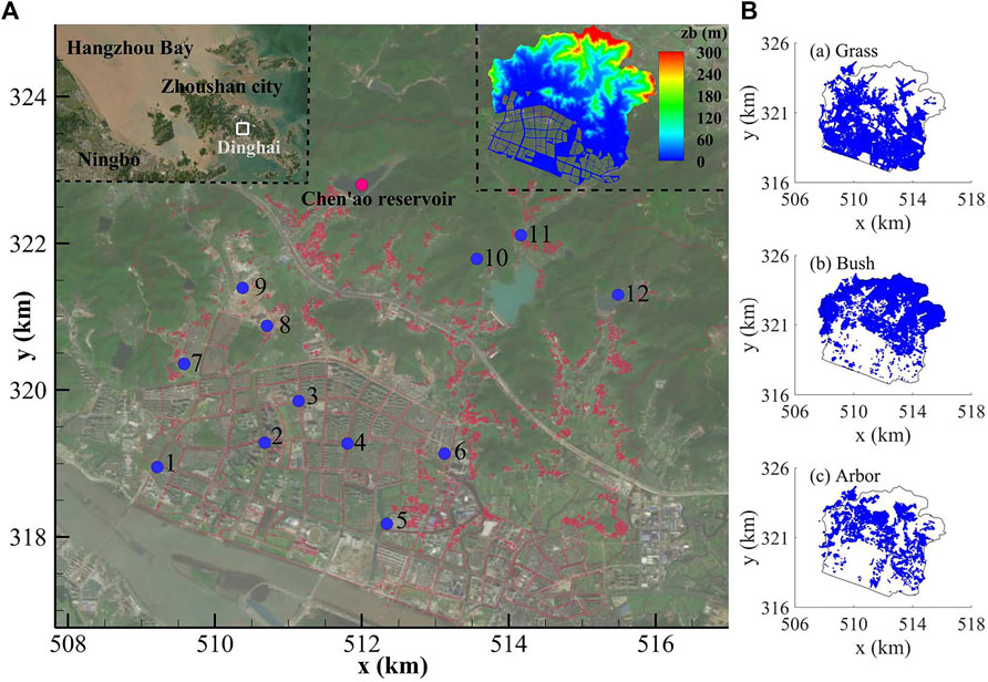
FIGURE 2. (A) Study area, topography and selected points (B) vegetation types.

In the period of 1960–2009, there are 187 typhoon events that have affected Zhoushan and 52 events (27.8%) induce heavy rainfall (e.g., daily rainfall >50 mm) (Wang et al., 2011). Based on the historical data, there are 42 and 15 events characterized by the total rainfall higher than 100 and 200 mm, respectively. In the past 2 decades, the typhoon-induced rainstorm is intensified in both frequency and magnitude due to the global warming. Moreover, the lack of big rivers to accommodate strong rainfall flow and the dramatic increase of impermeable surface due to rapid urbanization aggravate the urban flood risks. Consequently, large areas of farmlands and urban districts are inundated frequently during typhoon-induced rainstorms. In addition, the extreme rainfall may also cause flash floods, landslides and debris flow in the mountainous areas. These result in catastrophic destroy in infrastructures, ecology, environment, social economy and even death.

In the present simulation, we focus on the rainfall-induced surface runoff in a catchment of Dinghai district (Figure 2A). The catchment is 46.28 km² with a perimeter of about 31.3 km, where dense urban areas and mountains are included.

Model Set-Up

Rainfall Processes

We consider the rainfall processes when the super Typhoon Lekima passed the Zhoushan City from August 9^th to 11^th in 2019. The variation of rainfall intensity per hour at the Chen′ao Reservoir (Figure 2A) is shown in Figure 3, for which the data is available online at http://www.zjsq.net.cn:8010/webwarn/. The rainfall mainly occurs in the first 30 h featured by a strong unsteady and undulated pattern. The maximum rainfall intensity is 41 mm/h at 14 h. As no more rainfall data is open-access for this catchment, we assume the rainfall is evenly distributed in space and the rainfall process at the Chen′ao Reservoir is used for all computational cells.

FIGURE 3

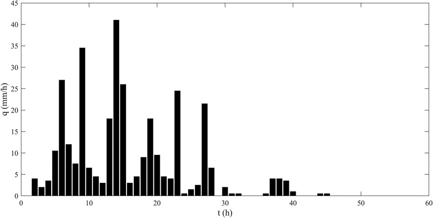
FIGURE 3. Rainfall intensity at the Chen’ao Reservoir during the Typhoon Lekima.

Building Treatment

In the catchment, different building treatments are employed for the dense urban areas and the isolated houses, respectively. The former is composed of many residential units bounded by streets or borders (e.g., relatively large red polygons in the lower part of Figure 2A). Due to the lack of high resolution data for the details inside the residential units, we consider each residential unit as an integral by neglecting the detailed information of buildings. In comparison, the latter is characterized by a much smaller size and scattered distributions (e.g., small red dots in Figure 2A). The impacts of an individual house on the hydrodynamic processes are spatial and temporal limited, so we make a simplification for saving the computational costs. For an isolated house with an area larger than 3,000 m², we consider its effects by describing its border through polygons. Otherwise, the effects of isolated houses are neglected.

Infiltration Effects of Different Vegetation Types

The infiltration effects of the underlying surface are determined by many factors, such as vegetation types, soil properties, and rainfall intensity etc. (Cen et al., 1997; Liu et al., 2014; Fernández-Pato et al., 2016; Xing et al., 2019). Here, we focus on the vegetation-related infiltration effects. There is a diversity of vegetation in the catchment including grass, crops, vegetables and trees like poplar, bayberry and grapefruit, etc. In the modeling, we categorize them into three types by grass, bush and arbor, respectively. Their spatial distributions are illustrated in Figure 2B.

According to Tao et al. (2017), the influences of different vegetation on the infiltration processes are manifested by the infiltration capacity $\left(f_0,f_{\infty }\right)$ and the decaying rate $k_d$ (Table 1). For each computational cell, the parameters of the comprehensive infiltration capacity and the decaying rate are the weighted average of each vegetation type based on the distribution density of each vegetation in the cell.

TABLE 1

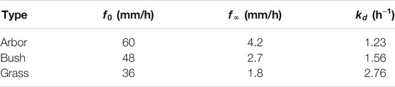
TABLE 1. Infiltration parameters of different vegetation.

Numerical Cases, Grids and Parameters

Three cases are designed to investigate the pros and cons of the porosity model and the infiltration effects on the modeling results. Case 1 is the reference case using the porous shallow water modeling (PSWM) without infiltration effects. Its comparison with Case 2 using classical shallow water modeling (CSWM) shows the magnitude of accuracy and efficiency of the porosity method. Case 3 is similar to Case 1 but with infiltration effects.

As shown in Figures 1B,C, the CSWM directly excludes the buildings from the computational domain and refines the grids around the buildings. This is the most delicate way to model the surface water flow along the streets. Yet, it is also time consuming for large-scale simulation. To save the computational cost while maintaining adequate accuracy, the PSWM uses relatively coarse grids to simulate the surface water flow while the building effects of storage and conveyance are considered by the volumetric and areal porosity parameters. Thus, the water flowing area of a coarse grid in the porosity model is equivalent to a random polygon bounded by the edges of the grid and the buildings inside. In this case, for the grids which are entirely inside the building areas, no computation is done; only for the grids which cover the streets (some grids may include small parts of the buildings), the computation is conducted. The total water flowing areas in the two models are therefore the same though the total areas of the effective computational domains in the two models have some differences due to the imperfect overlap of the edges of buildings and coarse grids. In the simulation, the total grid number for PSWM (Cases 1 and 3) is 22,397 with the grid size ranging from 43 to 82 m; it is 161,665 for CSWM (Case 2) with the grid size between 12 and 30 m.

Along the borders of the catchment, the free-outflow boundary condition is implemented. As no big rivers in the catchment, we neglect the river channels for simplicity while the reservoirs in the mountains are reserved. The pluvial flood is initiated by the rainfall of the Typhoon Lekima on an initially dry bed and the simulation lasts for 66 h. Actually, the Manning roughness coefficient $n$ in estimating the bed friction effects (Eq. 3a, b) may be varied for different land surfaces, e.g., the road made of concrete may have different roughness from the vegetated areas. However, for the real urban flood modeling, the Manning roughness coefficient is usually set as constant to avoid uncertainties raising from the empirical value setting for different land surface materials (Schubert and Sanders, 2012; Kim et al., 2014; Sanders and Schubert, 2019). Thus, we use a constant Manning roughness coefficient $n=0.02$ for both PSWM and CSWM. The empirical parameter $C_{Dk}^0$ for estimating the drag force is usually considered as a constant (Sanders et al., 2008; Schubert and Sanders, 2012; Kim et al., 2014; Guinot et al., 2017). Its value ranges between 0 and 2 for different experiments and field-scale simulations, and there have been no consensus on which value is more appropriate. In the present modeling, the effects of different buildings on the drag force are accounted for by the vector ${\mathbf{E}}_{uk}$ in Eq. 14 while the empirical parameter $C_{Dk}^0$ is assumed to be two based on the suggestions by Munson et al. (2006) for square forms in 2D flows. Extra tests (not shown) also indicate that the computed water depth and velocity in PSWM are not so sensitive with different values of $C_{Dk}^0$ (e.g., 0, 1, 2), but they show better agreement with CSWM in dense urban areas when $C_{Dk}^0=$ 2 is used. All the simulations are carried out using 12 cores of the Intel(R) Xeon(R) Platinum 8173M CPU @ 2.00 GHz processor.

Model Results

Comparison Between PSWM and CSWM

For the simulation of 66 h pluvial flood in the concerned catchment, the wall clock time of the CSWM and PSWM is 17154 and 120 min, respectively. It indicates that the porosity method may speed up the simulation by about 143 times saving 99% of the computational time. The computations of the two models generally agree with each other quite well, but discrepancies in specific locations are still visible. The spatial and temporal properties of water depth and flow velocity and their comparisons between the two models are shown as following.

Water Depth

The spatial distributions of water depth are qualitatively the same in the two models (Figures 4, 5). Among the most parts of the mountains, the water depth is the lowest. The surface shallow flow runs downward along hillslopes resulting in deeper water in the valleys. The three reservoirs in the mountains retaining the rainfall and surface runoff show a large water depth. At the interface of the mountains and the urbanized areas, the water depth shows a remarkable increase possibly due to the blocking effects of the residential units and the sudden decrease of bed slope. This is exemplified by the large water depth just outside the urbanized areas at the foot of the mountains (e.g., yellow and red parts on the left of Figures 4, 5). In addition, the lowland areas without significant urbanization also show an obvious retaining effect on the rainfall and surface flows (e.g., light blue and green parts on the right of Figures 4, 5). Among the residential units, the water depth along the streets is mostly between those in the valleys and lowland areas. The differences of water depth among those streets depend on the width and directions of the streets, arrangements of the residential units, and changes of land-surface elevation, etc.

FIGURE 4

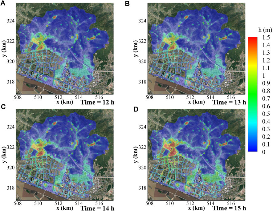
FIGURE 4. Temporal and spatial evolution of water depth for PSWM in Case 1 at (A) 12 h, (B) 13 h, (C) 14 h and (D) 15 h.

FIGURE 5

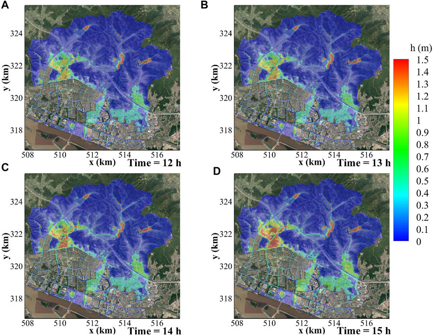
FIGURE 5. Temporal and spatial evolution of water depth for CSWM in Case 2 at (A) 12 h, (B) 13 h, (C) 14 h and (D) 15 h.

For the time evolution of the surface flow, the water depth shows an increasing trend with the enhancement of rainfall intensity (Figures 4, 5). Note that there exists a time lag between the rainfall peak ($t=14$ h) and the maximum water depth ($t=15$ h) in the catchment (see Figures 3–5). This is mainly because that it takes time for the surface runoff to accumulate and the change of water depth could be delayed. Furthermore, Figure 6 illustrates the magnitudes of water depth increase from 12 to 15 h for the two models showing similar trends. The largest depth increase during the rainfall processes is in the streets of the dense urban areas especially for those near the main path connecting the interface (e.g., red color in Figure 6). In addition, the interface area that is featured by deep water (e.g., orange color on the left of Figure 6) and the partly-blocked low-lying areas (e.g., yellow-green color on the right of Figure 6) also show a remarkable increase. In the mountainous areas the depth increase is rather small (e.g., dark blue in Figure 6) except for the reservoirs.

FIGURE 6

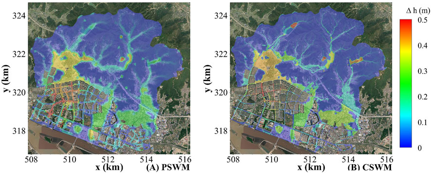
FIGURE 6. Spatial distribution of depth increase from 12 to 15 h for. (A) PSWM and (B) CSWM.

To get a further insight into the details of the two models, some discrepancies are still existed (Figures 4, 5). On the mountainous areas, the calculated water depth in the PSWM is not as smooth as that in the CSWM. For the former, small puddles are scattered in this area mainly due to the low resolution of the complex topography (e.g., locally steep slopes and delicate undulations) when using large grids. In the dense urban areas, the flow width and depth along the streets are a bit larger in the PSWM. This is probably related to the imperfect overlap of the grids and borders of the residential units when using large grids and the approximation errors at extremely low porosity locations (Figure 1B).

As the observational data are not easily available, we select 12 points (Figure 2A) to examine the model performance in different region types. Points 1–4 lie in the dense urban areas to represent the street flow, Points 5-6 at low-lying areas partly surrounded by isolated houses and residential units, Points 7–9 at the interface between mountains and urbanized regions, and Points 10–12 in the mountainous areas. The computed water depth variations show distinct characteristics among different regional types (Figure 7). For the highland areas (e.g., P10 and P11), the surface flow is directly determined by the rainfall intensity, so the dry bed becomes wet immediately after it starts raining. The surface water is shallow with remarkable depth fluctuations in response to the sharp changes of rainfall intensity. For other low-lying areas (e.g., other points), the water depth is affected by both rainfall intensity and the convergence of surface flow, so there is a delay for the depth increase and the maximum depth is much larger. Though sharp increase of water depth is also observed, the temporal variation is much smoother compared to that in the highlands. For the comparison of the two models, good agreement is achieved at most points though visible discrepancies are still existed in streets between residential units (e.g., P1-P3) and steep-sloped hills (e.g., P11) due to the complex layouts and geometries of buildings and the low grid resolution for steep slopes.

FIGURE 7

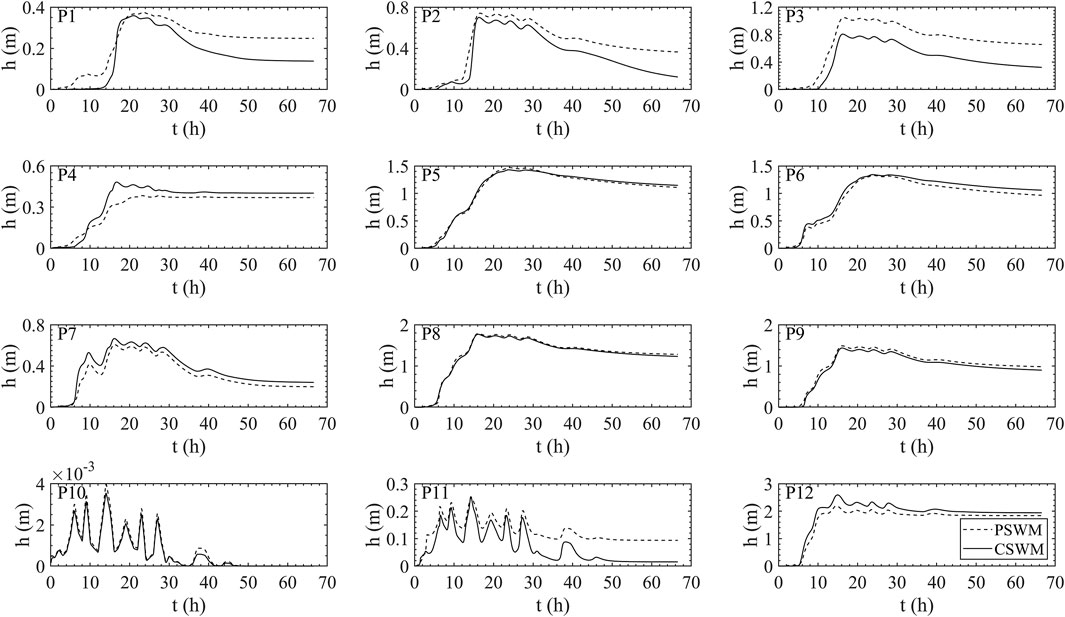
FIGURE 7. Temporal evolution of water depth at 12 selected points for PSWM and CSWM.

Velocity

Though the velocity computation of PSWM has a lower resolution compared to that of CSWM, the general trends of the two models are very similar (Compared Figure 8 with Figure 9). In the mountainous areas, low velocity occurs on the hillslopes where the surface flow is very shallow. Due to the accumulation of surface flow in the valleys, the flow energy is strengthened and the velocity becomes higher. This results in that the maximum flow velocity is distributed along those valleys. Along the interface of the mountains and the urbanized areas, the velocity depends on the blocking extent and flow mobility. Under strong blocking effects, large amount of water is retained locally and the flow is decelerated dramatically (e.g., the low velocity area with deepest water on the left of Figures 8, 9). In case there is other space available for the flow routing, for example, moving along the interface, the velocity might be as high as that in the valleys. Inside the urbanized areas, the velocity along streets could be similar or even higher than that at the interface. Its spatial distribution depends on the width and directions of the streets, alignments of residential units and bed elevations, etc. In general, the streets featuring deeper water show higher velocity, which bears similarity to valleys. Like the evolution of water depth, the flow velocity in the catchment is also increased with rainfall intensity but characterized by a delayed response.

FIGURE 8

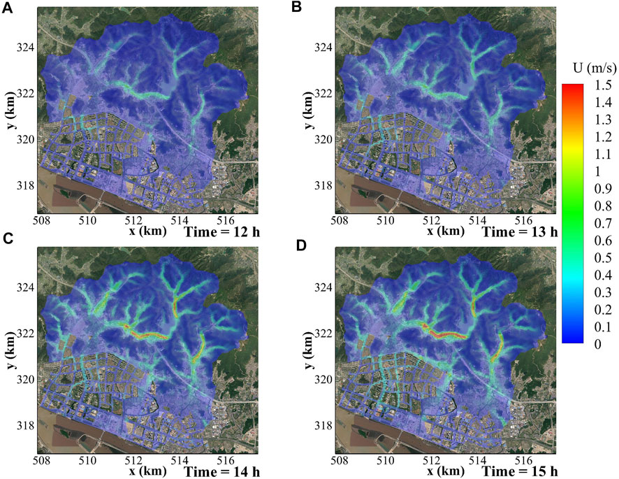
FIGURE 8. Temporal and spatial evolution of flow velocity for PSWM in Case 1 at (A) 12 h, (B) 13 h, (C) 14 h and (D) 15 h.

FIGURE 9

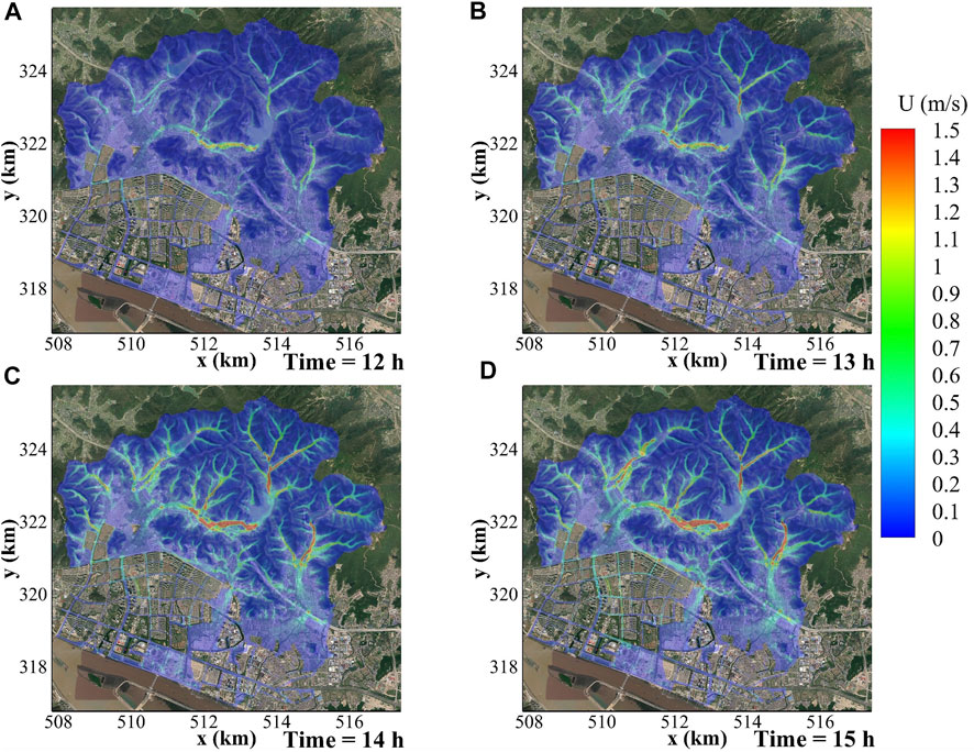
FIGURE 9. Temporal and spatial evolution of flow velocity for CSWM in Case 2 at (A) 12 h, (B) 13 h, (C) 14 h and (D) 15 h.

At the specific points, the flow velocity is more sensitive to the rainfall intensity than water depth (Figure 10). It is shown by the strong fluctuations of velocity with relatively large magnitude at heavy rainfalls and a smooth trend with small magnitude at light rainfalls (e.g., after 30 h). The velocity could be very small either in very shallow waters (e.g., P1, P4, P10) or in the retained deep waters (e.g., P5, P8, P12). Besides, the magnitude of velocity is also largely affected by local topography. For instance, a steep slope may introduce large flow velocity in shallow waters (e.g., P11). In general, the computed velocity of the two models (Figure 10) is in line with each other. However, because the velocity computation has a higher requirement on the grid resolution, the velocity differences of the two models are a bit larger than the water depth.

FIGURE 10

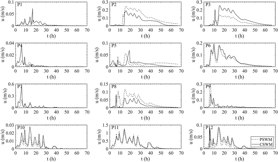
FIGURE 10. Temporal evolution of flow velocity at 12 selected points for PSWM and CSWM.

To further compare the direction and magnitude of velocity computation in the two models, the spatial distributions of velocity vectors at $t=14$ h are shown in Figure 11 (red refers to PSWM, black refers to CSWM). Along the streets in the residential units (Figure 11A) and around the isolated houses (Figure 11B), the vectors are generally in good agreements. This implies that the PSWM could adequately capture the main features of flow movement in such areas dominated by the interactions of buildings and streets. In addition, the vectors in the mountains also agree well between the two models (Figure 11C) showing acceptable accuracy of PSWM with large grids in the steep-sloped mountainous areas.

FIGURE 11

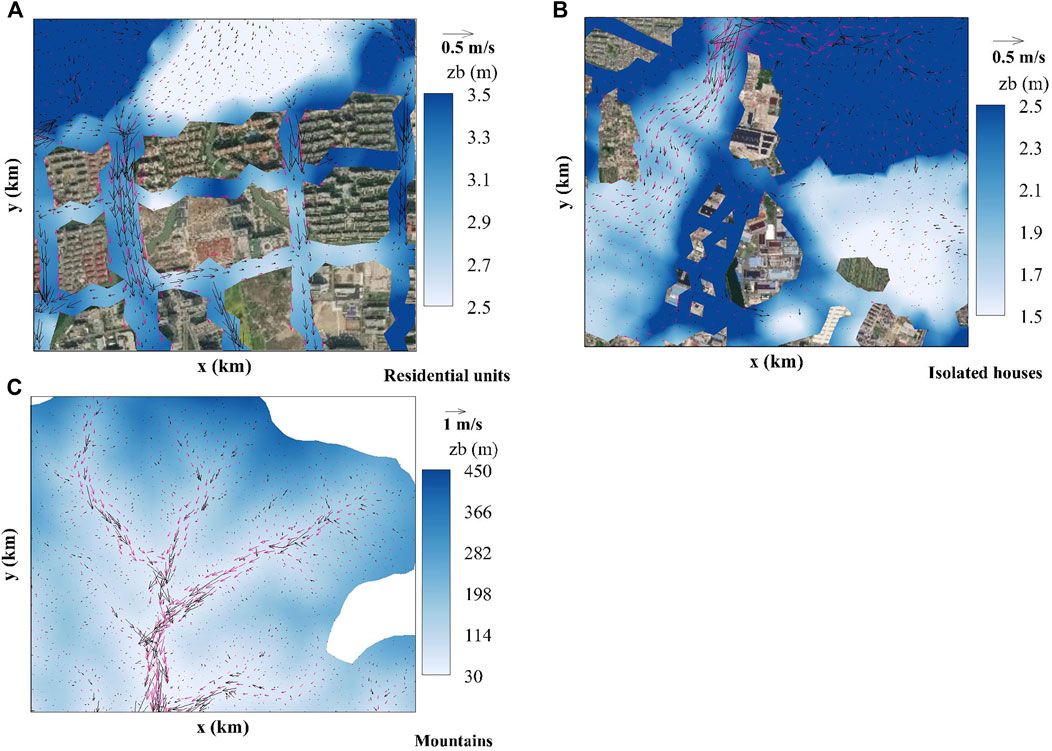
FIGURE 11. Comparison of velocity vectors of the two models in. (A) residential units. (B) isolated houses, and (C) mountains.

Impacts of Land Surface Infiltration

The impacts of land surface infiltration are investigated for PSWM by the comparison of Cases 1 (no infiltration) and 3 (with infiltration). The temporal evolution and spatial distribution of depth and velocity are almost unchanged when the infiltration effects are considered, whereas both magnitudes reduce markedly as shown by the computed results at $t=$ 15 h in Figure 12.

FIGURE 12

FIGURE 12. (A) Water depth and (B) flow velocity at $t=$ 15 h for PSWM with infiltration in Case 3.

Figure 13 shows the reduction in magnitude and percentage for depth, respectively. On the aspect of magnitude, the largest reduction is observed in the areas of relatively large water depth, shown by dark blue (i.e., the interface between mountains and urbanized areas, and the wide streets connecting the main path to the interface) on the left of Figure 13A. In terms of percentage, the most significant reduction occurs mainly in the streets of the dense urban areas (Figure 13B). These findings are inconsistent with the spatial distribution of vegetation types. According to the spatial distribution, the vegetation on the mountains is dominated by bush and anchor (Figure 2B), which have relatively large infiltration capacities, and thus the reduction directly related to infiltration should be larger than that in the urbanized areas where grass is dominant. However, the largest reduction is in the grass-dominated areas. This implies that the infiltration processes not only have a local effect based on the vegetation type, but also extend its spatial influences through surface flow networking. The surface flow in the urbanized areas may have two sources: one is the rainfall, the other is the converging water flow from the mountainous areas. Yet the relatively strong infiltration on the mountains causes less surface flow to go downward to the mountain-city interface and the streets inside, so the convergence contribution is reduced. In case the role of converging flow reduction exceeds that of the infiltration differences between different vegetation types (e.g., between grass and bush/arbor), the water depth decrease could be considerable and this might be the reason for the largest reduction in the urbanized areas.

FIGURE 13

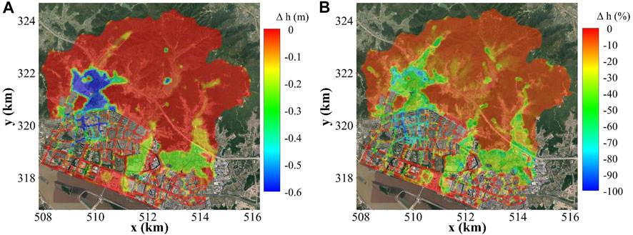
FIGURE 13. Reduction of water depth by infiltration in. (A) magnitude and (B) percentage.

Figure 14 shows the comparison of temporal variations of water depth at the specific points for Cases 1 and 3. By considering the infiltration effects in Case 3, a delay is observed for the start of water depth increase (i.e., land surface from dry to wet) at all points when compared to Case 1 without infiltration. This delay is the longest in the mountainous areas (e.g., P10 and P11) and the shortest in the streets of urbanized areas (e.g., P1-P4). Other places are in-between (e.g., P5-P9). Regarding the reduction magnitude, the infiltration is mainly effective during the high rainfall intensity periods before $t=30$ h. After that the difference of water depth with and without infiltration becomes minor. For the flow velocity, the time lag is also existed at all points for Case 3 with infiltration. However, except for the obvious velocity decrease in the streets near the main path areas connecting the interface, other places do not show a universe infiltration effect on flow velocity.

FIGURE 14

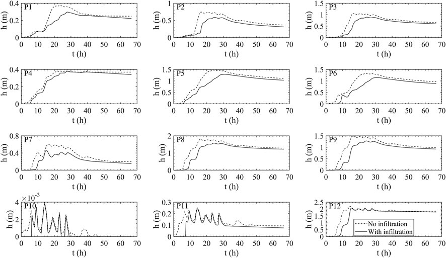
FIGURE 14. Temporal evolution of water depth at 12 selected points for PSWM with and without infiltration.

Conclusion

Two models (i.e., the classical shallow water model and the porous shallow water model) have been developed and compared for urban flood modeling in the city of Zhoushan (China). The pluvial flooding induced by the super Typhoon Lekima in 2019 in a 46 km² mountain-bounded urban area is simulated. The main conclusions include:

The computation of water depth and flow velocity of the two models agree with each other quite well. It is shown that the largest water depth is prone to occur in the interface between mountains and dense urban areas where surface flow is dramatically decelerated by building blocking and abrupt flattening in terrains. Moreover, the streets in urban areas connecting the main paths to the interface and the partly-blocked low-lying regions may also encounter large water depth. The highest flow velocity occurs in the steep-sloped valleys among mountains due to the surface flow converging from surrounding hillslopes.

The infiltration processes not only have a local effect based on the vegetation type, but also extend its spatial influences through surface flow networking. Thus, the magnitude of water depth reduction may not be consistent with the infiltration capacity of vegetation if the networking effect is stronger than the infiltration difference related to local vegetation type.

For a 2.8 days prediction, the computational cost is 120 min for the porous shallow water model using 12 cores of the Intel(R) Xeon(R) Platinum 8173 M CPU @ 2.00 GHz processor, whereas it is as high as 17,154 min for the classical shallow water model. It indicates a speed-up of 143 times and sufficient pre-warning time by using the porous shallow water model, without appreciable loss in the quantitative accuracy.

Data Availability Statement

The original contributions presented in the study are included in the article/supplementary material, further inquiries can be directed to the corresponding author.

Author Contributions

WL contributed to the idea initiation, result analysis, article writing and supervised BL to develop the porous shallow water model. BL developed the porous shallow water model and did the simulations. PH contributed to the idea initiation and result analysis. ZH contributed to the result analysis. JZ prepared the rainfall, topography and vegetation data. All authors contributed to the article and approved the submitted version.

Funding

This research is sponsored by the National Natural Science Foundation of China (No. 11872332, 11772300), the Zhejiang Natural Science Foundation (LR19E090002).This research is supported by the HPC Center of ZJU (ZHOUSHAN CAMPUS).

Conflict of Interest

The authors declare that the research was conducted in the absence of any commercial or financial relationships that could be construed as a potential conflict of interest.

References

Akan, A. O. (1992). Horton infiltration equation revisited. J. Irrigation Drainage Eng. 118, 828–830. doi:10.1061/(ASCE)0733-9437

CrossRef Full Text | Google Scholar

Audusse, E., Bouchut, F., Bristeau, M.-O., Klein, R., and Perthame, B. (2004). A fast and stable well-balanced scheme with hydrostatic reconstruction for shallow water flows. SIAM J. Sci. Comput. 25, 2050–2065. doi:10.1137/S1064827503431090

CrossRef Full Text | Google Scholar

Bellos, V., and Tsakiris, G. (2016). A hybrid method for flood simulation in small catchments combining hydrodynamic and hydrological techniques. J. Hydrol. 540, 331–339. doi:10.1016/j.jhydrol.2016.06.040

CrossRef Full Text | Google Scholar

Brown, J. D., Spencer, T., and Moeller, I. (2007). Modeling storm surge flooding of an urban area with particular reference to modeling uncertainties: a case study of Canvey Island, United Kingdom. Water Resour. Res. 43, 1–22. doi:10.1029/2005WR004597

PubMed Abstract | CrossRef Full Text | Google Scholar

Cea, L., and Vázquez-Cendón, M. E. (2010). Unstructured finite volume discretization of two-dimensional depth-averaged shallow water equations with porosity. Int. J. Numer. Meth. Fluids. 63, 903–930. doi:10.1002/fld.2107

CrossRef Full Text | Google Scholar

Cen, G., Shen, J., Fan, R., and Wang, Y. (1997). Experimental study on urban surface runoff yield. J. Hydraulic Eng., 48–53+72. (in Chinese).

Google Scholar

Chen, A. S., Evans, B., Djordjević, S., and Savić, D. A. (2012). Multi-layered coarse grid modelling in 2D urban flood simulations. J. Hydrol. 470-471, 1–11. doi:10.1016/j.jhydrol.2012.06.022

CrossRef Full Text | Google Scholar

Cheng, T., Xu, Z., Yang, H., Hong, S., and Leitao, J. P. (2020). Analysis of effect of rainfall patterns on urban flood process by coupled hydrological and hydrodynamic modeling. J. Hydrol. Eng. 25, 04019061. doi:10.1061/(ASCE)HE.1943-5584.0001867

CrossRef Full Text | Google Scholar

Costabile, P., Costanzo, C., and Macchione, F. (2017). Performances and limitations of the diffusive approximation of the 2-d shallow water equations for flood simulation in urban and rural areas. Appl. Numer. Math. 116, 141–156. doi:10.1016/j.apnum.2016.07.003

CrossRef Full Text | Google Scholar

Defina, A. (2000). Two-dimensional shallow flow equations for partially dry areas. Water Resour. Res. 36, 3251–3264. doi:10.1029/2000WR900167

CrossRef Full Text | Google Scholar

Fernández-Pato, J., Caviedes-Voullième, D., and García-Navarro, P. (2016). Rainfall/runoff simulation with 2D full shallow water equations: sensitivity analysis and calibration of infiltration parameters. J. Hydrol. 536, 496–513. doi:10.1016/j.jhydrol.2016.03.021

CrossRef Full Text | Google Scholar

Gross, M. (2016). The urbanisation of our species. Curr. Biol. 26, R1205–R1208. doi:10.1016/j.cub.2016.11.039

PubMed Abstract | CrossRef Full Text | Google Scholar

Guinot, V., Sanders, B. F., and Schubert, J. E. (2017). Dual integral porosity shallow water model for urban flood modelling. Adv. Water Resour. 103, 16–31. doi:10.1016/j.advwatres.2017.02.009

CrossRef Full Text | Google Scholar

Guinot, V., and Soares-Frazão, S. (2006). Flux and source term discretization in two-dimensional shallow water models with porosity on unstructured grids. Int. J. Numer. Meth. Fluids 50, 309–345. doi:10.1002/fld.1059

CrossRef Full Text | Google Scholar

Hou, J., Liang, Q., Simons, F., and Hinkelmann, R. (2013). A 2D well-balanced shallow flow model for unstructured grids with novel slope source term treatment. Adv. Water Resour. 52, 107–131. doi:10.1016/j.advwatres.2012.08.003

CrossRef Full Text | Google Scholar

Hu, P., Lei, Y., Han, J., Cao, Z., Liu, H., and He, Z. (2019). Computationally efficient modeling of hydro-sediment-morphodynamic processes using a hybrid local time step/global maximum time step. Adv. Water Resour. 127, 26–38. doi:10.1016/j.advwatres.2019.03.006

CrossRef Full Text | Google Scholar

Huang, Q., Wang, J., Li, M., Fei, M., and Dong, J. (2017). Modeling the influence of urbanization on urban pluvial flooding: a scenario-based case study in Shanghai, China. Nat. Hazards. 87, 1035–1055. doi:10.1007/s11069-017-2808-4

CrossRef Full Text | Google Scholar

Hunter, N. M., Bates, P. D., Neelz, S., Pender, G., Villanueva, I., Wright, N. G., et al. (2008). Benchmarking 2D hydraulic models for urban flooding. Proc. Inst. Civil Eng. - Water Manag. 161, 13–30. doi:10.1680/wama.2008.161.1.13

CrossRef Full Text | Google Scholar

IPCC (2014). Climate Change 2014: impacts, adaptation and vulnerability: part A: global and section aspects. United Kingdom: Cambridge University Press.

Kim, B., Sanders, B. F., Famiglietti, J. S., and Guinot, V. (2015). Urban flood modeling with porous shallow-water equations: a case study of model errors in the presence of anisotropic porosity. J. Hydrol. 523, 680–692. doi:10.1016/j.jhydrol.2015.01.059

CrossRef Full Text | Google Scholar

Kim, B., Sanders, B. F., Schubert, J. E., and Famiglietti, J. S. (2014). Mesh type tradeoffs in 2D hydrodynamic modeling of flooding with a Godunov-based flow solver. Adv. Water Resour. 68, 42–61. doi:10.1016/j.advwatres.2014.02.013

CrossRef Full Text | Google Scholar

Kreibich, H., Thaler, T., Glade, T., and Molinari, D. (2019). Preface: damage of natural hazards: assessment and mitigation. Nat. Hazards Earth Syst. Sci. 19, 551–554. doi:10.5194/nhess-19-551-2019

CrossRef Full Text | Google Scholar

Leandro, J., Chen, A. S., and Schumann, A. (2014). A 2D parallel diffusive wave model for floodplain inundation with variable time step (P-DWave). J. Hydrol. 517, 250–259. doi:10.1016/j.jhydrol.2014.05.020

CrossRef Full Text | Google Scholar

Leandro, J., Schumann, A., and Pfister, A. (2016). A step towards considering the spatial heterogeneity of urban key features in urban hydrology flood modelling. J. Hydrol. 535, 356–365. doi:10.1016/j.jhydrol.2016.01.060

CrossRef Full Text | Google Scholar

Liang, Q., and Marche, F. (2009). Numerical resolution of well-balanced shallow water equations with complex source terms. Adv. Water Resour. 32, 873–884. doi:10.1016/j.advwatres.2009.02.010

CrossRef Full Text | Google Scholar

Liu, J., Shao, W., Xiang, C., Mei, C., and Li, Z. (2020). Uncertainties of urban flood modeling: Influence of parameters for different underlying surfaces. Environ. Res. 182, 108929. doi:10.1016/j.envres.2019.108929

PubMed Abstract | CrossRef Full Text | Google Scholar

Liu, L., Liu, Y., Wang, X., Yu, D., Liu, K., Huang, H., et al. (2015). Developing an effective 2-D urban flood inundation model for city emergency management based on cellular automata. Nat. Hazards Earth Syst. Sci. 15, 381–391. doi:10.5194/nhess-15-381-2015

CrossRef Full Text | Google Scholar

Liu, W., Chen, W., and Peng, C. (2014). Assessing the effectiveness of green infrastructures on urban flooding reduction: a community scale study. Ecol. Model. 291, 6–14. doi:10.1016/j.ecolmodel.2014.07.012

CrossRef Full Text | Google Scholar

Löwe, R., Urich, C., Sto. Domingo, N., Mark, O., Deletic, A., and Arnbjerg-Nielsen, K. (2017). Assessment of urban pluvial flood risk and efficiency of adaptation options through simulations - A new generation of urban planning tools. J. Hydrol. 550, 355–367. doi:10.1016/j.jhydrol.2017.05.009

CrossRef Full Text | Google Scholar

Min, S.-K., Zhang, X., Zwiers, F. W., and Hegerl, G. C. (2011). Human contribution to more-intense precipitation extremes. Nature 470, 378–381. doi:10.1038/nature09763

PubMed Abstract | CrossRef Full Text | Google Scholar

Munson, B., Young, D., and Okiishi, T. (2006). Fundamentals of fluid mechanics. fifth ed. New York: John Wiley & Sons.

Neal, J., Villanueva, I., Wright, N., Willis, T., Fewtrell, T., and Bates, P. (2012). How much physical complexity is needed to model flood inundation? Hydrol. Process. 26, 2264–2282. doi:10.1002/hyp.8339

CrossRef Full Text | Google Scholar

Nepf, H. M. (1999). Drag, turbulence, and diffusion in flow through emergent vegetation. Water Resour. Res. 35, 479–489. doi:10.1029/1998WR900069

CrossRef Full Text | Google Scholar

Özgen, I., Zhao, J., Liang, D., and Hinkelmann, R. (2016). Urban flood modeling using shallow water equations with depth-dependent anisotropic porosity. J. Hydrol. 541, 1165–1184. doi:10.1016/j.jhydrol.2016.08.025

CrossRef Full Text | Google Scholar

Sanders, B. F., Schubert, J. E., and Gallegos, H. A. (2008). Integral formulation of shallow-water equations with anisotropic porosity for urban flood modeling. J. Hydrol. 362, 19–38. doi:10.1016/j.jhydrol.2008.08.009

CrossRef Full Text | Google Scholar

Sanders, B. F., and Schubert, J. E. (2019). Primo: parallel raster inundation model. Adv. Water Resour. 126, 79–95. doi:10.1016/j.advwatres.2019.02.007

CrossRef Full Text | Google Scholar

Schubert, J. E., and Sanders, B. F. (2012). Building treatments for urban flood inundation models and implications for predictive skill and modeling efficiency. Adv. Water Resour. 41, 49–64. doi:10.1016/j.advwatres.2012.02.012

CrossRef Full Text | Google Scholar

Soares-Frazão, S., Lhomme, J., Guinot, V., and Zech, Y. (2008). Two-dimensional shallow-water model with porosity for urban flood modelling. J. Hydraulic Res. 46, 45–64. doi:10.1080/00221686.2008.9521842

CrossRef Full Text | Google Scholar

Tao, T., Yan, H., Li, S., and Xin, K. (2017). Discussion on key issues in urban rain water management model(Ⅱ): infiltration model. Water Wastewater Eng. 53, 115–119. (in Chinese). doi:10.13789/j.cnki.wwe1964.2017.0251

CrossRef Full Text | Google Scholar

Toro, E. F. (2001). Shock-capturing methods for free-surface shallow flows. England: Wiley and Sons Ltd.

United Nations Population Division (2018). Urban population (% of total population) Data. https://data.worldbank.org/indicator (Accessed March 15, 2018).

Google Scholar

Vacondio, R., Dal Palù, A., and Mignosa, P. (2014). GPU-enhanced finite volume shallow water solver for fast flood simulations. Environ. Model. Softw. 57, 60–75. doi:10.1016/j.envsoft.2014.02.003

CrossRef Full Text | Google Scholar

Varra, G., Pepe, V., Cimorelli, L., Della Morte, R., and Cozzolino, L. (2020). On integral and differential porosity models for urban flooding simulation. Adv. Water Resour. 136, 103455. doi:10.1016/j.advwatres.2019.103455

CrossRef Full Text | Google Scholar

Wang, L., Li, X., and Xu, Z. (2011). Analysis on climatic characteristics of typhoon over the past 50 years at Zhoushan. Mar. Forcasts. 28, 36–43. (in Chinese). doi:10.1088/0256-307x/28/8/086601

CrossRef Full Text | Google Scholar

Xing, Y., Liang, Q., Wang, G., Ming, X., and Xia, X. (2019). City-scale hydrodynamic modelling of urban flash floods: the issues of scale and resolution. Nat. Hazards 96, 473–496. doi:10.1007/s11069-018-3553-z

CrossRef Full Text | Google Scholar

Yu, D., and Lane, S. N. (2006). Urban fluvial flood modelling using a two-dimensional diffusion-wave treatment, part 1: mesh resolution effects. Hydrol. Process. 20, 1541–1565. doi:10.1002/hyp.5935

CrossRef Full Text | Google Scholar

Yu, D., and Lane, S. N. (2006). Urban fluvial flood modelling using a two-dimensional diffusion-wave treatment, part 2: development of a sub-grid-scale treatment. Hydrol. Process. 20, 1567–1583. doi:10.1002/hyp.5936

CrossRef Full Text | Google Scholar

Zhang, J., Wang, Y., He, R., Hu, Q., and Song, X. (2016). Discussion on the urban flood and waterlogging and causes analysis in China. Adv. Water Sci. 27, 485–491. (in Chinese). doi:10.14042/j.cnki.32.1309.2016.04.001

CrossRef Full Text | Google Scholar