The Copernicus Global 1/12° Oceanic and Sea Ice GLORYS12 Reanalysis

Introduction

The Copernicus Marine Environment Monitoring Service (http://marine.copernicus.eu, hereafter referred to as Copernicus Marine Service or CMEMS) provides regular and systematic reference information on the physical state, variability and dynamics of the ocean, sea ice and marine ecosystems, for the global ocean and the European regional seas. This capacity encompasses the provision of consistent retrospective data records for recent years (reprocessing and reanalysis) (Le Traon et al., 2019). There is a growing need to assess the state and health of the ocean to support climate and marine environment policies. CMEMS Ocean State Reports and related Ocean Monitoring Indicators have been developed to answer these needs (von Schuckmann et al., 2020). They rely on continuous and high quality time series from reanalyses and reprocessed observations, which go up to real time. CMEMS users also regularly ask for long time series of data that can be used to provide a statistical and qualitative reference framework for their applications.

Ocean reanalyses aim at providing the most accurate past state of the ocean in its four dimensions. Several research fields are involved: processing of observations from satellites and in situ instruments, numerical modeling and data assimilation. Assimilating observations into an ocean model is not a recent issue. The use of historical data quickly found pragmatic solutions of good quality (Carton and Hackert, 1989). The models of the time were not very sophisticated, without ice and even without taking into account salinity or high latitudes. The first revolution came with the development of satellite altimetry, allowing observing the mesoscale globally. It already appeared that it would be necessary to have models with sufficient spatial resolution to resolve inter-basin exchanges; the problem of the altimetric reference height needed to assimilate the altimeter data was also raised (Greiner and Perigaud, 1994). The next revolution came more gradually with the rise in power of supercomputers. It became possible to have an ocean model resolution that solved the first Rossby radius, and to introduce more physics (Barnier et al., 2006). As atmospheric forcing progressed in parallel, the significant biases of the first models became less troublesome. The third revolution came with the deployment of the Argo global array of profiling floats and the capability to observe the three-dimensional ocean in near real time. This opened the door to the development of global operational oceanography (Dombrowsky et al., 2009; Le Traon, 2013).

In the meantime, climatic coupled simulations were produced to predict the evolution of the earth climate due to global warming. They had to be validated over the observed period (Coupled Model Intercomparison Project: Meehl et al., 2000). Ocean reanalyses thus came into play to provide a reliable reference state of the recent period characterized by a rapid sea level rise of about 3 mm/yr compared to the centennial trend of 1 mm/yr (Carton et al., 2005). As coupled ocean-atmosphere-ice simulations progressed, the capability to produce meaningful seasonal forecasts was demonstrated. It then became important to have a comprehensive global physical ocean state, including sea ice, to initialize seasonal forecasts (MacLachlan et al., 2015), to provide boundary conditions for regional models having higher resolution and smaller-scale physical processes (Tranchant et al., 2016), and to force biogeochemical models (Gutknecht et al., 2016).

While it was obvious that a minimum spatial resolution was essential to resolve inter-basin exchanges (Indonesian Throughflow, Gibraltar and Fram Straits), it was soon acknowledged that high horizontal resolution was necessary to properly represent western boundary currents (Hewitt et al., 2016) and intense jets such as the Gulf Stream (Chassignet and Xu, 2017). Resolution is also important for resolving fine structures at high latitudes and thus linking mid-latitudes to the polar oceans. Hewitt et al. (2020) show that the explicitly represented or parameterized ocean mesoscale affects not only the mean state of the ocean but also climate variability and future climate response, particularly in terms of the Atlantic Meridional Overturning Circulation. The study of the melting of the polar ice caps will undoubtedly benefit from the contribution of high resolution circulation. The resolution of mesoscale eddies and the western boundary currents has reduced sea surface temperature biases, improved ocean heat transport, created deeper and stronger overturning circulation and enhanced the Antarctic Circumpolar Current (Hewitt et al., 2016). Thoppil et al. (2011) also show that increased resolution reduces the deficit of turbulent kinetic energy in the upper and abyssal ocean relative to surface drifting buoys and deep current meters.

An increase in the resolution results in a corresponding increase in turbulence. This causes the appearance of small vortices or filaments that are observed but not necessarily well placed. This leads to uncertainty in the simulations and this is how the ensemble approach recently appears in the world of ocean reanalysis (Zuo et al., 2019). The ensemble does not help to correctly position the vortices but gives uncertainties on the positions and also on unobserved variables. A set of four global ocean reanalyses based on NEMO has first been used by Masina et al. (2017) to assess interannual variability and trends in surface temperature or sea level, as well as other variables that are difficult to observe directly (transport, kinetic energy). Since 2016, the Copernicus Marine Service has been producing and disseminating the ensemble mean and standard deviation of those four global ocean reanalysis produced at eddy-permitting resolution for the period from 1993 to present, called GREP (Global ocean Reanalysis Ensemble Product) (Storto et al., 2019a). This dataset offers the possibility to investigate the potential benefits of a multi-system approach and, in particular, the added value of the information on the ensemble spread, implicitly contained in the GREP ensemble, for temperature, salinity, and steric sea level studies. This approach is essential to identify robust features of reanalyses, but also the shortcomings of observation or assimilation systems (Balmaseda et al., 2015). Uncertainty information is crucial for ocean climate monitoring at both global and regional levels. For example, this uncertainty is important for downscaling or regional climate projection studies. Fortunately, Storto et al. (2019a) show that the error of GREP is consistent with that of high resolution products. In other words, a high-resolution reanalysis is well complemented by an uncertainty estimate obtained using a lower-resolution ensemble.

It is also becoming increasingly urgent to close the ocean’s mass and heat balances. But high resolution favors local assimilation methods, and this makes it difficult to impose global constraints (Storto et al., 2017). This is all the more difficult as the oceanic and atmospheric observation networks vary over time. When we start integrating the model, we may see waves being triggered or potential energy being converted into kinetic energy if we start from rest. Transient signals resulting from the imbalance between initial conditions, model dynamics and forcing may appear and last for several years. The reaction of the system when the first altimeter observations are assimilated (late 1992) is referred to as the altimeter shock. Hamon et al. (2019) show that a large part of this problem comes from errors in the reference height or mean dynamic topography (MDT) that must be added to the sea level anomalies in order to compare them with the absolute height simulated by the model. This introduces an error that is not compensated for by a large number of in situ observations. On the contrary, there is a regular decrease in the amount of XBTs profiles which reaches a minimum around 1997. This favors the development of a bias over several years, initiated by the altimeter shock and superimposed to the bias of the model without assimilation. On the other hand, altimetry data assimilation can correct some T/S biases in regions where the MDT is unbiased (e.g., Antarctic Circumpolar Current). The development of the Argo network from 2003 onwards allows a significant improvement in the observation of the ocean above 2,000 m, which makes it possible to correct the biases that may exist in the system. But the onset of the Argo network can also introduce spurious variability or trends in the system, which need to be characterized and distinguished from real climate variability or trends.

In recent years, Mercator Ocean has steadily improved its physical reanalysis of the global ocean by refining the ocean model, the assimilation scheme and the assimilated data sets. The last upgrade concerned a 1/4° eddy-permitting reanalysis covering the altimetry era 1992 onwards (Garric et al., 2018) called GLORYS2V4 (hereafter, G2V4) and which is one member of GREP. In order to propose a global eddy-resolving physical reanalysis in the framework of CMEMS, activities have been carried out at Mercator Ocean to develop the GLORYS12 reanalysis, covering the same period and based on the current real-time global forecasting high-resolution CMEMS system. To keep a homogeneous quality over the entire period, GLORYS12 is restricted to the altimetry era since the observational network before the altimeters' arrival is not informative on mesoscale. Several scientific studies have already investigated thoroughly local ocean processes by comparing the GLORYS12 reanalysis with independent observations campaigns (e.g., Artana et al., 2018; Artana et al., 2019a; Poli et al., 2020; Chenillat et al., 2021; Verezemskaya et al., 2021). The objective of this paper is to provide some hindsight about the global behavior of the reanalysis compared to assimilated or independent observations, with a review of the strengths and weaknesses. Based on comparisons with extra experiments (lower horizontal resolution, same horizontal resolution but without data assimilation) and sometimes with GREP, this work aims at informing on the scientific value of the global high-resolution ocean reanalysis GLORYS12.

The paper is organized as follows. The main characteristics of the GLORYS12 reanalysis are described in Description of GLORYS12. Results of the scientific and statistical evaluation, including comparisons with assimilated and independent observations, are given in General Assessment. The behavior of the reanalysis in terms of interannual variability and long-term trends is analyzed respectively in Eddy Kinetic Energy Time Evolution and Trends and Evolutions of Temperature, Salinity and Sea Level. Lastly, Summary and Conclusion contains a summary of the scientific assessment, as well as a discussion of the improvements planned for a future version of the global high-resolution Mercator Ocean reanalysis.

Description of GLORYS12

The ingredients of the GLORYS12 reanalysis are largely those of the current real-time global CMEMS high-resolution forecasting system PSY4V3 (Lellouche et al., 2018). However, compared to the forecasting system, GLORYS12 starts in December 1991 (October 2006 for PSY4V3) using temperature and salinity fields from the EN4.2.0 monthly gridded climatology (Good et al., 2013), benefits from the use of reanalyzed atmospheric forcing instead of analyses and forecasts and higher-quality reprocessed observations, and includes refined data assimilation procedures (e.g., three-dimensional T/S in situ seasonal observations errors computed from PSY4V3).

The ocean and sea ice general circulation model is based on the NEMO platform (Madec and The NEMO Team, 2008). The horizontal grid is quasi-isotropic with a resolution of 1/12° (9.25 km at the equator and around 4.5 km at subpolar latitudes) and 50 vertical levels, with the spacing increasing with depth (22 levels are within the first 100 m leading to a vertical resolution of 1 m in the upper levels and 450 m at 5,000 m depth). The ocean model is driven at the surface by the European Centre for Medium-Range Weather Forecasts (ECMWF) ERA-Interim atmospheric reanalysis (Dee et al., 2011). A 3 h sampling of atmospheric quantities is used to reproduce the diurnal cycle. Momentum and heat turbulent surface fluxes are computed from the Large and Yeager (2009) bulk formulae. Moreover, due to large known biases in precipitations and radiative fluxes at the surface, a satellite-based large-scale correction is applied to the ERA-Interim precipitations and radiative fluxes. Corrections are made towards the Passive Microwave Water Cycle (PMWC) satellite product (Hilburn, 2009) for precipitations and towards the NASA/GEWEX Surface Radiation Budget 3.0/3.1 product (Stackhouse et al., 2011) for shortwave and longwave fluxes, except poleward of 65°N and 60°S due to the poor reliability of such satellite-based estimates at high latitudes.

As the Boussinesq approximation is applied to the model equations, conserving the ocean volume and varying its mass, the simulations do not properly directly represent the global mean steric effect on the sea level. For improved consistency with assimilated satellite observations of sea level anomalies, which are unfiltered from the global mean steric component, a globally diagnosed mean steric sea level trend is added at each time step to the modeled dynamic sea level. Lastly, in order to avoid mean sea-surface-height drift due to the large uncertainties in the water budget closure, the following two corrections to the freshwater forcing fields were applied: 1) the surface freshwater global budget was set to an imposed seasonal cycle (Chen et al., 2005), with only spatial departures from the mean global budget being kept from the forcing, and 2) a trend was imposed to the surface mass budget to represent the freshwater input into the ocean (from glaciers, land water storage changes, Greenland and Antarctica ice sheets mass loss). Note that two different values over two different time periods were used to estimate the acceleration of melting over the last two decades, 1.31 mm/yr for the period 1993–2001 and 2.2 mm/yr for the period 2002-present. These values were the latest estimates made available by the IPCC-AR13 (Church et al., 2013) at the time the reanalysis was set up. This term is implemented as a surface freshwater flux in the open ocean areas populated with observed icebergs.

Different types of observations are assimilated using a reduced-order Kalman filter derived from a singular evolutive extended Kalman (SEEK) filter (Brasseur and Verron, 2006) with a three-dimensional multivariate background error covariance matrix and a 7 day assimilation cycle (Lellouche et al., 2013). Reprocessed along-track satellite altimeter missions sea level anomalies (SLA) from CMEMS (Pujol et al., 2016), satellite AVHRR sea surface temperature (SST) from NOAA, Ifremer/CERSAT sea ice concentration (Ezraty et al., 2007), and in situ temperature and salinity (T/S) vertical profiles from CMEMS quality controlled CORA database (Cabanes et al., 2013; Szekely et al., 2019) are jointly assimilated. In addition to the Argo data, the CORA database includes temperature and salinity vertical profiles from the sea mammal database (Roquet et al., 2011) which is a precious source of observations at high latitudes, where in situ observations are scarce. A “hybrid” MDT was also used as a reference for altimeter data assimilation. This hybrid MDT is based on the CNES-CLS13 MDT (Rio et al., 2014) with some adjustments (Hamon et al., 2019) made using high-resolution analyses, updates to the GOCE geoid made since the CNES-CLS13 MDT was produced, and an improved post-glacial rebound model (also called a glacial isostatic adjustment).

A separate monovariate-monodata SEEK analysis is carried out for the assimilation of the sea ice concentration, in parallel to the multivariate-multidata analysis for the ocean. The two analyses are completely independent. Sea ice concentration observation errors were imposed at 25% for concentrations close to zero and 5% for concentrations of the order of 100%. These errors associated with sea ice concentration retrievals follow the findings from Ivanova et al. (2015). For all values within this interval, the observation error is estimated using a simple linear interpolation between the two extreme values. For the update of sea ice thickness in the model, the proportional mean thickness analysis update from Tietsche et al. (2013) with a similar proportionality constant of 2 m is adopted in order to control somewhat the sea ice volume. In other words, for a sea ice concentration update (analysis increment) of 1%, the mean sea ice thickness is changed by 2 cm.

In addition to the multivariate reduced-order Kalman SEEK filter, GLORYS12 employs a 3D-VAR scheme, which takes into account cumulative three-dimensional T/S innovations over the last or the past few months in order to estimate large-scale T/S biases when enough T/S vertical profiles are available. The aim of the bias correction is to correct the large scale, slowly-evolving error of the model whereas the SEEK assimilation scheme is used to correct the smaller scales of the model forecast error. Temperature and salinity are treated separately because temperature and salinity biases are not necessarily correlated. The bias correction is fully effective under the thermocline, away from density gradients. Lastly, these bias corrections are applied as tendencies in the model prognostic equations, with a one-month or a few months timescale. From January 2004, as Argo observations become available, a steep increase of the number of T/S vertical profiles can be diagnosed. This is why the 3D-VAR bias correction is performed on a 3 month window until the end of 2003, and starting in 2004, it is reduced to a 1 month window with many more observations covering all oceans, giving access to reliable information on the monthly variability of the subsurface ocean.

From a technical point of view, GLORYS12 was run on 54 nodes (1,296 processors) of Meteo France BULL machine from December 1991 to December 2019. A 7 day simulation takes about 4 h of elapsed computer time, including SEEK and 3D-VAR analyses. Note that this requires 14 days of model run because of the additional model integration over the 7 day assimilation window due to the use of incremental analysis update to inject corrections into the model compared to a more “classical” model correction where increment would be applied on one time step (see Figure 4 in Lellouche et al., 2013). This means that a total of about 8 months of computer time was necessary to perform the GLORYS12 reanalysis simulation. This illustrates that the development of a global high-resolution ocean reanalysis in a timely manner is currently a challenge and remains dependent on computing resources.

Moreover, in the development phase of GLORYS12, two other twin numerical simulations were performed starting from the same initial condition as GLORYS12 and run until the end of 2016. The first one is a free simulation (without any data assimilation, hereafter F12) maintaining the same ocean model tunings, and the second one (hereafter G4) only differs from GLORYS12 by the spatial resolution (from 1/12° to 1/4°). Inter-comparisons between the three simulations were then carried out on the common period (1993–2016) in order to better analyze and try to quantify on the one hand, the impact of data assimilation, and on the other hand the added value of high resolution.

General Assessment

This section gives a quality assessment of the different simulations, including comparisons with the assimilated observations as well as with independent (i.e. not assimilated) observations. There, one can find some statistics using observation minus background model first trajectory (called “innovation”) and observation minus “best” second model trajectory or analysis (called “residual”).

Comparison With Temperature and Salinity Vertical Profiles

The existence of global biases or drifts in temperature and salinity is first checked using assimilation diagnostics (mean innovations and root mean square (RMS) of innovations) as a function of time and depth (Figure 1). These departures from the assimilated observations are computed before the observations are assimilated, and thus before the SEEK correction is applied. They are shown here on global average, in order to assess the global behavior of the system. The comparison between the left (GLORYS12) and right (F12) panels highlights the beneficial impact of the data assimilation performed in GLORYS12. The biases (mean misfit) and the errors (RMS misfits) are considerably reduced for temperature and salinity from F12 to GLORYS12. The system F12 without data assimilation exhibits a warm bias in the first 200 m over the 1993–2016 period and a cold bias in the 300–1,000 m layer appearing from around 1998. For the salinity, a fresh bias is present at the surface which is stronger in the 1990s, while a very strong salty bias appears in the first 500 m and increases in time (Figures 1E,F). These biases are reduced in GLORYS12, but they slightly remain in the form of a seasonal bias in temperature, showing a potential error in the stratification above 100 m (Figures 1A,C). The temporal evolution of the GLORYS12 salinity bias is given in Figure 1B and shows a clear dependency of the data assimilation system on the in situ observations availability, with a strong reduction of the error in the second half of the period, after 2004 and the onset of the Argo network.

FIGURE 1

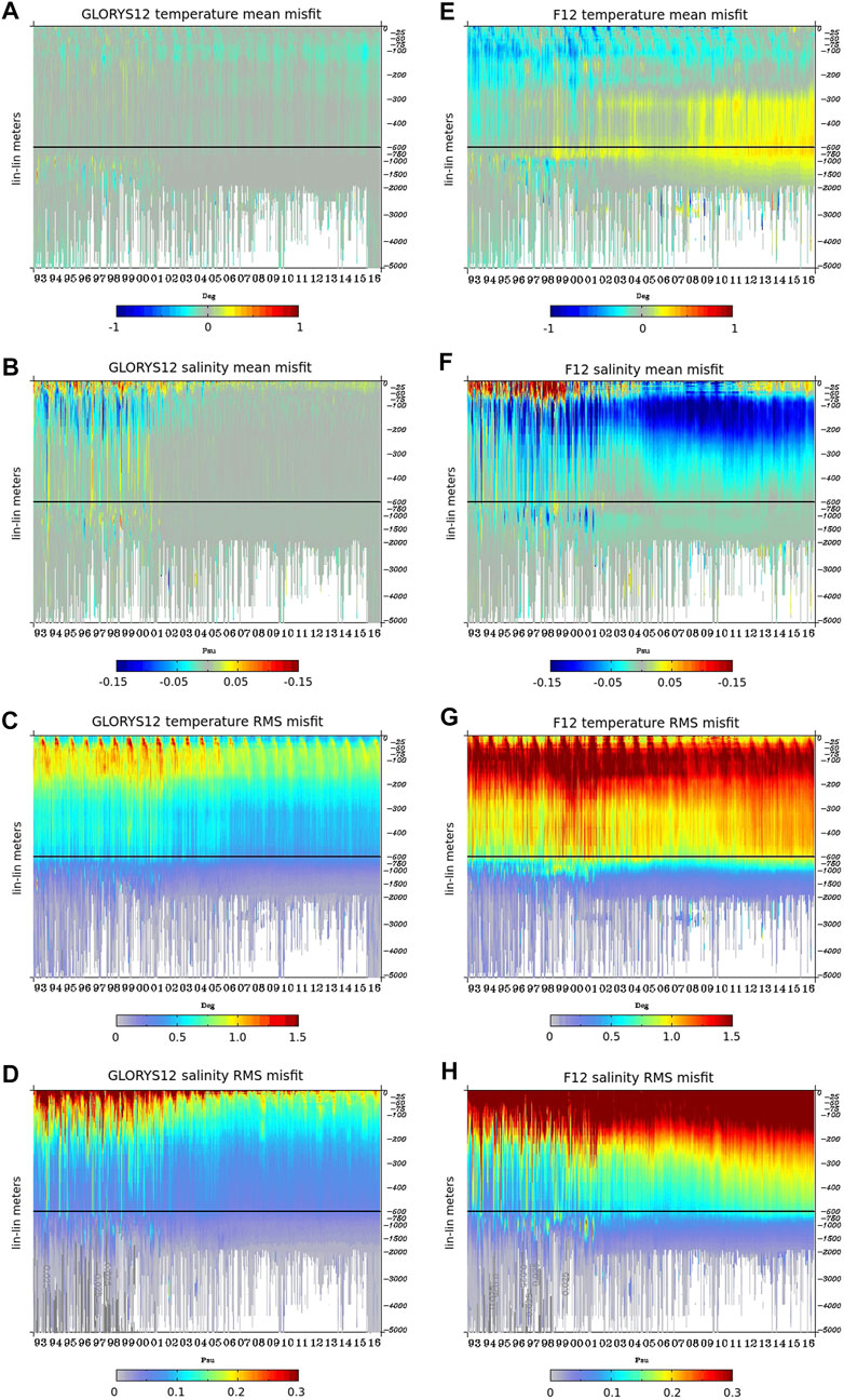
FIGURE 1. Assimilation diagnostics with respect to the vertical temperature and salinity profiles over the 1993–2016 period. Mean misfits (observation minus background model first trajectory) for temperature (A,E) and for salinity (B,F) and RMS misfits for temperature (C,G) and for salinity (D,H). Left panels (respectively right panels) concern GLORYS12 (respectively F12). These scores are averaged overall seven days of the data assimilation window, with a mean lead time equal to 3.5 days. Units are °C for temperature and psu for salinity.

From a more integrated point of view, Figure 2 shows the ability of the different systems GLORYS12, F12 and G4 in reproducing observed temperature and salinity in the 0–2,000 m layer. For that, we checked time series of the RMS difference between the model and the observations for temperature and salinity where observations are available in the water column. We compare also the observations to the Levitus WOA13 monthly temperature (Locarnini et al., 2013) and salinity (Zweng et al., 2013) climatology. We first note that the vertically integrated accuracy of GLORYS12 is very similar to that of G4, even if GLORYS12 slightly outperforms G4 throughout the 1993–2016 period. Between 1993 and 2002, departures from in situ observations are around 0.75°C for temperature and 0.2 psu for salinity. The average accuracy reaches 0.45°C in temperature and 0.1 psu in salinity during the Argo period, thanks to the increase of the number of observations assimilated in G4 and GLORYS12. For salinity, the statistics are very noisy before 2004 due to very sparse data that are not representative of the global state of the oceans. The departure between climatology and observations is an indicator of the minimum performance that the system must achieve. G4 and GLORYS12 temperatures are both significantly more accurate than the climatological temperature throughout the period. For salinity, the reanalysis clearly outperforms the climatology only after 2013, when the number of observations has doubled since the beginning of the Argo era. The free simulation F12 nearly always exhibits far lower scores than the climatology. The only exception takes place when F12 captures the very strong El Niño-Southern Oscillation (ENSO) signal in temperature in 1997/1998, and thus F12 is closer to in situ observations than the climatology can be during these two years, even on global average. The F12 RMS differences reach in 2016, 1°C for temperature and 0.2 psu for salinity, twice the RMS departures obtained with GLORYS12. Worse, we can observe a tendency for these errors to increase between 2008 and 2016, showing the drift of the system without data assimilation.

FIGURE 2

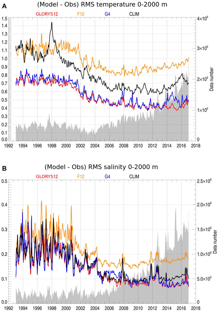
FIGURE 2. Time series over the 1993–2016 period of the 0–2,000 m RMS difference between the model analysis (best model trajectory) and the in situ T/S observations from the CORA database for GLORYS12 (in red), F12 (in orange), G4 (in blue) and Levitus WOA13 climatology (in black): (A) Temperature (units in °C), (B) salinity (units in psu). Time series of the number of available observations appear in grey.

Comparison With Satellite Sea Level Anomaly

The assimilation of sea level anomalies together with the MDT is crucial for the realism of the reanalysis’s ocean circulation. The statistics in Figure 3 use innovations and residuals coming from the sea level anomalies data assimilation. Residuals include the analysis correction injected into the model using incremental analysis update. The scores are averaged over all 7 days of the data assimilation window, which means the results are indicative of the average performance of GLORYS12 over the 7 days, with a mean lead time equal to 3.5 days.

FIGURE 3

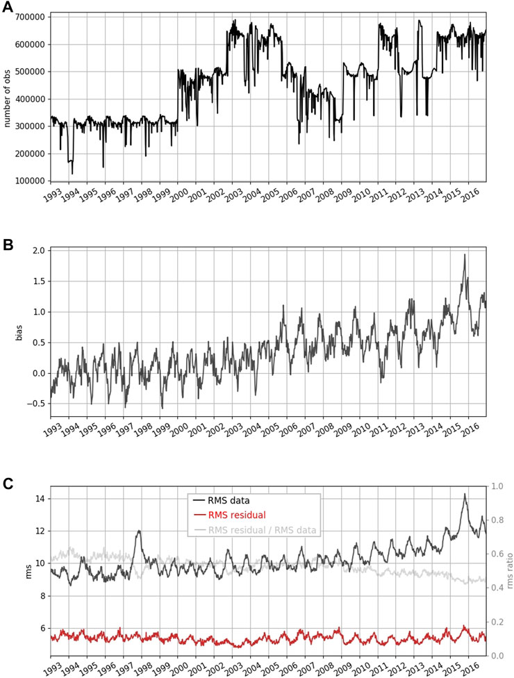
FIGURE 3. Time evolution of SLA data assimilation statistics averaged over the whole domain: (A) data number, (B) mean innovations, (C) RMS of the SLA data (in black), RMS of residuals (in red), RMS of residuals divided by RMS of SLA observations (in light grey, with the scale on the right). The scores are averaged over all seven days of the data assimilation window, with a lead time equal to 3.5 days. Units are cm.

The number of assimilated SLA observations (Figure 3A) varies with the number of altimeters in-flight throughout the period 1993–2016. This 24 year period involves eleven different altimeters. Following TOPEX-Poseidon in September 1992, the constellation has grown from one to six satellites flying simultaneously, even if we can notice a temporary decrease between 2005 and 2010.

The biases are weak in the 1990s, as the mean innovations vary around zero (Figure 3B). However, from 2004, a bias is diagnosed, which tends to increase and reaches 1 cm at the end of the period, with peaks varying from 1 cm or even 2 cm at times. This means that GLORYS12 tends to become too low in comparison with altimetry by about 0.25 mm per year. This bias is predominantly associated with the orbit standard used in the assimilated sea level anomalies (Taburet et al., 2019, their Figure 8B). Despite this bias, the reanalysis is close to altimetric observations with a residual RMS difference of the order of 5.5 cm on global average (Figure 3C, red curve). This RMS difference is consistent with the a priori prescribed observation error, which is equal to the sum (in variance) of the SLA instrumental error (about 2 cm on average) plus the MDT error (about 5 cm on average, with the largest values being located on shelves, along the coast and mesoscale activity or sharp front areas). This good performance is partly due to the use of the “Desroziers” method (Desroziers et al., 2005) to adapt the observation errors online, which yields more information from the observations being used (see Lellouche et al. (2018) for more details). Moreover, the model is able to explain the observed signal Figure 3C, black curve) as shown by the ratio of RMS residual to RMS data (Figure 3C, light grey curve), which decreases with time and converges towards a value much less than one. The performance of GLORYS12 remains stable and even improves while the variance of observations increases.

Comparison With Satellite Sea Ice Observations: Mean State and Low Frequency Variability

This section focuses on the ability of GLORYS12 to reproduce the mean state, expressed in terms of the mean seasonal cycle, interannual variability and trends over the 1993–2016 period, of spatially integrated quantities such as sea ice extent and volume and amount of open waters within the sea ice pack. The sea ice extent is usually defined as the area of ocean with a sea ice concentration of 15% or more. Sea ice area is the total area covered only by sea ice and is always less than the extent. The difference gives the amount of open water in the ice pack. The latter quantity then represents both the presence of leads within the sea ice pack and the marginal ice zone (MIZ) close to the ice edge. This quantity is collectively referred to as “leads” in the subsequent text.

To assess the overall consistency with observations we compare modelled sea ice extent and leads to the observational product CERSAT assimilated in GLORYS12, and to the mean of the ensemble of three observational products (CERSAT, NOAA/NSIDC, and OSI-SAF) which provides an estimate of the observational error. The NOAA/NSIDC passive microwave sea ice concentration climate data record (CDR) is an estimate of sea ice concentration that is produced by combining concentration estimates from two algorithms developed at the NASA Goddard Space Flight Center: the NASA Team algorithm (Cavalieri et al., 1997) and the Bootstrap algorithm (Comiso, 2000). The final CDR value is the highest between concentrations estimated by Bootstrap and NASA Team. OSI-SAF (Ocean Sea Ice Satellite Application Facilities), produced by EUMETSAT and distributed by CMEMS, is currently assimilated by the Arctic and in the PSY4V3 monitoring and forecasting systems of CMEMS. These two latter observational products are the datasets most widely used by the sea ice community. Other sea ice concentration algorithms exist and the subsample of products used in this paper is not sufficient to fully assess the uncertainty of the observations (e.g., Ivanova et al., 2015).

Arctic Ocean

In the Arctic Ocean, compared to the assimilated CERSAT data, GLORYS12 has a larger sea ice extent during winter time and a similar extent during summer time (Figure 4A). GLORYS12 sea ice extent largely remains in the spread of the observation based products, an ensemble in which CERSAT represents the member having the least sea ice extent. GLORYS12 constantly stays in the lower bound of the GREP product which shows a constant overestimation with a large spread during summer time. GLORYS12 favorably reduces the amplitude of the sea ice extent seasonal cycle simulated by F12. Similar conclusions are found with the sea ice concentration variable (not shown). The increase of resolution (GLORYS12 versus G4) has no visible impact on the mean state (seasonal cycle), the interannual variability and the trend of sea ice extent, leads and volume (Figure 4).

FIGURE 4

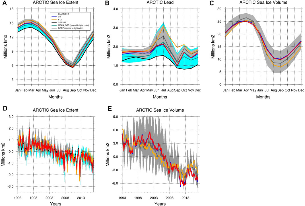
FIGURE 4. Arctic Ocean–Mean seasonal cycle (1993–2016) of (A) Sea ice extent, (B) Sea ice leads, and (C) Volume. Interannual monthly variability of (D) Sea ice extent and (E) Sea ice volume. Units are in million km² for sea ice extent and leads and in million km³ for sea ice volume. GLORYS12 (red), F12 (orange), G4 (blue), GREP (dark grey with the spread in light grey), mean observations (dark cyan with the spread in cyan) among CERSAT (black), NOAA/NSIDC (not shown) and OSI-SAF (not shown).

The presence of open waters within the GLORYS12 sea ice pack is much larger than in the assimilated CERSAT data (Figure 4B). This is particularly true during the melting season (June-August), period of the maximum of the surface covered by the MIZ, where GLORYS12 shows an excess of half a million km² during July. However, the large spread of the observation based products all along the year indicates large uncertainties in sea ice concentration algorithms retrievals. This is particularly true during summertime where this spread represents nearly the same amount of MIZ estimated by CERSAT. CERSAT data represents the lower bound of the large spread of the observations and GLORYS12 matches particularly well the ensemble mean of the observations. The spread shown around the GREP mean ensemble (Figure 4B) highlights how different physical parameterizations and/or assimilation methods within the four members of GREP can impact the representation of open waters within the Arctic sea ice pack.

F12 simulates a larger surface covered by leads and MIZ all through the year compared to GLORYS12. The assimilation of sea ice concentration therefore tends to reduce the presence of open water within the sea ice pack. The methodology for the mean analysis update of sea ice thickness adopted in GLORYS12 results in a general thicker sea ice cover compared to F12. Comparisons with in situ data in the Western Basin (Figure 5B) and in the Central Basin (Figure 5C) confirm a general thicker ice in GLORYS12. The unrealistic piling up of sea ice thickness in the Beaufort Gyre present in all GLORYS reanalysis (Chevallier et al., 2017; Uotila et al., 2019) is also present in GLORYS12. Comparisons with Cryosat-2 in January 2014 (Figure 5A) show an overestimation of the order of almost 1 m in the area. This overestimation is confirmed by comparisons with in situ data from the BGEP campaign (Figure 5B). This ice build-up prevents efficient melting and ends up with generally thicker sea ice conditions in summertime. This phenomenon occurs as soon as the assimilation of sea ice concentration data is activated, e.g. during summer 1993. Comparisons with Cryosat-2 also show that this unrealistic ice accretion in the Western Basin is accompanied, however, by thinner sea ice conditions in Central and Eurasian basins (Figure 5A). Comparisons with in situ data from the NPEO campaign confirm the presence of thinner ice in GLORYS12 in the Central Arctic Basin (Figure 5C). Nevertheless, GLORYS12 improves the too thin sea ice cover found in F12 in the Central Arctic Basin, e.g. in areas of multi-year ice types. The resulting total sea ice volume is improved compared to the previous Mercator Ocean reanalysis system G2V4 (Chevallier et al., 2017; Uotila et al., 2019) and compares better with PIOMAS data (Schweiger et al., 2011). Over the same period (1993–2016), the seasonal cycles of GLORYS12, F12, G2V4 and PIOMAS have respective minimums and maximums of 9.8 and 25 million km³, 6.9 and 25.5 million km³, 13.2 and 28.3 million km³, and 9.4 and 25.7 million km³.

FIGURE 5

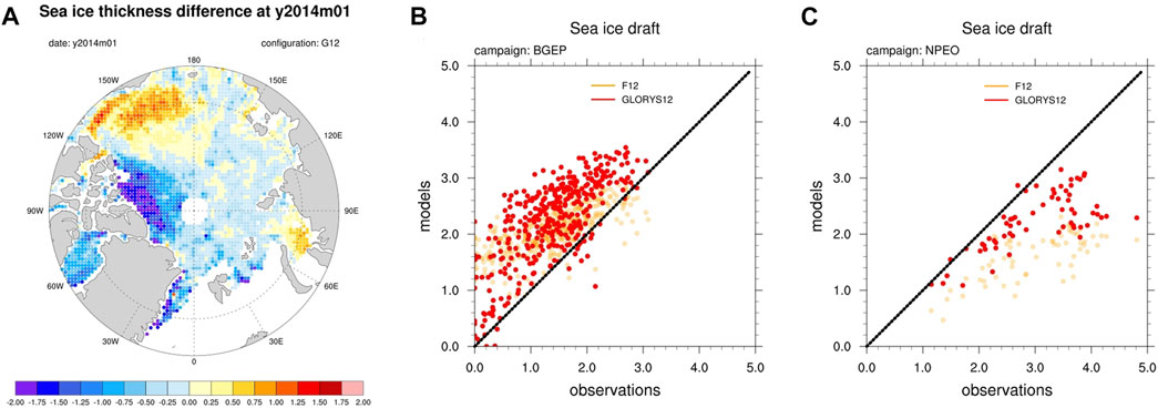
FIGURE 5. (A) Differences of sea ice thickness between GLORYS12 and Cryosat-2 data (Ricker et al., 2014). Model versus observations plots of sea ice drafts on a linear scale with GLORYS12 (red) and F12 (orange) and in situ observations from (B) BGEP (Beaufort Gyre Exploration Project, (Krishfield et al., 2014)) campaign, (C) NPEO (North Pole Environment Observatory, (Drucker et al., 2003)) campaign.

The large spread in the sea ice volume present in the GREP multi-model product again reflects the impact of the disparity in assimilation methods and parameterizations applied in these reanalyses (Figure 4C).

CERSAT data show a significant (95%-level confidence) and negative trend in sea ice extent at a rate of −79 900 km²/yr and observation based products at a rate of −77 300 km²/yr. The simulation without assimilation F12 already reproduces this negative linear trend with a somewhat overstated rate of −86 850 km²/yr. Both reanalyses (GLORYS12 and G4) with respectively −85 320 and −84 000 km²/yr trends, favorably reduce this strong loss of surface covered by sea ice in the Arctic Ocean. With −89 400 km²/yr, the GREP ensemble mean has a stronger trend compared to GLORYS12. The spread among GREP members narrowed somewhat after 2010, a period marked by a succession of historic summer lows. These latter results are similar to those presented in the GREP-based Ocean Monitoring Indicators (OMI) sea ice extent (https://marine.copernicus.eu/access-data/ocean-monitoring-indicators/northern-hemisphere-sea-ice-extent-multi-model-ensembles). The weak interannual trends of the surface covered by leads and MIZ found either with the reanalysis or with the observations are not significant and are therefore not discussed.

The most important differences between GLORYS12 and F12 are in the reproduction of interannual variability and trend in sea ice volume. The strong accumulation of ice that became thick in the late 1990s and early 2000s shown in GLORYS12 is not in F12 (Figure 4E). The resulting trend is consecutively more pronounced in GLORYS12 than in F12, respectively −465 900 and −380 800 km³/yr. These trends can be compared with that of PIOMAS from about −427 100 km³/yr over the same period (1993–2016). Once again, the spread present in GREP product at this lower frequency variability highlights the large uncertainty in the representation of Arctic sea ice volume by the different reanalysis products (Chevallier et al., 2017).

Antarctica

As for the Arctic Ocean, GLORYS12 and G4 reanalyses have very similar results in Antarctica. F12 faces a consistent bias found in many models (Roach et al., 2018) and simulates a sea ice cover with too low sea ice concentrations throughout the year (not shown). As a result, and under unknown triggering effects, a first window through the sea ice occurred in winter of 1997 in eastern part of the Weddell Sea and started to transfer energy during winter between the ocean and the atmosphere. This energy exchange broke the stratification present at the surface, e.g. warm and salty waters overlaid by fresh surface waters, and started to homogenize the water column by vertical motions. The unusual presence of these relatively warmer waters on the surface prevented the formation and presence of ice locally. This phenomenon has persisted from one year to the next and spread to wider areas. The ice cover could never return to its normal extent, especially in winter (Figure 6A). Thanks to the assimilation of sea ice concentration, GLORYS12 avoids this behavior and keeps a seasonal cycle very comparable to observations (Figure 6A). GLORYS12 exhibits a sea ice extent very close to the observations with, however, and as in the Arctic, a tendency to have a slightly higher extent, particularly in winter. Further, GLORYS12 sea ice extent is within the spread of the GREP ensemble.

FIGURE 6

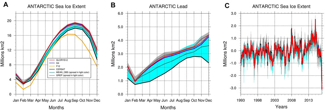
FIGURE 6. Antarctica - Same as Figure 4 for mean seasonal cycle (1993–2016) of (A) Sea ice extent, (B) Leads, and (C) interannual monthly variability of sea ice extent. The simulation F12 is not shown in panels (B,C).

As in the Arctic, the CERSAT data (extent and leads), are the lowest estimates of all observations. The lead observations spread is much larger than that of GREP and even reaches 2 million km² in the spring, the equivalent of the total lead area estimated by CERSAT. GLORYS12 sea ice extent and surface of leads are within the spread of the GREP ensemble. The Antarctic sea ice extent in spring 2016 attained a record minimum (Turner et al., 2017) for the 1993–2016 period, presenting an abrupt departure from the slowly but steadily expanding until several monthly record high in 2014. Combined with this high variability, the resulting weak positive trend found in all reanalyses and all observations is not significant (95%-level confidence). This non-significance is in agreement with the study of Yuan et al. (2017).

Large-Scale Dynamics

Meridional Heat Transport and Inter-Basin Volume Exchanges Transports

Large-scale ocean transports play a major role in the Earth Climate. Various estimates of global heat and mass transports at key sections have already been calculated from direct ocean hydrographic sections (Talley et al., 2003), from the World Ocean Circulation Experiment based on the inversion of hydrographic data (e.g., Ganachaud and Wunsch, 2003; Lumpkin and Speer, 2007), and from ocean reanalyses (e.g., Stammer et al., 2004; Haines et al., 2012; Valdivieso et al., 2017). More recently, Bricaud et al. (2018) gave estimations of volume transports through key sections from GREP and of meridional heat transport (MHT) based on the 1/4° reanalysis G2V4 and its associated free run for the three major basins (global, Atlantic and Pacific+Indian). In this section, we provide estimations of GLORYS12, G4 and F12 MHT and volume transports through key sections and compare them to observation-based estimates and to GREP product.

Given large uncertainties linked with the oceanic observations sampling, Figure 7 shows a good agreement of transport estimates between volume transports through different sections from GREP product and from Lumpkin and Speer (2007) (Figure 7A) with a median value of the relative error of 30%, and the same diagnostics for GLORYS12, F12 and G4 (Figure 7B).

FIGURE 7

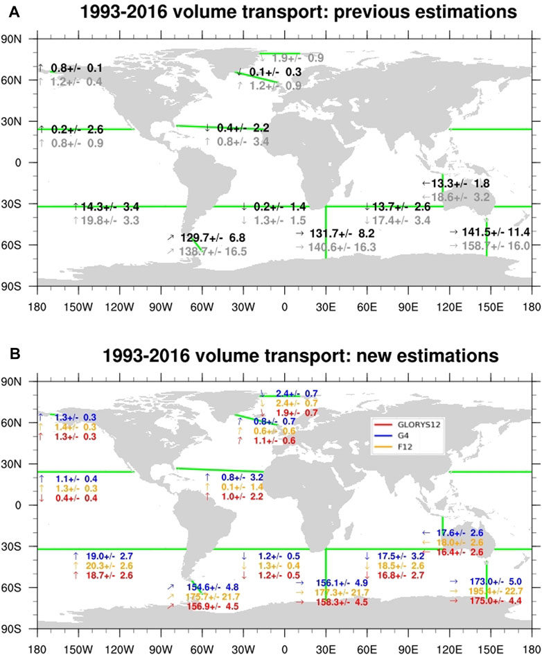
FIGURE 7. Mean volume transport and its variability for the 1993–2016 period from (A) Lumpkin (in black) and GREP 1/4° ensemble product (in grey) and from (B) GLORYS12 (in red), F12 (in orange) and G4 (in blue). Units are in Sv.

GLORYS12 reanalysis transport at Drake Passage has been particularly and extensively studied in Artana et al. (2019b). The authors show that GLORYS12 estimates are within recent observation-based estimates (8 Sv larger than Koenig et al. (2014) estimate and well below the estimate of 173.3 ± 10.7 Sv using measurements from the cDrake project (Donohue et al., 2016)) and especially emphasizes that accurately assessing the absolute transport through Drake Passage remains a challenge. However, with respectively 156.9 ± 4.5 and 154.6 ± 4.8 Sv, GLORYS12 and G4 transports at Drake Passage are very close to each other and considerably reduce the transport estimate compared with that from the simulation without assimilation F12. Artana et al. (2019b) have shown that the mean volume transport of GLORYS12 over 1993–2010 (157 ± 3 Sv) is similar to a nine-ensemble mean of 152 ± 19 Sv over the same period from lower resolution global reanalyses (resolution ranging from 1° to 1/4°, five are of European origin using varying versions of the NEMO ocean, three are American and one is Japanese) (Uotila et al., 2019). Antarctic Circumpolar Current (ACC) transports in both GLORYS12 and G4 are in the spread of the GREP NEMO-based ensemble but remain in the upper bound of this set of estimates. It is also larger than Lumpkin’s estimates.

Compared to the canonical climatological estimation of 0.8 Sv from Woodgate et al. (2006), the Bering Strait transport is larger in both GLORYS12 and G4 (1.3 Sv). Both GLORYS12 and G4 estimates are closer to the most recent estimates, which show that, over the last decade, volume transport in Bering Strait has been steadily increasing and is now well above 1 Sv (Woodgate,2018). Both GLORYS12 and G4 estimates (1.3 Sv) favorably reduce the too strong F12 transport (1.43 Sv).

As the only deep water passage to the Arctic Ocean, transports through Fram Strait determine to a large extent the exchanges between the North Atlantic and the Arctic Ocean. With respectively, 1.9 ± 0.7, 2.4 ± 0.7, and 2.4 ± 0.7 Sv, GLORYS12, G4 and F12 are close to the canonical observation-based estimates of ∼2 Sv from Fahrbach et al. (2001). At Fram Strait and at the Greenland-Iceland-Scotland section, GLORYS12 transports are identical to GREP estimations.

Generally, GLORYS12, G4 and all reanalyses included in GREP provide transport estimates that are higher than values deduced from observations, whether at high latitudes, as just mentioned, or at tropical latitudes (Indonesian Throughflow and meridian sections at 30°N and 30°S, Figure 7A).

Meridional heat transports for the three major basins (Figure 8) are estimated using 5 day mean fields in order to avoid aliasing errors found with monthly mean sampling (Crosnier et al., 2001). MHTs in GLORYS12 and G4 are in general very close to each other. In Global and Pacific-Indian basins, GLORYS12 and G4 differ at the Equator where a strong gradient is present in their respective MHT. For the Global basin, the MHT peak at 5°N is 1.2 PW for GLORYS12 and 1.6 PW for G4. For the Pacific-Indian basin, the MHT peak at 5°N is 0.2 PW for GLORYS12 and 0.7 PW in G4. In the Atlantic basin, they differ at 40°N, where MHT is 1.2 PW for GLORYS12 and 1.4 PW in G4. Compared to G4, GLORYS12 then simulates higher MHT northward poleward transport in regions with strong gradients (equatorial dynamics and Gulf Stream current). Conversely, GLORYS12 displays lower values in the [40°S–60°S] latitude band of the Antarctic Circumpolar Current (ACC) fronts compared to G4 estimates.

FIGURE 8

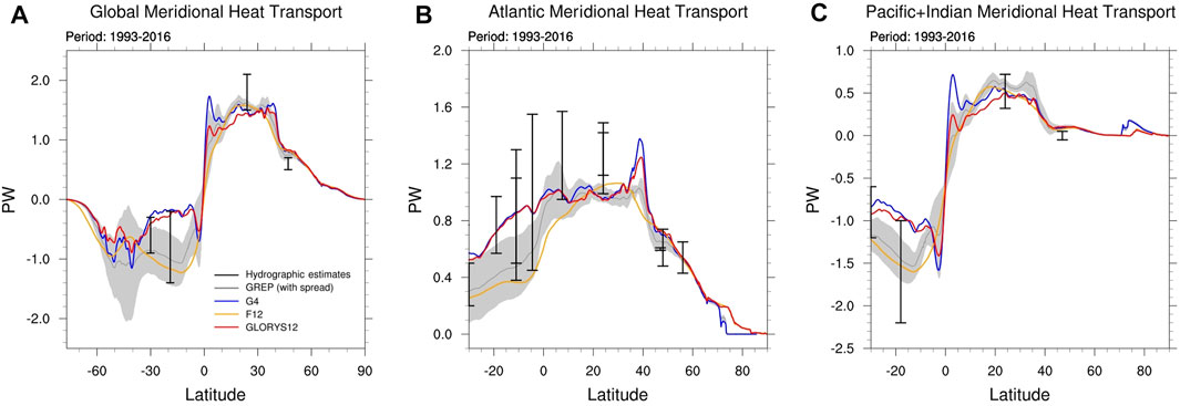
FIGURE 8. Mean Meridional Heat Transport for the 1993–2016 period for Global Ocean (A), Atlantic Ocean (B) and Pacific + Indian Oceans (C). GLORYS12 is plotted in red, F12 in orange, G4 in blue, GREP ensemble product in grey and hydrographic estimates in black. Units are PW.

GLORYS12 and G4 MHTs greatly differ from F12 in the Southern subtropical gyres with a significant stronger northward heat transport in the [40°S–20°N] latitude band. This results in a weaker poleward heat transport by Southern tropical gyres in reanalyses than in the simulation without assimilation. While this weakening is more consistent with the error bars in the Atlantic, it drives heat transport out of the error bars in the Indo-Pacific. However, the error bars proposed by Ganachaud and Wunsch (2003) or Lumpkin and Speer (2007) are very large, particularly in the tropical band of the Atlantic Basin.

In GLORYS12 and G4, the Global and the Pacific-Indian basins equatorial MHT gradient is stronger than in F12. The current interpretation is that those peaks are overestimated due to spurious velocities induced in particular by the assimilation of SLA (and MDT) in the equatorial region (Gasparin et al., 2021). For the Global basin, F12 MHT is lower than GLORYS12 and G4 MHTs in the [40°S–0°] latitude band and close to lower values of the hydrographic estimates, whereas GLORYS12 and G4 MHTs are close to the upper values of the hydrographic estimates. For the Atlantic basin, F12 MHT is lower than GLORYS12 and G4 MHTs in the [30°S–20°N] latitude band and close to lower values of the hydrographic estimates, whereas GLORYS12 and G4 MHTs are close to the middle values of the hydrographic estimates. For the Pacific-Indian basin, F12 MHT is lower than GLORYS12 and G4 MHT in the [30°S–0°] latitude band and close to middle values of the hydrographic estimates, whereas GLORYS12 and G4 MHTs are close to the upper values of the hydrographic estimates.

Moreover, the time mean state and interannual-decadal variability of the North Atlantic ocean since 1993 have been assessed in Jackson et al. (2019). The authors show that GLORYS12 is able to reproduce the main aspects of the circulation including convection, AMOC and gyre strengths, and transports.

Velocity Validation Against Drifter’s Estimation

In this section, we use velocity observations from surface drifters (that are not assimilated) to assess the level of performance of GLORYS12 qualitatively. To avoid contamination by the windage due to a drogue loss (Grodsky et al., 2011), we use the drogued-only 15 m drifter dataset coming from the CMEMS in situ Thematic Assembly Centre (Rio and Etienne, 2019). Model counterparts of the drifter’s velocities are interpolated at the right time and averaged over the 2003–2016 period. Results at 15 m (Figures 9A,B) are very similar to those from the CMEMS real time system (Lellouche et al., 2018). The general circulation with major currents is well represented. The main shortcoming concerns the tropical Pacific South Equatorial Current which is too strong in GLORYS12. It has been shown that this was mainly due to a bias in the reference height for the altimetry (Hamon et al., 2019). It can also be noted that the ACC is slightly too strong near the surface. We now use estimated velocities at 900 m derived from Argo profiling floats when drifting at their parking depth (Lebedev et al., 2007). Comparisons in panels C and D of Figure 9 show a good general agreement between the observations and GLORYS12. The ACC has the right intensity at this depth. This is consistent with Thoppil et al. (2011) results which show that high-resolution model and data assimilation improve the representation of fine structures at depth at high latitude. The only notable differences concern the striations of the equatorial band (Cravatte et al., 2017) which are slightly underestimated and not reproduced at the right latitude by GLORYS12.

FIGURE 9

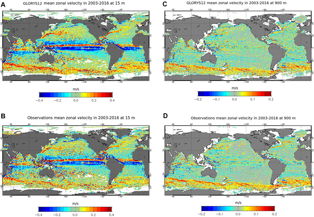
FIGURE 9. Panels (A,B): mean zonal velocity at 15 m over the 2003–2016 period for GLORYS12 (A) and observations (B). Observations come from drogued-only subsurface drifters (Rio and Etienne, 2019). Panels (C,D): mean zonal velocity at 900 m over the 2003–2016 period for GLORYS12 (C) and observations (D). Observations come from estimated velocities derived from Argo profiling floats (Lebedev et al., 2007). Units are m/s.

Ocean Variability

Eddy Kinetic Energy

In order to estimate the mesoscale activity present in GLORYS12, comparisons of geostrophic Eddy Kinetic Energy (EKE) deduced from GLORYS12 and from F12, G4 and the L4 CMEMS DUACS gridded product (Taburet et al., 2019) have been performed over the 2007–2016 period. These comparisons are made over the last 10 years of the 1993–2016 period to ensure that the simulations, in particular F12, have reached a state of equilibrium (see Eddy Kinetic Energy Time Evolution). Geostrophic EKEs of GLORYS12, F12, and G4 are deduced from daily sea surface height (SSH) from which geostrophic velocities are computed. Geostrophic EKE of the DUACS product is calculated directly from the daily geostrophic velocities included in the product.

Figure 10 shows the geostrophic EKE for GLORYS12 (panel A), and the differences against the three others estimates: GLORYS12 minus DUACS (panel B), GLORYS12 minus F12 (panel C) and GLORYS12 minus G4 (panel D). We observe very realistic structures in GLORYS12. All the large dynamic systems are very well represented (Western Boundary Currents (WBCs), Agulhas recirculation, Leeuwin Current, ACC). Compared to DUACS, the differences in the major currents are small. However, we observe a higher level of EKE almost everywhere of 25–50 cm²/s². DUACS shows stronger EKE levels at some specific locations, such as the equatorial band (10°S–10°N) and towards Madagascar. These departures from DUACS are consistent with that depicted by Chassignet and Xu (2017) for models at 1/25° and 1/50° resolution without data assimilation. The authors show that using proper temporal and spatial filtering, similar energy levels can be found between different databases. Still, the direct comparison with the EKE derived from the DUACS maps remains complex because DUACS maps do not include the smaller space and time scales that are filtered out through the mapping procedure. In particular, DUACS underestimates the EKE by more than 20% in the mid and high latitudes (Le Traon and Dibarboure, 2002).

FIGURE 10

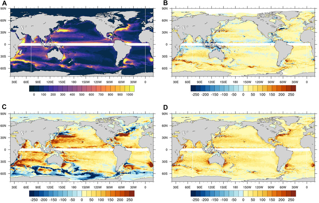
FIGURE 10. Geostrophic Eddy Kinetic Energy over the 2007–2016 period for GLORYS12 (A) and differences against the three others estimates: GLORYS12 minus DUACS product (B), GLORYS12 minus F12 (C) and GLORYS12 minus G4 (D). Units are cm²/s².

Comparing GLORYS12 to F12, one can observe strong differences, especially in the WBCs where the incorrect positioning of the currents in the free simulation creates large dipoles on the difference map. These differences show that data assimilation helps positioning better the main observed currents in GLORYS12. Almost everywhere, except the ACC, the energy level in GLORYS12 is significantly higher than the energy level in F12, with differences varying from 50 to 150 cm²/s². This means data assimilation potentially adds information everywhere in the model dynamics, with a strong signature in EKE. It is important to mention that the EKE level in F12 is of the same order of magnitude than that of other simulations with equivalent resolution and without data assimilation, as presented in Chassignet et al. (2020) (not shown). The increase of EKE in GLORYS12 does not correct a potential underestimation of the energy level by F12. GLORYS12 can add new information such as the breakdown of internal waves, but can also limit the attenuation of mesoscale activity in F12 via the assimilation of the SLA. Nevertheless, in the ACC, F12 is more energetic than GLORYS12. The reason of this difference is still not explained and requires further investigations. The comparison between GLORYS12 and G4 shows a general increase in the EKE level with increasing resolution. This overall increase is approximately 10%. The stronger EKE in GLORYS12 is an expected direct effect of the increase of resolution, allowing the representation of small structures.

Quantification of Energy Gain

To go further in the understanding of the energy level in GLORYS12, a spectral analysis is performed in order to quantify the energy gain in GLORYS12 SST analyses (with respect to G4 and F12) at different spatial scales. A local spectral decomposition was made on SST from daily model outputs during the year 2013, which is a neutral year considering the North Atlantic Oscillation and ENSO indices. Moreover, working over a single year has the advantage of avoiding mixing structures placed differently according to climatic indices.

For each point of a regular subsampling of the GLORYS12 model grid (one point in ten), a mean power spectral density (PSD) is obtained by averaging the results over the four main directions S-N, W-E, SW-NE, and NW-SE. In practice, the decomposition is performed using the one-dimensional SST signal over the four 1,000 km synthetic continuous tracks centered on the regular subsampled grid points. In order to avoid sampling issues, G4 outputs have been first interpolated on the same grid as GLORYS12. This methodology is directly derived from that of Dufau et al. (2016), used for spectra calculation along altimetry tracks. As expected, the overall average results confirm that GLORYS12 contains more energy at finer scales (not shown). We also find that G4, F12, and GLORYS12 have roughly the same energy at large scales but the difference between GLORYS12 and the two other configurations tends to increase towards the smaller scales. The difference between GLORYS12 and G4 are less than 20% around 200 km. The difference between GLORYS12 and F12 is about 20% near 55 km.

Focusing on the typical length scale of the mesoscale activity (50–250 km range), Figure 11 shows that the power gain is evenly distributed over the entire ocean. Panels (A–C) show the local percentage of power in the mesoscale band normalized by the total power (in the 20–980 km band) for G4, GLORYS12 and F12 respectively. The comparison between the maps highlights the local change in the slope of the PSD (not shown). Except for the equatorial area, constrained mainly by large-scale atmospheric phenomena, it appears that the SST in GLORYS12 is the most energetic in the mesoscale part of the spectrum. Given the logarithmic behavior of the energy spectrum, the average difference of one percent between the power fraction of the mesoscale energy of GLORYS12 and G4 remains significant. The data assimilation has also a small effect on the mesoscale power fraction. Thus, GLORYS12 is uniformly more energetic than F12 in the global ocean, except the Northern part of the Atlantic.

FIGURE 11

FIGURE 11. Power fraction in the mesoscale (50–250 km) band normalized by the total power in the 20–980 km band for G4 (A), GLORYS12 (B) and F12 (C) SST in year 2013. Units are %.

Eddy Kinetic Energy Time Evolution

Three-dimensional average EKEs can also be assessed from GLORYS12, F12, and G4 daily velocity fields. Figure 12A shows the temporal evolution of the three-dimensional mean of monthly EKEs deduced from velocity. No observation comparison is available since a three-dimensional total EKE cannot be deduced from the observations. Consistently with the surface geostrophic component (Figure 10), GLORYS12 is more energetic compared to G4 and F12. The average value is equal to 14 cm²/s² for GLORYS12, 10 cm²/s² for F12 and 8.5 cm²/s² for G4. Simulations start from rest and a first stabilization of the energy level occurs after 1 year for the simulations with data assimilation (GLORYS12 and G4) and after 3 years for F12, corresponding to the spin up time needed for model simulations to reach their energetic equilibrium. The seasonal cycle is well marked in all time series and after the first three years, important interannual variations are present, as in 1997–1998 with the strong ENSO event which induced a strong decrease of the global EKE.

FIGURE 12

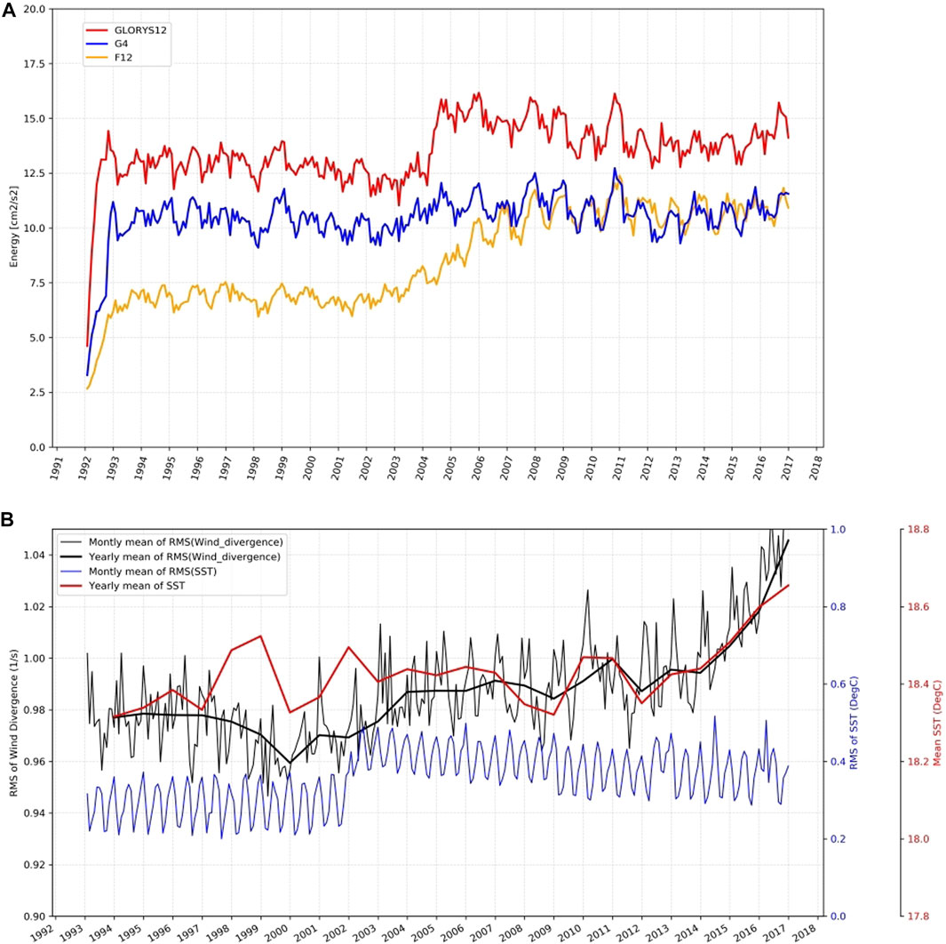
FIGURE 12. (A) Three-dimensional mean of monthly Eddy Kinetic Energy (in cm²/s²) for GLORYS12 (in red), F12 (in orange), G4 (in blue). (B) Monthly mean of spatial variance of daily SST (in blue), monthly (thin black) and yearly (thick black) mean of spatial variance of daily wind divergence, and yearly mean of SST (in red).

However, time series exhibit two main discontinuities. The first one occurs in the three simulations at the beginning of 2002 with an increase of energy until 2007. The strongest signature is observable in F12 with a change of mean state from 7 to 10 cm²/s². From 2002, an increase in the amplitude of the seasonal cycle is also observed in all simulations, where the intra-annual amplitudes change from 1 to 2 cm²/s². As this change of the system mean state is observed in the simulation F12 without data assimilation, it can therefore only come from atmospheric forcing. A deeper study of ERAinterim is needed to understand the behavior of GLORYS12, F12, and G4. ERAinterim is an atmospheric reanalysis derived from an atmospheric general circulation model with data assimilation but having boundary conditions at the interfaces of the atmosphere. In particular, ERAinterim uses a SST estimated from observations. The spatial resolution of SST products used during the production of ERAinterim changed from 1° to 0.5° (Dee et al., 2011) and this change induces modification of atmospheric circulation (Parfitt et al., 2017). Figure 12B (blue curve) shows the evolution of the spatial RMS of SST (a monthly mean has been applied to the daily data). The change of SST resolution in January 2002 is well marked with the increase reflecting the increase in variability. This change in the boundary condition of the reanalysis induces a change in the atmospheric fields and a modification of the wind field. Different mechanisms for adjustments of atmosphere to the oceanic small scales are described in many studies (e.g., Lindzen and Nigam, 1987; Hayes et al., 1989; Chelton et al., 2001; Spall, 2007; Minobe et al., 2008; Small et al., 2008; Renault et al., 2017). These local circulations do not appear on large-scale wind fields. It is therefore necessary to consider local circulations. These latter can be obtained by different filtering methods, but energy scales will depend on the filtering. If the divergence or rotational wind is considered, the smallest spatial variations of wind will be highlighted. The black curve in Figure 12B shows the spatial variability of the ERAinterim wind divergence. In 2002, the variations of wind divergence exhibit an increase at the same time of RMS SST variation. This demonstrates the atmospheric response to the SST change. After 2014 there is a strong increase which seems related to the increase in global average SST (Figure 12B, red curve). The increase in SST leads to more instabilities of the atmospheric column and therefore more divergence. However, this does not entirely translate into the energy transmitted to the ocean model. In summary, the increase in SST resolution in January 2002 results in an increase in small-scale variability in the atmospheric reanalysis winds, and part of this wind variability increase is transmitted to GLORYS12, F12, and G4. The second discontinuity occurs in 2004 where a strong and rapid increase is present in GLORYS12 (2.5 cm²/s² in 6 months) and one to a lesser extent in G4 (1 cm²/s²). No sudden increase at this date is observed in F12. This suggests that the source comes from data assimilation. In order to take into account the increase of the number of assimilated in situ T/S vertical profiles from January 2004 (see Figure 2), the time window in which the 3D-VAR bias correction is performed was reduced from 3 to 1 month in both G4 and GLORYS12. It would therefore seem that this reduction in the time window, combined with the increase in the number of assimilated in situ observations, creates an increase in energy and therefore changes the regime state of the system. This increase in energy is much more pronounced in GLORYS12 than in G4, due to the ability of GLORYS12 to create realistic mesoscale features.

Trends and Evolutions of Temperature, Salinity and Sea Level

Time Evolution of Temperature and Salinity Anomalies

Figure 13 shows the time evolution of temperature and salinity anomalies over the whole domain for F12, GLORYS12, and G4. An anomaly for a specific date is defined as the difference between the value at this current date and the initial state of the simulation. Note that for this diagnostic, the interannual signal has been removed using a digital time filter. GLORYS12 and G4 reanalyses show a warming in the 0–1,000 m layer (Figures 13C,E). It is a little too strong according to the mean misfits shown on Figure 1A. The freshening in the first 1,500 m (which occurs notably in the ACC) before Argo is present in G4 and to a lesser extent in GLORYS12 (Figures 13D,F). From the beginning of the year 2004, this freshening is strongly reduced in G4 and turns into a saltening in the first 200 m. This can be linked to the change in the time window to compute the T/S bias correction and by the increase in the number of assimilated profiles. Before the arrival of Argo floats in large quantity at the start of 2004, G4 and to a lesser extent GLORYS12 did not seem able to correct the salinity bias that had set in. GLORYS12 has a better behavior in salinity because the fronts are much better resolved in GLORYS12 than in G4, in particular the polar front which is poorly positioned in G4 (not shown). January 2002 seems to be a crucial date for F12 which presents a strong cooling in temperature in the 200–1,000 m layer, spreading at depth afterwards (Figure 13A). This behavior can be correlated to the change in the atmospheric fields discussed in Eddy Kinetic Energy Time Evolution. Moreover, the F12 simulation without data assimilation shows a strong salinity drift in the first 500 m (Figure 13B).

FIGURE 13

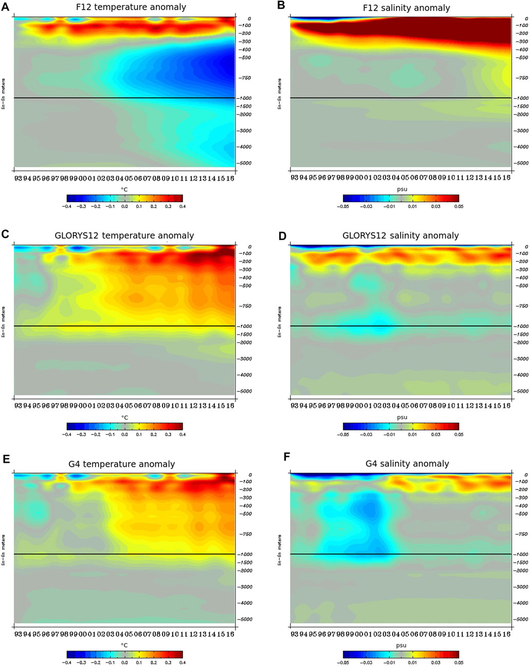
FIGURE 13. Time evolution of temperature (in °C, left panels) and salinity (in psu, right panels) anomalies over the whole domain for F12 (top panels A,B), for GLORYS12 (middle panels C,D) and for G4 (low panels E,F). An Anomaly for a specific date is defined as the difference between the value at this current date and the value at the initial state. The interannual signal has been removed using a digital time filter.

Sea Level Time Evolution

Of particular importance for sea level trends, along-track altimetric observations from various missions are assimilated in GLORYS12 and G4, together with in situ temperature and salinity profiles and other observations. Altimetric observations capture sea level trends due to land ice mass loss and land water storage changes, in addition to trends due to sterodynamic sea level changes (e.g., Gregory et al., 2019). As mentioned in the description of the ocean model in Description of GLORYS12, a global mean sea level (GMSL) trend is added at each time step to the modeled dynamic sea level. This added GMSL signal is composed of the diagnosed global mean steric sea level change and of a barystatic (land ice related, Gregory et al., 2019) sea level trend of 1.31 mm/yr over 1993–2001 and of 2.20 mm/yr over 2002–2016. The GMSL change is added to all simulations, prior to data assimilation for GLORYS12 and G4. In assimilated altimetric sea level observations, no correction has been applied for the drift of T/P-A over 1993–1998 (e.g., Beckley et al., 2017; Legeais et al., 2019), but regional GIA-related trends have been subtracted from the altimetric observations before assimilation (based on Peltier, 2004).

In terms of GMSL rise, G4 and GLORYS12 are in close agreement with altimetry (Figure 14). Yet, after 2004, G4 tends to better represent the seasonal cycle of GMSL changes than GLORYS12. The GMSL rise trend is also in closer agreement with altimetric observation (3.00 mm/yr over 1993–2016) in G4 (2.90 mm/yr) than in GLORYS12 (2.77 mm/yr). Although the barystatic sea level trend is added to the modelled sea level in all simulations (see Description of GLORYS12), the correct partition between the steric and barystatic components of GMSL changes is not yet ensured in GLORYS12 and G4. According to Figure 1A, there is an excess of heat storage around 100 m. As a result, the barystatic sea level trend is not fully retained in the system. Assimilation of altimetric sea level therefore leads to a too large global mean steric sea level rise in both G4 and GLORYS12. In GLORYS12, the global mean thermosteric sea level trend over 2005–2016 is 2.43 mm/yr (averaged over areas sampled by altimetry, Figure 15A). Thus, thermal expansion explains 70% of the GMSL trend of 3.20 mm/yr over the same period in GLORYS12, while it should only account for around 40% of the GMSL trend (Oppenheimer et al., 2019). As a result, the actual barystatic sea level trend in GLORYS12 over 2005–2016 is 0.77 mm/yr, instead of the 2.20 mm/yr added to the modelled sea level over 2002–2016. The issue in the separation of the barystatic and steric components of GMSL can be illustrated with the drop of around 5 mm in the altimetry derived GMSL in 2011 (Figure 14). This observed drop in GMSL is related to the 2010/11 El Niño event that led to more precipitation over Australia, northern South America and Southeast Asia. The corresponding ocean to land mass transfer increased the land water storage and accordingly decreased GMSL for months as the corresponding water was retained in endorheic basins (e.g., Boening et al., 2012). GLORYS12 and G4 also show a drop in GMSL in 2011. As only a barystatic sea level trend was added to GLORYS12 and G4, assimilation of altimetric data translated this mass signal into a steric signal, with an overall ocean cooling and contraction.

FIGURE 14

FIGURE 14. Global mean sea level monthly time series for the CMEMS gridded reprocessed altimetric dataset (007_048, in black), GLORYS12 (in red), F12 (in orange) and G4 (in blue). The global mean steric sea level of GLORYS12 is also shown (dashed red line). The same ocean mask has been used when computing the global mean. Only points with valid monthly means in altimetric sea level data along the whole 1993–2016 period have been used in the global mean.

FIGURE 15

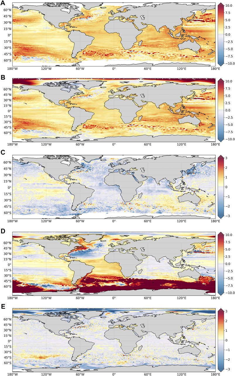
FIGURE 15. Regional sea level trends over the 1993–2016 period (in mm/yr) for (A) the CMEMS gridded reprocessed altimetric dataset (007_048), (B) GLORYS12, (C) GLORYS12 minus altimetric dataset, (D) GLORYS12 minus F12, (E) GLORYS12 minus G4. The global mean sea level trend has not been removed. No GIA correction has been applied to altimetric trends in panel (A). Note the different ranges covered by the color bars in panels (C,E).

Finally, the free simulation F12, where no GMSL correction is applied, exhibits a very low GMSL rise (0.75 mm/yr over 1993–2016, Figure 14), highlighting the benefits from data assimilation to represent GMSL changes. The steric part of GMSL rise in F12 is close to zero in the 1990s and then drops to negative values (cooling (see Time Evolution of Temperature and Salinity Anomalies and Figure 13A), especially in the Southern Ocean (not shown)), explaining the low GMSL trend in F12.

At regional scales, sea level trends over the 1993–2016 period in GLORYS12 are in close agreement with sea level trends inferred from the CMEMS reprocessed and gridded altimetry product (Figures 15A,B). The main patterns of sea level trends observed by altimetry (e.g., Forget and Ponte, 2015; Dangendorf et al., 2019) are captured in the reanalysis, with the largest trends in the western tropical Pacific, northwestern Pacific, northern Southern Ocean, and the lowest trends in the subpolar North Atlantic, off Alaska, in the eastern tropical Pacific and in the southern most parts of the Pacific sector of the Southern Ocean. Regional sea level trend differences between the GLORYS12 reanalysis and the reference altimetric datasets remain small as they do not exceed ±2 mm/yr in the majority of the ocean observed by altimetry (the average local uncertainty in sea level trends over 1993–2019 from altimetry is 0.83 mm/yr, Prandi et al., 2021). Over the global ocean (covered by altimetry), the trend differences between GLORYS12 and altimetry have a median value of −0.26 mm/yr and a standard deviation of 0.60 mm/yr. Two main regional patterns can be distinguished in the regional sea level trend differences in Figure 15C. The pattern around Australia could correspond to the rate of change of the geoid (Peltier, 2004) as no regional GIA correction has been applied to altimetric data, while a two-dimensional trend GIA correction has been added to the modelled sea level trend. The pattern in the eastern Pacific could be related to the Pacific Decadal Oscillation (e.g., Hamlington et al., 2014). In GLORYS12, the largest regional sea level trends are found in the Arctic Ocean, reaching locally more than 25 mm/yr (Figure 15B). Averaged over the entire Arctic Basin, excluding the Canadian Archipelago, the mean sea level trend is 3.2 mm/yr (higher than the global mean). However, observed sea level trends from altimetry are not available yet over the whole Arctic Ocean making it difficult to evaluate the GLORYS12 sea level trends in this region. Rose et al. (2019) estimates the sea level trend over the Arctic Ocean to 2.2 mm/yr over 1991–2018. However, their estimate covers the 65°N–81.5°N domain, excluding the northernmost area (with no continuous data) where GLORYS12 reaches the highest sea level trends. A comparison of regional steric sea level trends over the European seas from GLORYS12 and regional reanalyses produced and distributed by CMEMS is provided in Storto et al. (2019b). The comparison pinpoints that differences between GLORYS12 and regional reanalyses mostly stem from the freshwater budget representation.

Data assimilation clearly and strongly improves the representation of regional sea level trends. Differences in sea level trends between GLORYS12 and F12, highlighting the impact of data assimilation in the reanalysis, are shown in Figure 15D. Using altimetry as a reference dataset (Figure 15A), the spatial standard deviation of sea level trend differences in F12 is 6.9 mm/yr, while it is an order of magnitude lower, 0.6 mm/yr, in GLORYS12. The largest differences are found in the Southern Ocean, reaching more than 10 mm/yr, and in the North Atlantic, with a dipole across the Gulf Stream with differences reaching more than ±5 mm/yr. In the Southern Ocean, the negative sea level trends in F12 are related to the strong cooling and the unrealistic loss of sea ice cover of the region in the free simulation, as described in Time Evolution of Temperature and Salinity Anomalies. The significant biases in sea level trends in F12 in the Southern Ocean and in the North Atlantic Ocean have been broadly corrected through data assimilation in GLORYS12.

Increasing the ocean model resolution from 1/4° to 1/12° in the two assimilative systems does not strongly impact regional sea level trends. Differences between GLORYS12 and G4 are shown in Figure 15E. Using altimetry as a reference dataset (Figure 15A), the spatial standard deviation of sea level trend differences in G4 is 0.62 mm/yr, very close to the 0.60 mm/yr in GLORYS12. The main differences are located in the Arctic Ocean, in regions of high EKE (WBC, Southern Ocean) (Figure 15E). The comparison between Figure 15C and Figure 15E show a zonal band around 45°S of underestimated trends in the Southeastern Pacific in G4.

Summary and Conclusion

A detailed evaluation of the global Mercator Ocean reanalysis GLORYS12 at 1/12° is presented here over the 1993–2016 period, based on comparisons with observations as well as inter-comparisons with sister simulations. In general, GLORYS12 provided a realistic representation of key oceanic quantities such as sea level, water mass properties, mesoscale activity or sea ice extent. This high-resolution reanalysis allows us to document oceanic variability on a large range of scales going from meso to global and from daily to decadal scales over the altimetry period (1993-present). As the first European high-resolution global reanalysis, GLORYS12 outperforms its sister simulations at lower horizontal resolution (1/4°) or at the same resolution but without data assimilation, even though it slightly suffers from the unregular evolution of the in situ global ocean observing system despite adapting assimilation procedures. For instance, the representation of temperature and salinity is strongly impacted by the arrival of the global Argo array in 2004 reducing the departures from in situ observations by a factor of 2. Note that F12 presents some flaws and improving the configuration shared by the free and the assimilation run could improve the reanalysis.

Comparison with altimetry demonstrates that the SLA variability is well-represented by GLORYS12, with a residual error which is consistent with observation error. Mesoscale activity provided by altimetry is superimposed to the MDT, used as a reference level for altimetry assimilation. The major source of error in sea level comes from the uncertainty of the MDT (Hamon et al., 2019). This mean quantity is fundamental for reanalyses assimilating altimetry, because it constrains the mean circulation of the model. This is especially important to properly represent the mean paths of the Gulf Stream, of the Kuroshio, or of the North Atlantic Current which are mainly constrained by the fronts in the MDT. Uncertainty in the MDT can perturb energy balances (e.g., Vidard et al., 2009; Gasparin et al., 2021), and further investigations are fully required to improve the accuracy of the MDT and make the best use of altimetry data without generating collateral issues.

The energy level in GLORYS12 is broadly consistent with observations as seen in surface currents, although few zonal currents are too strong (ACC, western Pacific South Equatorial Current). A slightly higher magnitude of GLORYS12 compared to DUACS product or to its lower resolution sister simulation is likely due to the coarser horizontal resolution of these latter estimates, which cannot represent the full energy spectrum embedded in GLORYS12. Currents at 900 m depth are realistic except for tropical striations (Cravatte et al., 2017) which are sometimes misplaced. These positive results show that high horizontal resolution is determinant to resolve small-scale structures at high latitudes and thus linking mid-latitudes to the polar oceans (Hewitt et al., 2016). The increased resolution allows better representing finer SST features, especially in the mesoscale range (Thoppil et al., 2011). The assimilation brings energy in this particular range whereas the difference between GLORYS12 and F12 becomes negligible towards the diffusion scales of the model. Note that the energy gains from both the horizontal resolution and the data assimilation are fairly uniform across the global ocean, except in the equatorial area, potentially due to the predominance of the wind-driven dynamics. The time evolution of the monthly EKE clearly highlights two major discontinuities, which result from changes in the ERAinterim atmospheric forcing in 2002 and in the in situ observing system in 2004. The issue seen in 2002 should be resolved in the next reanalysis version using 1) the new atmospheric reanalysis ERA5, which does not seem to include such variations, and 2) an atmospheric boundary layer model to force the oceanic model (Brivoal et al., 2020; Lemarié et al., 2021). However, further investigations are required to overcome the discontinuity in 2004, resulting from the modification of the 3D-VAR bias correction time window to take into account the increase in the number of in situ T/S vertical profiles due to the arrival of the Argo array.

As key aspects of the large-scale circulation, inter-basins exchanges of volume in GLORYS12 are larger compared to observation-based estimates and compared to others reanalyses. Note that the impact of the increased horizontal resolution is not dominant since G4 estimates are similar to GLORYS12. Data assimilation improves transports through sections, by favorably reducing excessive volume transports of the twin simulation F12. In terms of heat transport, GLORYS12 estimates compares better than G4 to observation-based estimates. Note that the large volume transport in GLORYS12 (as in G4) induces sharp and strong heat transports on the equatorial region and on the Gulf Stream, which are not seen in the F12 simulation without assimilation and in the GREP product.

Assessing the representation of the deep ocean is quite complex given that long-term and regional deep ocean observations are not available yet. Unexpected behavior in the Tropical Indian and North East Atlantic basins have been identified and might be due to errors and/or strong climatic signals (Southern Oscillation Index and North Atlantic Oscillation) during the first decade of the reanalysis. However, one should remain cautious about the validity of the low frequency of GLORYS12 in deep part of these two regions. There is an unrealistic cooling in F12 south of 60°S which occurs rapidly from 2001 in Weddell and Ross seas, and near Amery Ice Shelf. On the contrary, GLORYS12 presents an unbroken time series, made up of the usual climatic signals of the region (not shown).

GLORYS12 captures well the low frequency variability (interannual and long-term variability) of the sea ice extent both in the Arctic and Antarctic Oceans. The assimilation of sea ice concentration improves the seasonal cycle of the Arctic sea ice extent but, in the same time, weakens the presence of leads and creates thicker ice. The representation of the sea ice cover is also significantly improved in Antarctica, where the model alone has difficulties in stabilizing the coupling between the sea ice and the ocean underneath. Estimates of leads and MIZ are found larger in models than in observations, but note that MIZ remains a zone of larger error and uncertainty in both models and observations. The horizontal resolution has no impact on the mean state, interannual variability and trends of sea ice quantities such as extent and volume. Several improvements are expected in the future with a more advanced sea ice model towards the SI³/LIM platform with the possibility to represent the ice in different categories (Rousset et al., 2015), and the assimilation of sea ice thickness with the aim of improving and better controlling the sea ice volume.

The evolution of GMSL in GLORYS12 and G4 is in agreement with that from altimetric data. However, decomposing the steric and mass components of GMSL rise shows that the reanalyses have a too large steric component. The dominant source of error in sea level comes from the uncertainty in the MDT (Hamon et al., 2019). The issue of correctly adding and retaining the barystatic sea level rise in the reanalysis (Storto et al., 2017) with a correct mass/steric separation during data assimilation will be addressed in the next reanalysis to be produced by Mercator Ocean (with the inclusion of monthly corrections of GMSL instead of a trend). The reanalyses clearly outperform the free simulation which shows a modest sea level rise mostly due to a large cooling of the Southern Ocean. Regional sea level trends are correctly represented in GLORYS12 and G4. Data assimilation clearly and strongly improves the representation of regional sea level trends. This is especially true in the Southern Ocean, where the large negative sea level trends in F12 caused by a strong cooling and unrealistic loss of sea ice cover have been corrected through data assimilation in GLORYS12.

Several key developments on the reanalysis system should significantly improve the performance of the next version of GLORYS12. First, the latest versions of NEMO (Madec et al., 2019) will allow to have access to a more coherent Bulk formulation (Brodeau et al., 2017) compared to that used in atmospheric reanalyses, and to the latest wind-current coupling parameterization of Renault et al. (2020) and/or to a boundary layer model (Brivoal et al., 2020; Lemarié et al., 2021) dedicated to high resolution ocean coupling atmosphere. In addition, the use of a four-dimensional approach with the data assimilation scheme will also allow an improvement in the spatiotemporal continuity of mesoscale structures, particularly when assimilating SST swath data. This should also benefit to the Tropical Instability Waves in the tropics. Another interesting ingredient, which is currently being implemented in the Mercator Ocean assimilation scheme, is to perform the analysis in a smoothing mode (Cosme et al., 2010), allowing taking into account observations outside the time window of the current assimilation cycle. This can be applied for a reanalysis and could be efficient in reducing errors, especially in regions where the observations have very heterogeneous spatial coverage in time. Other evolutions are expected to benefit GLORSYS12, such as the inclusion of waves (Law Chune and Aouf, 2018) improving surface currents with a change in vertical physics or a refined MDT allowing to better represent the equatorial dynamics (Gasparin et al., 2021). GLORYS12 was initialized only 1 year before the assimilation of the altimetry, which seems insufficient for the model to damp all the transients related to the initialization. To further reduce the shock of initialization and the propagation of artificial tropical waves, a 3 year spin-up before assimilating altimetry can be considered. Similar to the flux correction in Magnusson et al. (2013), a systematic correction of the seasonal cycle, estimated over the Argo period and applied for the full reanalysis period, will be introduced to overcome the discontinuity due to the arrival of the Argo array.

The GLORYS12 reanalysis is a complex system resulting from extensive efforts combining information and developments from observations, assimilation and modelling communities. Given the strengths and weaknesses of the reanalysis mentioned in the present work, it is essential to intensify GLORYS12 evaluation for several reasons:

(i) GLORYS12 benefits from the information of the integrated observing system, and its evolution will continue with the arrival of new datasets from satellites (e.g., Surface Water and Ocean Topography mission) and in situ observations (e.g., Deep Argo). Questions of how to mitigate discontinuities in the observation spectrum will be central to better integrate all the components of the observing system and make the best use of ocean observations.

(ii) The scientific value of GLORYS12 has been already demonstrated in regional and global studies but also to force regional physical and biogeochemical models. For that reason, any improvements in GLORYS12 should benefit the wider ocean community.

(iii) A key activity for global ocean reanalyses is their use by the climate community to estimate the past and present energy budgets. It is thus important to further investigate the ability of GLORYS12 to provide an accurate estimate of the sea level and heat budgets, through refined data assimilation techniques conserving essential energy balances.

(iv) GLORYS12 is now expected to inform on past and near-present oceanic conditions to supply ocean monitoring indicators, used to track the health signs of the ocean and changes in line with climate change. This information serving policy-makers to implement and adapt environmental strategies will be routinely available (monthly scale). Careful data analyses are needed to ensure that each element of the value chain will allow high quality information at such high frequency delivery.

We plan to continue developing modelling and assimilation techniques to provide the best estimate of global oceanic stratification and circulation at high resolution, to refine the description of key quantities, and to evaluate them by comparing with assimilated and independent datasets.

Data Availability Statement

The raw data supporting the conclusion of this article will be made available by the authors, without undue reservation.

Author Contributions

LJ-M, GE, B-BR, GG, MA, BC, HM, CT and RC contributed to the text by proposing some paragraphs, points of discussion and references. LJ-M designed and performed the two numerical simulations with data assimilation at 1/4° and 1/12°, coordinated the individual contributions and compiled them into the manuscript. LO performed the free simulation at 1/12°. TC-E, RG, and BM helped for the tuning of the assimilation system. DM, GF, DY, and LP-Y did a first review of the preliminary version of the manuscript.

Conflict of Interest

Authors LJ-M, B-BM, GG, MA, DM, BC, HM, LO, RC, CT, TC-E, GF, RG, BM, DY, and LP-Y were employed by the company Mercator Ocean International. Author GE was employed by the company Collecte Localisation Satellites.

Acknowledgments

This study has been conducted using E.U. Copernicus Marine Service Information. All the essential ocean physical variables from the GLORYS12 reanalysis are available with free access through the CMEMS data portal. The authors thank the two reviewers DJL and AK for their careful reading and for providing very constructive comments that improved the paper. This manuscript is an expanded version of the paper submitted at European Geophysical Union 2021 conference referenced as Lellouche et al. (2021) The Copernicus global 1/12° oceanic and sea ice reanalysis, EGU General Assembly 2021, online, 19–30 Apr 2021, EGU21-14961, https://doi.org/10.5194/egusphere-egu21-14961.

References

Artana, C., Ferrari, R., Bricaud, C., Lellouche, J.-M., Garric, G., Sennéchael, N., et al. (2021b). Twenty-Five Years of Mercator Ocean Reanalysis GLORYS12 at Drake Passage: Velocity Assessment and Total Volume Transport. Adv. Space Res. 68, 447–466. doi:10.1016/j.asr.2019.11.033

CrossRef Full Text | Google Scholar

Artana, C., Lellouche, J.-M., Sennéchael, N., and Provost, C. (2018). The Open-Ocean Side of the Malvinas Current in Argo Floats and 24 Years of Mercator Ocean High-Resolution (1/12) Physical Reanalysis. J. Geophys. Res. Oceans 123, 8489–8507. doi:10.1029/2018JC014528

CrossRef Full Text | Google Scholar

Artana, C., Provost, C., Lellouche, J. M., Rio, M. H., Ferrari, R., and Sennéchael, N. (2019a). The Malvinas Current at the Confluence with the Brazil Current: Inferences from 25 Years of Mercator Ocean Reanalysis. J. Geophys. Res. Oceans 124, 7178–7200. doi:10.1029/2019JC015289

CrossRef Full Text | Google Scholar

Balmaseda, M. A., Hernandez, F., Storto, A., Palmer, M. D., Alves, O., Shi, L., et al. (2015). The Ocean Reanalyses Intercomparison Project (ORA-IP). J. Oper. Oceanogr. 8, s80–s97. doi:10.1080/1755876X.2015.1022329

CrossRef Full Text | Google Scholar

Barnier, B., Madec, G., Penduff, T., Molines, J., Treguier, A.-M., Le Sommer, J., et al. (2006). Impact of Partial Steps and Momentum Advection Schemes in a Global Ocean Circulation Model at Eddy-Permitting Resolution. Ocean Dyn. 56 (5–6), 543–567. doi:10.1007/s10236-006-0082-1

CrossRef Full Text | Google Scholar

Beckley, B. D., Callahan, P. S., Hancock, D. W., Mitchum, G. T., and Ray, R. D. (2017). On the “Cal-Mode” Correction to TOPEX Satellite Altimetry and its Effect on the Global Mean Sea Level Time Series. J. Geophys. Res. Oceans 122, 8371–8384. doi:10.1002/2017JC013090

CrossRef Full Text | Google Scholar

Boening, C., Willis, J. K., Landerer, F. W., Nerem, R. S., and Fasullo, J. (2012). The 2011 La Niña: So strong, the Oceans Fell. Geophys. Res. Lett. 39, a–n. doi:10.1029/2012GL053055

CrossRef Full Text | Google Scholar

Brasseur, P., and Verron, J. (2006). The SEEK Filter Method for Data Assimilation in Oceanography: A Synthesis. Ocean Dyn. 56, 650–661. doi:10.1007/s10236-006-0080-3

CrossRef Full Text | Google Scholar

Bricaud, C., Drillet, Y., and Garric, G. (2018). Ocean Mass and Heat Transport. In Copernicus Marine Service Ocean State Report. J. Oper. Oceanogr. 11, s1–s142. doi:10.1080/1755876X.2018.1489208

CrossRef Full Text | Google Scholar

Brivoal, T., Samson, G., Giordani, H., Bourdallé-Badie, R., Lemarié, F., and Madec, G. (2020). Impact of the Current Feedback on Kinetic Energy Over the North-East Atlantic from a Coupled Ocean/atmospheric Boundary Layer Model. Ocean Sci. Discuss. 1–27. doi:10.5194/os-2020-78

CrossRef Full Text | Google Scholar

Brodeau, L., Barnier, B., Gulev, S. K., and Woods, C. (2017). Climatologically Significant Effects of Some Approximations in the Bulk Parameterizations of Turbulent Air-Sea Fluxes. J. Phys. Oceanogr. 47, 5–28. doi:10.1175/JPO-D-16-0169.1

CrossRef Full Text | Google Scholar

Cabanes, C., Grouazel, A., von Schuckmann, K., Hamon, M., Turpin, V., Coatanoan, C., et al. (2013). The CORA Dataset: Validation and Diagnostics of In-Situ Ocean Temperature and Salinity Measurements. Ocean Sci. 9, 1–18. doi:10.5194/os-9-1-2013

CrossRef Full Text | Google Scholar

Carton, J. A., Giese, B. S., and Grodsky, S. A. (2005). Sea Level Rise and the Warming of the Oceans in the Simple Ocean Data Assimilation (SODA) Ocean Reanalysis. J. Geophys. Res. 110. doi:10.1029/2004JC002817

CrossRef Full Text | Google Scholar

Carton, J. A., and Hackert, E. C. (1989). Application of Multi-Variate Statistical Objective Analysis to the Circulation in the Tropical Atlantic Ocean. Dyn. Atmospheres Oceans 13, 491–515. doi:10.1016/0377-0265(89)90051-1

CrossRef Full Text | Google Scholar

Cavalieri, D. J., Parkinson, C. L., Gloersen, P., and Zwally, H. J. (1997). Arctic and Antarctic Sea Ice Concentrations from Multichannel Passive-Microwave Satellite Data Sets: October 1978-September 1995 - User’s Guide. NASA Technical Memorandum 104647. Greenbelt, MD: Goddard Space Flight Center.

Chassignet, E. P., and Xu, X. (2017). Impact of Horizontal Resolution (1/12° to 1/50°) on Gulf Stream Separation, Penetration, and Variability. J. Phys. Oceanogr. 47, 1999–2021. doi:10.1175/JPO-D-17-0031.1

CrossRef Full Text | Google Scholar

Chassignet, E. P., Yeager, S. G., Fox-Kemper, B., Bozec, A., Castruccio, F., Danabasoglu, G., et al. (2020). Impact of Horizontal Resolution on Global Ocean-Sea Ice Model Simulations Based on the Experimental Protocols of the Ocean Model Intercomparison Project Phase 2 (OMIP-2). Geosci. Model. Dev. 13, 4595–4637. doi:10.5194/gmd-13-4595-2020

CrossRef Full Text | Google Scholar

Chelton, D. B., Esbensen, S. K., Schlax, M. G., Thum, N., Freilich, M. H., Wentz, F. J., et al. (2001). Observations of Coupling between Surface Wind Stress and Sea Surface Temperature in the Eastern Tropical Pacific. J. Clim. 14, 1479–1498. doi:10.1175/1520-0442(2001)014<1479:oocbsw>2.0.co;2

CrossRef Full Text | Google Scholar

Chen, J. L., Wilson, C. R., Tapley, B. D., Famiglietti, J. S., and Rodell, M. (2005). Seasonal Global Mean Sea Level Change from Satellite Altimeter, GRACE, and Geophysical Models. J. Geodesy 79, 532–539. doi:10.1007/s00190-005-0005-9

CrossRef Full Text | Google Scholar

Chenillat, F., Huck, T., Maes, C., Grima, N., and Blanke, B. (2021). Fate of Floating Plastic Debris Released along the Coasts in a Global Ocean Model. Mar. Pollut. Bull. 165, 112116. doi:10.1016/j.marpolbul.2021.112116

PubMed Abstract | CrossRef Full Text | Google Scholar

Chevallier, M., Smith, G. C., Dupont, F., Lemieux, J.-F., Forget, G., Fujii, Y., et al. (2017). Intercomparison of the Arctic Sea Ice Cover in Global Ocean-Sea Ice Reanalyses from the ORA-IP Project. Clim. Dyn. 49, 1107–1136. doi:10.1007/s00382-016-2985-y

CrossRef Full Text | Google Scholar

Church, J. A., Clark, P. U., Cazenave, A., Gregory, J. M., Jevrejeva, S., Levermann, A., et al. (2013). “Sea Level Change,” in Climate Change 2013: The Physical Science Basis. Contribution of Working Group I to the Fifth Assessment Report of the Intergovernmental Panel on Climate Change. Editors T. F. Stocker, D. Qin, and G.-K. Plattner (Cambridge, NY: Cambridge University Press), 1137–1216.

Google Scholar

Comiso, J. J. (2000). Bootstrap Sea Ice Concentrations from Nimbus-7 SMMR and DMSP SSM/I-SSMIS, Version 2 (Boulder, Colorado: NASA National Snow and Ice Data Center Distributed Active Archive Center).

Cosme, E., Brankart, J.-M., Verron, J., Brasseur, P., and Krysta, M. (2010). Implementation of a Reduced Rank Square-Root Smoother for High Resolution Ocean Data Assimilation. Ocean Model. 33, 87–100. doi:10.1016/j.ocemod.2009.12.004

CrossRef Full Text | Google Scholar

Cravatte, S., Kestenare, E., Marin, F., Dutrieux, P., and Firing, E. (2017). Subthermocline and Intermediate Zonal Currents in the Tropical Pacific Ocean: Paths and Vertical Structure. J. Phys. Oceanography 47 (9), 2305–2324. doi:10.1175/jpo-d-17-0043.1

CrossRef Full Text | Google Scholar

Crosnier, L., Barnier, B., and Treguier, A. M. (2001). Aliasing Inertial Oscillations in a 1/6° Atlantic Circulation Model: Impact on the Mean Meridional Heat Transport. Ocean Model. 3, 21–31. doi:10.1016/S1463-5003(00)00015-9

CrossRef Full Text | Google Scholar

Dangendorf, S., Hay, C., Calafat, F. M., Marcos, M., Piecuch, C. G., Berk, K., et al. (2019). Persistent Acceleration in Global Sea-Level Rise since the 1960s. Nat. Clim. Chang. 9, 705–710. doi:10.1038/s41558-019-0531-8

CrossRef Full Text | Google Scholar

Dee, D. P., Uppala, S. M., Simmons, A. J., Berrisford, P., Poli, P., Kobayashi, S., et al. (2011). The ERA-Interim Reanalysis: Configuration and Performance of the Data Assimilation System. Q.J.R. Meteorol. Soc. 137, 553–597. doi:10.1002/qj.828

CrossRef Full Text | Google Scholar

Desroziers, G., Berre, L., Chapnik, B., and Poli, P. (2005). Diagnosis of Observation, Background and Analysis-Error Statistics in Observation Space. Q. J. R. Meteorol. Soc. 131, 3385–3396. doi:10.1256/qj.05.108

CrossRef Full Text | Google Scholar

Dombrowsky, E., Bertino, L., Brassington, G., Chassignet, E., Davidson, F., Hurlburt, H., et al. (2009). GODAE Systems in Operation. Oceanog. 22, 80–95. doi:10.5670/oceanog.2009.68

CrossRef Full Text | Google Scholar

Donohue, K. A., Tracey, K. L., Watts, D. R., Chidichimo, M. P., and Chereskin, T. K. (2016). Mean Antarctic Circumpolar Current Transport Measured in Drake Passage. Geophys. Res. Lett. 43 (11), 760–767. doi:10.1002/2016GL070319

CrossRef Full Text | Google Scholar

Drucker, R., Martin, S., and Moritz, R. (2003). Observations of Ice Thickness and Frazil Ice in the St. Lawrence Island Polynya from Satellite Imagery, Upward Looking Sonar, and Salinity/Temperature Moorings. J. Geophys. Res. 108 (C5), 3149. doi:10.1029/2001JC001213

CrossRef Full Text | Google Scholar

Dufau, C., Orsztynowicz, M., Dibarboure, G., Morrow, R., and Le Traon, P. Y. (2016). Mesoscale Resolution Capability of Altimetry: Present and Future. J. Geophys. Res. Oceans 121, 4910–4927. doi:10.1002/2015JC010904

CrossRef Full Text | Google Scholar

Ezraty, R., Girard-Ardhuin, F., Piolle, J. F., Kaleschke, L., and Heygster, G. (2007). Arctic and Antarctic Sea Ice Concentration and Arc-Tic Sea Ice Drift Estimated from Special Sensor Microwave Data. 2.1 Edn. (Brest, France and University of Bremen, Germany: Department d'Oceanographie Physique et Spatiale, IFREMER).

Fahrbach, E., Meincke, J., Østerhus, S., Rohardt, G., Schauer, U., Tverberg, V., et al. (2001). Direct Measurements of Volume Transports through Fram Strait. Polar Res. 20, 217–224. doi:10.3402/polar.v20i2.6520

CrossRef Full Text | Google Scholar

Forget, G., and Ponte, R. M. (2015). The Partition of Regional Sea Level Variability. Prog. Oceanogr. 137, 173–195. doi:10.1016/j.pocean.2015.06.002

CrossRef Full Text | Google Scholar

Ganachaud, A., and Wunsch, C. (2003). Large-Scale Ocean Heat and Freshwater Transports During the World Ocean Circulation Experiment. J. Clim. 16, 696–705. doi:10.1175/1520-0442(2003)016<0696:lsohaf>2.0.co;2

CrossRef Full Text | Google Scholar

Garric, G., Parent, L., Greiner, E., Drévillon, M., Hamon, M., Lellouche, J. M., et al. (2018). “Performance and Quality Assessment of the Global Ocean Eddy-Permitting Physical Reanalysis GLORYS2V4 Operational Oceanography Serving Sustainable Marine Development,” in Proceedings of the 8th EuroGOOS International Conference. Bergen, Norway, October 3–5, 2017. Editors E. Buch, V. Fernandez, G. Nolan, and D. Eparkhina (Brussels, Belgium: EuroGOOS), 516.

Google Scholar

Gasparin, F., Cravatte, S., Greiner, E., Perruche, C., Hamon, M., Van Gennip, S., et al. (2021). Excessive Productivity and Heat Content in Tropical Pacific Analyses: Disentangling the Effects of In Situ and Altimetry Assimilation. Ocean Model. 160, 101768. doi:10.1016/j.ocemod.2021.101768

CrossRef Full Text | Google Scholar

Good, S. A., Martin, M. J., and Rayner, N. A. (2013). EN4: Quality Controlled Ocean Temperature and Salinity Profiles and Monthly Objective Analyses with Uncertainty Estimates. J. Geophys. Res. Oceans 118, 6704–6716. doi:10.1002/2013JC009067

CrossRef Full Text | Google Scholar

Gregory, J. M., Griffies, S. M., Hughes, C. W., Lowe, J. A., Church, J. A., Fukimori, I., et al. (2019). Concepts and Terminology for Sea Level: Mean, Variability and Change, Both Local and Global. Surv. Geophys. 40, 1251–1289. doi:10.1007/s10712-019-09525-z

CrossRef Full Text | Google Scholar

Greiner, E., and Perigaud, C. (1994). Assimilation of Geosat Altimetric Data in a Nonlinear Reduced-Gravity Model of the Indian Ocean. Part 1: Adjoint Approach and Model-Data Consistency. J. Phys. Oceanogr. 24, 1783–1804. doi:10.1175/1520-0485(1994)024<1783:aogadi>2.0.co;2

CrossRef Full Text | Google Scholar

Greiner, E., Garric, G., Melet, A., and Bricaud, C. (2021). The Copernicus Global 1/12° Oceanic and Sea Ice Reanalysis, EGU General Assembly 2021, online, April 19–30, 2021, EGU21-14961.

Google Scholar

Grodsky, S. A., Lumpkin, R., and Carton, J. A. (2011). Spurious Trends in Global Surface Drifter Currents. Geophys. Res. Lett. 38, L10606. doi:10.1029/2011GL047393

CrossRef Full Text | Google Scholar

Gutknecht, E., Reffray, G., Gehlen, M., Triyulianti, I., Berlianty, D., and Gaspar, P. (2016). Evaluation of an Operational Ocean Model Configuration at 1/12° Spatial Resolution for the Indonesian Seas (NEMO2.3/INDO12) - Part 2: Biogeochemistry. Geosci. Model. Dev. 9, 1523–1543. doi:10.5194/gmd-9-1523-2016

CrossRef Full Text | Google Scholar

Haines, K., Valdivieso, M., Zuo, H., and Stepanov, V. N. (2012). Transports and Budgets in a 1/4° Global Ocean Reanalysis 1989-2010. Ocean Sci. 8, 333–344. doi:10.5194/os-8-333-2012

CrossRef Full Text | Google Scholar

Hamlington, B. D., Strassburg, M. W., Leben, R. R., Han, W., Nerem, R. S., and Kim, K.-Y. (2014). Uncovering an Anthropogenic Sea-Level Rise Signal in the Pacific Ocean. Nat. Clim Change 4, 782–785. doi:10.1038/nclimate2307

CrossRef Full Text | Google Scholar

Hamon, M., Greiner, E., Le Traon, P.-Y., and Remy, E. (2019). Impact of Multiple Altimeter Data and Mean Dynamic Topography in a Global Analysis and Forecasting System. J. Atmos. Oceanic Technology 36, 1255–1266. doi:10.1175/JTECH-D-18-0236.1

CrossRef Full Text | Google Scholar

Hayes, S. P., McPhaden, M. J., and Wallace, J. M. (1989). The Influence of Sea-Surface Temperature on Surface Wind in the Eastern Equatorial Pacific: Weekly to Monthly Variability. J. Clim. 2, 1500–1506. doi:10.1175/1520-0442(1989)002<1500:tiosst>2.0.co;2

CrossRef Full Text | Google Scholar

Hewitt, H. T., Roberts, M. J., Hyder, P., Graham, T., Rae, J., Belcher, S. E., et al. (2016). The Impact of Resolving the Rossby Radius at Mid-latitudes in the Ocean: Results from a High-Resolution Version of the Met Office GC2 Coupled Model. Geosci. Model. Dev. 9, 3655–3670. doi:10.5194/gmd-9-3655-2016

CrossRef Full Text | Google Scholar

Hewitt, H. T., Roberts, M., Mathiot, P., Biastoch, A., Blockley, E., Chassignet, E. P., et al. (2020). Resolving and Parameterising the Ocean Mesoscale in Earth System Models. Curr. Clim. Change Rep. 6, 137–152. doi:10.1007/s40641-020-00164-w

CrossRef Full Text | Google Scholar

Hilburn, K. A. (2009). The Passive Microwave Water Cycle Product. Report Number 072409. Santa Rosa, CA: Remote Sensing System, 30.

Google Scholar

Ivanova, N., Pedersen, L. T., Tonboe, R. T., Kern, S., Heygster, G., Lavergne, T., et al. (2015). Inter-Comparison and Evaluation of Sea Ice Algorithms: towards Further Identification of Challenges and Optimal Approach Using Passive Microwave Observations. Cryosphere 9, 1797–1817. doi:10.5194/tc-9-1797-2015

CrossRef Full Text | Google Scholar

Jackson, L. C., Dubois, C., Forget, G., Haines, K., Harrison, M., Iovino, D., et al. (2019). The Mean State and Variability of the North Atlantic Circulation: A Perspective from Ocean Reanalyses. J. Geophys. Res. Oceans 124, 9141–9170. doi:10.1029/2019JC015210

CrossRef Full Text | Google Scholar

Koenig, Z., Provost, C., Ferrari, R., Sennéchael, N., and Rio, M.-H. (2014). Volume Transport of the Antarctic Circumpolar Current: Production and Validation of a 20 Year Long Time Series Obtained from In Situ and Satellite Observations. J. Geophys. Res. Oceans 119, 5407–5433. doi:10.1002/2014JC009966

CrossRef Full Text | Google Scholar

Krishfield, R. A., Proshutinsky, A., Tateyama, K., Williams, W. J., Carmack, E. C., McLaughlin, F. A., et al. (2014). Deterioration of Perennial Sea Ice in the Beaufort Gyre from 2003 to 2012 and its Impact on the Oceanic Freshwater Cycle. J. Geophys. Res. Oceans 119 (2), 1271–1305. doi:10.1002/2013JC008999

CrossRef Full Text | Google Scholar

Large, W. G., and Yeager, S. G. (2009). The Global Climatology of an Interannually Varying Air-Sea Flux Data Set. Clim. Dyn. 33, 341–364. doi:10.1007/s00382-008-0441-3

CrossRef Full Text | Google Scholar

Law Chune, S., and Aouf, L. (2018). Wave Effects in Global Ocean Modeling: Parametrizations vs. Forcing from a Wave Model. Ocean Dyn. 68, 1739–1758. doi:10.1007/s10236-018-1220-2

CrossRef Full Text | Google Scholar

Le Traon, P. Y. (2013). From Satellite Altimetry to Argo and Operational Oceanography: Three Revolutions in Oceanography. Ocean Sci. 9, 901–915. doi:10.5194/os-9-901-2013

CrossRef Full Text | Google Scholar

Le Traon, P. Y., Reppucci, A., Alvarez Fanjul, E., Aouf, L., Behrens, A., Belmonte, M., et al. (2019). From Observation to Information and Users: The Copernicus Marine Service Perspective. Front. Mar. Sci. 6, 234. doi:10.3389/fmars.2019.00234

CrossRef Full Text | Google Scholar

Lebedev, K. V., Yoshinari, H., Maximenko, N. A., and Hacker, P. W. (2007). YoMaHa’07: Velocity Data Assessed from Trajectories of Argo Floats at Parking Level and at the Sea Surface IPRC Technical Note No. 4, Honolulu, Hawaii. doi:10.13140/RG.2.2.12820.71041

CrossRef Full Text | Google Scholar

Legeais, J. F., Llovel, W., Melet, A., and Meyssignac, B. (2019). Copernicus Marine Service Ocean State Report, Issue 3. J. Oper. Oceanogr. 12, s77–s82. doi:10.1080/1755876X.2020.1785097

CrossRef Full Text | Google Scholar

Lellouche, J.-M., Greiner, E., Le Galloudec, O., Garric, G., Regnier, C., Drevillon, M., et al. (2018). Recent Updates to the Copernicus Marine Service Global Ocean Monitoring and Forecasting Real-Time 1∕12° High-Resolution System. Ocean Sci. 14, 1093–1126. doi:10.5194/os-14-1093-2018

CrossRef Full Text | Google Scholar

Lellouche, J.-M., Le Galloudec, O., Drévillon, M., Régnier, C., Greiner, E., Garric, G., et al. (2013). Evaluation of Global Monitoring and Forecasting Systems at Mercator Océan. Ocean Sci. 9, 57–81. doi:10.5194/os-9-57-2013

CrossRef Full Text | Google Scholar

Lemarié, F., Samson, G., Redelsperger, J.-L., Giordani, H., Brivoal, T., and Madec, G. (2021). A Simplified Atmospheric Boundary Layer Model for an Improved Representation of Air-Sea Interactions in Eddying Oceanic Models: Implementation and First Evaluation in NEMO (4.0). Geosci. Model. Dev. 14, 543–572. doi:10.5194/gmd-14-543-2021

CrossRef Full Text | Google Scholar

Lindzen, R. S., and Nigam, S. (1987). On the Role of Sea Surface Temperature Gradients in Forcing Low-Level Winds and Convergence in the Tropics. J. Atmos. Sci. 44, 2418–2436. doi:10.1175/1520-0469(1987)044<2418:otross>2.0.co;2

CrossRef Full Text | Google Scholar

Locarnini, R. A., Mishonov, A. V., Antonov, J. I., Boyer, T. P., Garcia, H. E., Baranova, O. K., et al. (2013). in “World Ocean Atlas 2013,” in Volume 1: Temperature. Editors S. Levitus, and A. Mishonov (Silver Spring, Maryland: NOAA Atlas NESDIS 73), 40.

Google Scholar

Lumpkin, R., and Speer, K. (2007). Global Ocean Meridional Overturning. J. Phys. Oceanogr. 37, 2550–2562. doi:10.1175/JPO3130.1

CrossRef Full Text | Google Scholar

MacLachlan, C., Arribas, A., Peterson, K. A., Maidens, A., Fereday, D., Scaife, A. A., et al. (2015). Global Seasonal Forecast System Version 5 (GloSea5): A High-Resolution Seasonal Forecast System. Q.J.R. Meteorol. Soc. 141, 1072–1084. doi:10.1002/qj.2396

CrossRef Full Text | Google Scholar

Madec, G., Bourdallé-Badie, R., Chanut, J., Clementi, E., Coward, A., Ethé, C., et al. (2019). NEMO Ocean Engine. Paris: Notes Du Pôle De Modéisation De L'institut Pierre-Simon Laplace (IPSL).

Madec, G.The NEMO Team (2008). NEMO Ocean Engine, Note du Pôle de modélisation. France: Institut Pierre-Simon Laplace (IPSL), 1288–1619.

Magnusson, L., Alonso-Balmaseda, M., Corti, S., Molteni, F., and Stockdale, T. (2013). Evaluation of Forecast Strategies for Seasonal and Decadal Forecasts in Presence of Systematic Model Errors. Clim. Dyn. 41, 2393–2409. doi:10.1007/s00382-012-1599-2

CrossRef Full Text | Google Scholar

Masina, S., Storto, A., Ferry, N., Valdivieso, M., Haines, K., Balmaseda, M., et al. (2017). An Ensemble of Eddy-Permitting Global Ocean Reanalyses from the MyOcean Project. Clim. Dyn. 49, 813–841. doi:10.1007/s00382-015-2728-5

CrossRef Full Text | Google Scholar

Meehl, G. A., Boer, G. J., Covey, C., Latif, M., and Stouffer, R. J. (2000). The Coupled Model Intercomparison Project (CMIP). Bull. Amer. Meteorol. Soc. 81, 313–318. doi:10.1175/1520-0477(2000)081<0313:TCMIPC>2.3

CrossRef Full Text | Google Scholar

Minobe, S., Kuwano-Yoshida, A., Komori, N., Xie, S.-P., and Small, R. J. (2008). Influence of the Gulf Stream on the Troposphere. Nature 452, 206–209. doi:10.1038/nature06690

PubMed Abstract | CrossRef Full Text | Google Scholar

Oppenheimer, M., Glavovic, B. C., Hinkel, J., van de Wal, R., Magnan, A. K., Abd-Elgawad, A., et al. (2019). “Sea Level Rise and Implications for Low Lying Islands, Coasts and Communities,” in IPCC Special Report on the Ocean and Cryosphere in a Changing Climate. Editor H. O. Pörtner, 169. Available at: https://report.ipcc.ch/srocc/pdf/SROCC_FinalDraft_Chapter4.pdf.

Google Scholar

Parfitt, R., Czaja, A., and Kwon, Y.-O. (2017). The Impact of SST Resolution Change in the ERA-Interim Reanalysis on Wintertime Gulf Stream Frontal Air-Sea Interaction. Geophys. Res. Lett. 44, 3246–3254. doi:10.1002/2017GL073028

CrossRef Full Text | Google Scholar

Peltier, W. R. (2004). Global Glacial Isostasy and the Surface of the Ice-Age Earth: The ICE-5G (VM2) Model and GRACE. Annu. Rev. Earth Planet. Sci. 32, 111–149. doi:10.1146/annurev.earth.32.082503.144359

CrossRef Full Text | Google Scholar

Poli, L., Artana, C., Provost, C., Sirven, J., Sennéchael, N., Cuypers, Y., et al. (2020). Anatomy of Subinertial Waves along the Patagonian Shelf Break in a 1/12° Global Operational Model. J. Geophys. Res. Oceans 125. doi:10.1029/2020JC016549

CrossRef Full Text | Google Scholar

Prandi, P., Meyssignac, B., Ablain, M., Spada, G., Ribes, A., and Benveniste, J. (2021). Local Sea Level Trends, Accelerations and Uncertainties Over 1993-2019. Sci. Data 8, 1. doi:10.1038/s41597-020-00786-7

PubMed Abstract | CrossRef Full Text | Google Scholar

Pujol, M.-I., Faugère, Y., Taburet, G., Dupuy, S., Pelloquin, C., Ablain, M., et al. (2016). DUACS DT2014: the New Multi-mission Altimeter Data Set Reprocessed over 20 Years. Ocean Sci. 12, 1067–1090. doi:10.5194/os-12-1067-2016

CrossRef Full Text | Google Scholar

Renault, L., Masson, S., Arsouze, T., Madec, G., and McWilliams, J. C. (2020). Recipes for How to Force Oceanic Model Dynamics. J. Adv. Model. Earth Syst. 12, e2019MS001715. doi:10.1029/2019MS001715

CrossRef Full Text | Google Scholar

Renault, L., McWilliams, J. C., and Masson, S. (2017). Satellite Observations of Imprint of Oceanic Current on Wind Stress by Air-Sea Coupling. Sci. Rep. 7, 17747. doi:10.1038/s41598-017-17939-1

PubMed Abstract | CrossRef Full Text | Google Scholar

Ricker, R., Hendricks, S., Helm, V., Skourup, H., and Davidson, M. (2014). Sensitivity of CryoSat-2 Arctic Sea-Ice Freeboard and Thickness on Radar-Waveform Interpretation. The Cryosphere 8, 1607–1622. doi:10.5194/tc-8-1607-2014

CrossRef Full Text | Google Scholar

Rio, M.-H., and Etienne, H. (2019). Global Ocean Delayed Mode In-Situ Observations of Ocean Surface Currents SEANOE.

Rio, M.-H., Pascual, A., Poulain, P.-M., Menna, M., Barceló, B., and Tintoré, J. (2014). Computation of a New Mean Dynamic Topography for the Mediterranean Sea from Model Outputs, Altimeter Measurements and Oceanographic In Situ Data. Ocean Sci. 10, 731–744. doi:10.5194/os-10-731-2014

CrossRef Full Text | Google Scholar

Roach, L. A., Dean, S. M., and Renwick, J. A. (2018). Consistent Biases in Antarctic Sea Ice Concentration Simulated by Climate Models. Cryosphere 12, 365–383. doi:10.5194/tc-12-365-2018

CrossRef Full Text | Google Scholar

Roquet, F., Charrassin, J.-B., Marchand, S., Boehme, L., Fedak, M., Reverdin, G., et al. (2011). Delayed-Mode Calibration of Hydrographic Data Obtained from Animal-Borne Satellite Relay Data Loggers. J. Atmos. Ocean. Technol. 28, 787–801. doi:10.1175/2010JTECHO801.1

CrossRef Full Text | Google Scholar

Rose, S. K., Andersen, O. B., Passaro, M., Ludwigsen, C. A., and Schwatke, C. (2019). Arctic Ocean Sea Level Record from the Complete Radar Altimetry Era: 1991-2018. Remote Sens. 11, 1672. doi:10.3390/rs11141672

CrossRef Full Text | Google Scholar

Rousset, C., Vancoppenolle, M., Madec, G., Fichefet, T., Flavoni, S., Barthélemy, A., et al. (2015). The Louvain-La-Neuve Sea Ice Model LIM3.6: Global and Regional Capabilities. Geosci. Model. Dev. 8, 2991–3005. doi:10.5194/gmd-8-2991-2015

CrossRef Full Text | Google Scholar

Schweiger, A., Lindsay, R., Zhang, J., Steele, M., Stern, H., and Kwok, R. (2011). Uncertainty in Modeled Arctic Sea Ice Volume. J. Geophys. Res. 116. doi:10.1029/2011JC007084

CrossRef Full Text | Google Scholar

Small, R. J., deSzoeke, S. P., Xie, S. P., O’Neill, L., Seo, H., Song, Q., et al. (2008). Air-sea Interaction over Ocean Fronts and Eddies. Dyn. Atmos. Oceans 45, 274–319. doi:10.1016/j.dynatmoce.2008.01.001

CrossRef Full Text | Google Scholar

Spall, M. A. (2007). Midlatitude Wind Stress-Sea Surface Temperature Coupling in the Vicinity of Oceanic Fronts. J. Clim. 20, 3785–3801. doi:10.1175/JCLI4234.1

CrossRef Full Text | Google Scholar

Stackhouse, P. W., Zhang, T., Colleen Mikovitz, J., and Hinkelman, L. M. (2011). The NASA/GEWEX Surface Radiation Budget Release 3.0: 24.5-Year Dataset. GEWEX News 21 (1), 10–12.

Google Scholar

Stammer, D., Ueyoshi, K., Köhl, A., Large, W. G., Josey, S. A., and Wunsch, C. (2004). Estimating Air-Sea Fluxes of Heat, Freshwater, and Momentum Through Global Ocean Data Assimilation. J. Geophys. Res. 109, C05023. doi:10.1029/2003JC002082

CrossRef Full Text | Google Scholar

Storto, A., Alvera-Azcárate, A., Balmaseda, M. A., Barth, A., Chevallier, M., Counillon, F., et al. (2019b). Ocean Reanalyses: Recent Advances and Unsolved Challenges. Front. Mar. Sci. 6. doi:10.3389/fmars.2019.00418

CrossRef Full Text | Google Scholar

Storto, A., Masina, S., Simoncelli, S., Iovino, D., Cipollone, A., Drevillon, M., et al. (2019a). The Added Value of the Multi-System Spread Information for Ocean Heat Content and Steric Sea Level Investigations in the CMEMS GREP Ensemble Reanalysis Product. Clim. Dyn. 53, 287–312. doi:10.1007/s00382-018-4585-5

CrossRef Full Text | Google Scholar

Storto, A., Yang, C., and Masina, S. (2017). Constraining the Global Ocean Heat Content through Assimilation of CERES-Derived TOA Energy Imbalance Estimates. Geophys. Res. Lett. 44 (10), 520–529. doi:10.1002/2017GL075396

CrossRef Full Text | Google Scholar

Szekely, T., Gourrion, J., Pouliquen, S., and Reverdin, G. (2019). CORA, Coriolis Ocean Dataset for Reanalysis. SEANOE. doi:10.17882/46219

CrossRef Full Text | Google Scholar

Taburet, G., Sanchez-Roman, A., Ballarotta, M., Pujol, M.-I., Legeais, J.-F., Fournier, F., et al. (2019). DUACS DT2018: 25 Years of Reprocessed Sea Level Altimetry Products. Ocean Sci. 15, 1207–1224. doi:10.5194/os-15-1207-2019

CrossRef Full Text | Google Scholar

Talley, L. D., Reid, J. L., and Robbins, P. E. (2003). Data-Based Meridional Overturning Streamfunctions for the Global Ocean. J. Clim. 16, 3213–3226. doi:10.1175/1520-0442(2003)016<3213:DMOSFT>2.0.CO;2

CrossRef Full Text | Google Scholar

Thoppil, P. G., Richman, J. G., and Hogan, P. J. (2011). Energetics of a Global Ocean Circulation Model Compared to Observations. Geophys. Res. Lett. 38. doi:10.1029/2011GL048347

CrossRef Full Text | Google Scholar

Tietsche, S., Notz, D., Jungclaus, J. H., and Marotzke, J. (2013). Assimilation of Sea-Ice Concentration in a Global Climate Model - Physical and Statistical Aspects. Ocean Sci. 9, 19–36. doi:10.5194/os-9-19-2013

CrossRef Full Text | Google Scholar

Tranchant, B., Reffray, G., Greiner, E., Nugroho, D., Koch-Larrouy, A., and Gaspar, P. (2016). Evaluation of an Operational Ocean Model Configuration at 1/12° Spatial Resolution for the Indonesian Seas (NEMO2.3/INDO12) - Part 1: Ocean Physics. Geosci. Model. Dev. 9, 1037–1064. doi:10.5194/gmd-9-1037-2016

CrossRef Full Text | Google Scholar

Traon, P. Y. L., and Dibarboure, G. (2002). Velocity Mapping Capabilities of Present and Future Altimeter Missions: The Role of High-Frequency Signals. J. Atmos. Ocean. Technol. 19, 2077–2087. doi:10.1175/1520-0426(2002)019<2077:vmcopa>2.0.co;2

CrossRef Full Text | Google Scholar

Turner, J., Phillips, T., Marshall, G. J., Hosking, J. S., Pope, J. O., Bracegirdle, T. J., et al. (2017). Unprecedented Springtime Retreat of Antarctic Sea Ice in 2016. Geophys. Res. Lett. 44, 6868–6875. doi:10.1002/2017GL073656

CrossRef Full Text | Google Scholar

Uotila, P., Goosse, H., Haines, K., Chevallier, M., Barthélemy, A., Bricaud, C., et al. (2019). An Assessment of Ten Ocean Reanalyses in the Polar Regions. Clim. Dyn. 52, 1613–1650. doi:10.1007/s00382-018-4242-z

CrossRef Full Text | Google Scholar

Valdivieso, M., Haines, K., Balmaseda, M., Chang, Y.-S., Drevillon, M., Ferry, N., et al. (2017). An Assessment of Air-Sea Heat Fluxes from Ocean and Coupled Reanalyses. Clim. Dyn. 49, 983–1008. doi:10.1007/s00382-015-2843-3

CrossRef Full Text | Google Scholar

Verezemskaya, P., Barnier, B., Gulev, S. K., Gladyshev, S., Molines, J. M., Gladyshev, V., et al. (2021). Assessing Eddying (1/12°) Ocean Reanalysis GLORYS12 Using the 14‐yr Instrumental Record from 59.5°N Section in the Atlantic. J. Geophys. Res. Oceans 126. doi:10.1029/2020JC016317

CrossRef Full Text | Google Scholar

Vidard, A., Balmaseda, M., and Anderson, D. (2009). Assimilation of Altimeter Data in the ECMWF Ocean Analysis System 3. Monthly Weather Rev. 137, 1393–1408. doi:10.1175/2008MWR2668.1

CrossRef Full Text | Google Scholar

von Schuckmann, K., Le Traon, P.-Y., Smith, N., Pascual, A., Djavidnia, S., Gattuso, J.-P., et al. (2020). Copernicus Marine Service Ocean State Report, Issue 4. J. Oper. Oceanogr. 13, S1–S172. doi:10.1080/1755876X.2020.1785097

CrossRef Full Text | Google Scholar

Woodgate, R. A., Aagaard, K., and Weingartner, T. J. (2006). Interannual Changes in the Bering Strait Fluxes of Volume, Heat and Freshwater Between 1991 and 2004. Geophys. Res. Lett. 33, L15609. doi:10.1029/2006GL026931

CrossRef Full Text | Google Scholar

Woodgate, R. A. (2018). Increases in the Pacific Inflow to the Arctic from 1990 to 2015, and Insights into Seasonal Trends and Driving Mechanisms from Year-Round Bering Strait Mooring Data. Prog. Oceanogr. 160, 124–154. doi:10.1016/j.pocean.2017.12.007

CrossRef Full Text | Google Scholar

Yuan, N., Ding, M., Ludescher, J., and Bunde, A. (2017). Increase of the Antarctic Sea Ice Extent Is Highly Significant Only in the Ross Sea. Sci. Rep. 7, 41096. doi:10.1038/srep41096

PubMed Abstract | CrossRef Full Text | Google Scholar

Zuo, H., Balmaseda, M. A., Tietsche, S., Mogensen, K., and Mayer, M. (2019). The ECMWF Operational Ensemble Reanalysis-Analysis System for Ocean and Sea Ice: A Description of the System and Assessment. Ocean Sci. 15, 779–808. doi:10.5194/os-15-779-2019

CrossRef Full Text | Google Scholar

Zweng, M. M., Reagan, J. R., Antonov, J. I., Locarnini, R. A., Mishonov, A. V., Boyer, T. P., et al. (2013). “World Ocean Atlas 2013,” in Volume 2: Salinity. Editors S. Levitus, and A. Mishonov (Silver Spring, Maryland: NOAA Atlas NESDIS 74), 39.

CrossRef Full Text | Google Scholar