Methane in Lakes: Variability in Stable Carbon Isotopic Composition and the Potential Importance of Groundwater Input

1 Introduction

Organic matter (OM) transported from catchments is actively processed and transformed in lakes, leading to burial in sediments, carbon (C) gas release to the atmosphere, or downstream transport via rivers ultimately to the sea (Cole et al., 2007; Tranvik et al., 2018). Methane (CH₄) production (methanogenesis) plays an important role in the overall processing of OM in lakes by allowing large amounts of OM buried in the sediments to be remineralized, with methanogenesis found to correspond to 20–56% of whole lake C mineralization (Bastviken, 2009). Remineralized OM can subsequently either be emitted to the atmosphere, directly as CH₄ (Bastviken et al., 2004) or as carbon dioxide (CO₂) after oxidation of CH₄ by methanotrophic bacteria, or it can be reintroduced in lake food webs via the methanotrophic biomass (Bastviken et al., 2003; Jones and Grey, 2011; Grey, 2016). With respect to emissions, lakes represent one of the largest natural sources of atmospheric CH₄ (Saunois et al., 2020), yet extensive in-lake CH₄ oxidation (MOX) is believed to mitigate as much as 50% and up to more than 90% of the potential CH₄ emissions, making MOX a key process for the global CH₄ cycling (Bastviken, 2009; Reeburgh, 2014). From the food web perspective, CH₄-C has been found important to zooplankton during some seasons (Taipale et al., 2009) and has been detected in fish biomass (Sanseverino et al., 2012).

The measurement of the stable isotope ratio of ¹³C to ¹²C in different compartments of the C cycle in lakes has been a powerful tool in the past decades to study the fate of C derived from methanogenesis (e.g., Kankaala et al., 2006; Tsuchiya et al., 2020). The ¹³C:¹²C ratio is often expressed relative to a standard (Vienna Peedee belemnite with a ¹³C:¹²C ratio of 0.0112372) according to

$\delta {}^{13}C=\left(\frac{{\left(\frac{{}^{13}C}{{}^{12}C}\right)}_{sample}}{{\left(\frac{{}^{13}C}{{}^{12}C}\right)}_{s\mathit{tan}dard}}-1\right)\cdot 1000(‰)(1)$

The quality of δ¹³C as a tracer of C derived from methanogenesis stems from the fact that biogenic CH₄ is highly depleted in δ¹³C, such that δ¹³C values in biogenic CH₄ (δ¹³C-CH₄) are low (−110‰ to −50‰; Whiticar, 1999) compared to atmospheric CO₂ (−7‰; Peterson and Fry, 1987) and primary producers obtaining their C from atmospheric CO₂, like terrestrial plants (−27‰ in average for C3 plants; Kohn, 2010). Even in algae assimilating C that has been depleted in ¹³C isotope by prior metabolic processes, δ¹³C values stay above −45‰ in lakes (de Kluijver et al., 2014). Figure 1 shows the range of δ¹³C values observed in several sources of organic matter to the sediments of lakes. All these values are higher than −45‰. Therefore, microbially produced CH₄ is one of the most ¹³C-depleted C-compounds found in nature, facilitating the study of its fates based on measurements of δ¹³C.

FIGURE 1

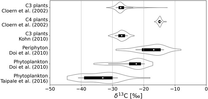
FIGURE 1. Ranges of δ¹³C values observed in C3 and C4 plants, in phytoplankton and in benthic algae (periphyton) in previous studies. In each distribution, the white dot indicates the median, the thick black bar indicates the interquartile range, the thin black line indicates the range of values between the 10- and 90-percentiles, and the wavy curves indicate the Gaussian kernel density estimate of the distribution of values.

An important methodological requirement for studies using δ¹³C to investigate C cycling in lakes is to determine a reference δ¹³C-CH₄ value for the source of CH₄, sometimes referred to as the endmember δ¹³C signal representative of the CH₄ produced in the sediments. Just as the enzyme systems involved in methanogenesis discriminate strongly against ¹³C, this is also the case for enzymatic reactions by methanotrophic microorganisms leading to MOX. As a result, the pool of CH₄ that remains after being exposed to MOX gradually gets more enriched in ¹³C (i.e., δ¹³C-CH₄ becomes less negative) the greater proportion is oxidized while CO₂ and microbial biomass formed by MOX get more ¹³C depleted. Accordingly, the difference between endmember δ¹³C-CH₄ and δ¹³C of partially oxidized CH₄ pools can be used to estimate the fraction of the original CH₄ being oxidized. In addition, δ¹³C measured in C pools can be compared to the source δ¹³C-CH₄ to estimate the fraction of C that has a methanogenic origin. Therefore, δ¹³C analyses are very useful to quantify complex ecosystem processes involving CH₄ from measurements of limited numbers of samples. However, the success of this approach critically depends on accurate and reliable knowledge of the relevant endmember δ¹³C-CH₄ values.

Several factors can affect the endmember δ¹³C-CH₄ in sediments of lakes. One is the bacterial community composition, and more specifically the share of different methanogenic pathways that are active (Conrad, 2005). The two main methanogenic pathways are based on CO₂ reduction (hydrogenotrophic methanogenesis; HM) and acetate dependent (acetoclastic methanogenesis; AM), and different enzyme systems can fractionate (i.e., discriminate) differently against ¹³C. A second aspect is the δ¹³C composition of the substrates used by methanogens (Conrad, 2005). This applies to organic substrates, and to the CO₂ or dissolved inorganic C (DIC) used in HM (dissolved CO₂ is connected to the whole DIC pool via the carbonic acid chemical equilibrium system). Bacterial communities and substrate composition differ from one lake to another, leading to varying δ¹³C-CH₄ endmember values in different systems (Rinta et al., 2015).

Recent results from a few subarctic lakes also indicate pronounced differences in endmember δ¹³C-CH₄ within lakes, e.g., between littoral and profundal regions (Cadieux et al., 2016; Thompson et al., 2016; Wik et al., 2020). Such variability would have important implications for the applicability of the δ¹³C approach to trace CH₄-related C cycling but has rarely been investigated systematically across different lake types and it is not clear if the observed patterns are widespread and consistent features of lakes or specific to the few subarctic systems studied so far. In this study, we compare δ¹³C-CH₄ values in littoral sediments, where the water was approximately 1 m deep, and in the deep, anoxic hypolimnion in the profundal zone, representing commonly used endmembers for estimation of MOX near the oxyclines of sediments or water columns, of six boreal lakes with different characteristics. We also carry out more detailed studies of one of the lakes where information about CH₄ input via groundwater (GW) from an adjacent mire could be generated. We hypothesize that δ¹³C-CH₄ values in deep, anoxic water are more negative than in littoral sediments, as previous observations mentioned above have shown, but that the magnitude of the difference increases in lakes with higher contrasts in the composition of OM reaching littoral and profundal sediments.

2 Materials and Methods

2.1 Study Sites

Samples were collected in six lakes across Sweden during the ice-free season in 2017, 2018, and 2019 (see Table 1 for their characteristics). STJ, LJR, and NAS are small lakes, located in the same region in the north of Sweden, that cover a range of dissolved organic C (DOC) levels. They are surrounded by coniferous forests (Scots pine and Norwegian spruce) with some presence of birch. Human activities around these lakes are connected to forestry. PAR and VEN are located in the southeastern part of Sweden. PAR is a small humic lake surrounded by a forest where Scots pine and Norwegian spruce dominate, and birch is also present. VEN is a relatively big and eutrophic lake. It is surrounded by some forested areas and agricultural land. SGA is a middle-size, deep, and clear lake located in the southwestern part of Sweden. It is surrounded by forests with a majority of Scots pines and Norwegian spruces and some birches.

TABLE 1

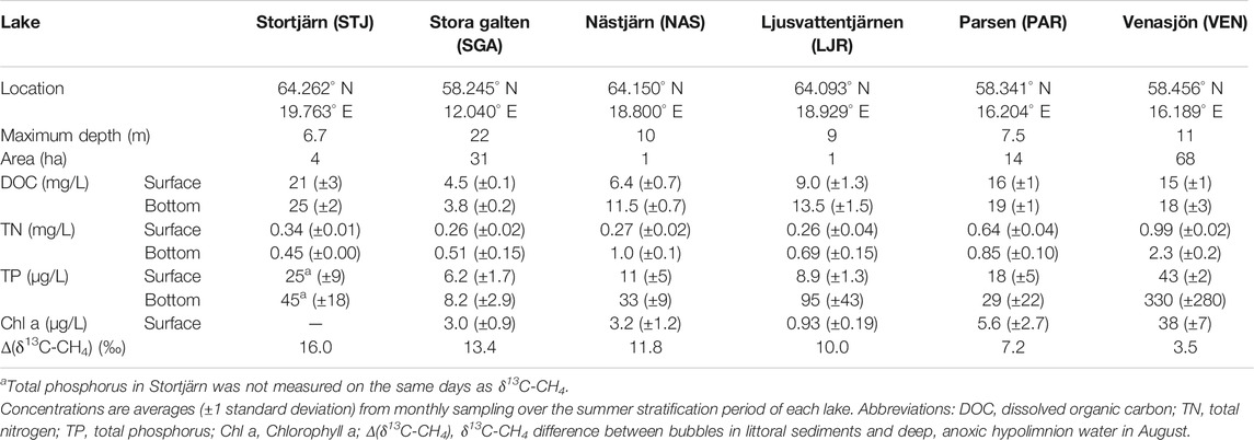
TABLE 1. Characteristics of the lakes investigated in the present study.

All lakes were sampled monthly during the summer stratification period (except STJ, where sampling was conducted several times but only in August) after some CH₄ had accumulated in anoxic parts of the water column close to the bottom to ensure a minimum influence of MOX on the deep water CH₄ sampled.

2.2 Sampling and Analyses Common to All Lakes

2.2.1 δ¹³C Values of CH₄

The δ¹³C-CH₄ at the bottom of the lakes was measured in anoxic water less than 1 m above the sediments, near the deepest point of each lake. A possibility exists that δ¹³C values measured in dissolved CH₄ in the water column above the sediments differ from δ¹³C-CH₄ values in the sediment bubbles if anaerobic oxidation of CH₄ (AOM) occurs at the interface between sediments and water column. However, the net effect of AOM would be to increase δ¹³C-CH₄ values in the water overlaying the sediments compared to δ¹³C-CH₄ values in the sediments themselves (Rinta et al., 2015; Marcek et al., 2021). Therefore, using our initial assumption that δ¹³C-CH₄ values are lower in the deep water of the profundal zone than in littoral sediment bubbles, differences in δ¹³C-CH₄ values between littoral sediment bubbles and dissolved CH₄ at the bottom of the water column provide a conservative estimate of the difference in δ¹³C-CH₄ values between profundal and littoral sediment bubbles.

Headspace extraction was used to collect δ¹³C-CH₄ samples from the deep water. Three methods were applied for the extraction. A first method consisted of sampling water at a given depth using a plastic Ruttner-type water sampler equipped with a tubing at the bottom. The water was then transferred to a 1.2 L plastic bottle by inserting the tube of the water sampler down to the bottom of the bottle. To prevent the build-up of air bubbles in the bottle and the exchange of gas between the water and the air during the transfer, the bottle was overflown with 2 L of water. The bottle was then closed with a rubber stopper equipped with two tubes attached to three-way luer-lock valves on the outside. A headspace was created in the bottle by injecting 60 ml of synthetic air containing only molecular nitrogen (N₂), O₂ and argon, and by simultaneously retrieving 60 ml of water through the tubes. The synthetic air used for the headspace was the same as the gas used as carrier by the instrument on which these samples were analyzed (see below). The bottle was then shaken manually for 3 min to equilibrate the gas in the water with the newly created headspace. Finally, the equilibrated gas in the headspace was retrieved from the bottle using a 60 ml syringe (Becton Dickinson, Franklin Lakes, New Jersey, United States) and transferred to a glass vial capped with a 10 mm butyl rubber stopper. The vial was manually evacuated using another 60 ml syringe right before transferring the sample. The residual CH₄ concentration in the vial after evacuation did not affect the measured δ¹³C-CH₄ because of the high CH₄ concentration in samples stored in manually evacuated vials (concentrations in the vials ranged between 76 ppm and 137000 ppm, and the residual gas only contained atmospheric CH₄ concentration). Also, the presence of O₂ in the vial did not cause CH₄ to be oxidized because only gas and no water was injected. Upon sample injection in the vial, an overpressure was created in the vial by injecting a larger volume of gas than the volume of the vial. A second extraction method consisted of sampling 60 ml of water at a given depth either through a long tube attached to a weight and connected to a 60 ml syringe at the surface, or by transferring water collected with the Ruttner sampler to a 60 ml syringe. Water was then transferred from the syringe to a 118 ml vial that had been flushed, filled with N₂, and amended with 0.2 ml of 85% H₃PO₄ prior to sampling. The acid was added because the vials were also used to collect samples for DIC, and to prevent biological production and oxidation of CH₄ in the vials. When prefilling the vials with N₂ an overpressure was created, which was released just before injecting the sample. Thereby, the total pressure of the vial headspace after sample injection could be calculated from the total barometric pressure when sampling, the sample volume, and temperature, and the equilibrated headspace constituted the gas sample analyzed. The third extraction method consisted in collecting 30 ml of water and 30 ml of air in a 60 ml syringe. CH₄ was extracted from the water to the headspace by shaking the syringe for at least 1 min and the headspace air was transferred to a manually pre-evacuated vial. When using this method, a sample of atmospheric air was taken separately to correct for the effect of atmospheric CH₄ on the concentration and δ¹³C-CH₄ in the sample extracted from the water.

Bubbles from littoral sediments were collected on the same days as deep-water samples. Locations where bubble samples were taken were not always similar among sampling occasions in each lake. The sampling procedure consisted in holding a plastic funnel connected to a 60 ml syringe upside down under water, physically disturbing the sediment under the funnel, and collecting released bubbles in the funnel syringe as they rose towards the surface. The collected gas was injected to a manually pre-evacuated vial (12–30 ml). Enough gas was transferred to the vial to create a minimum of 10 ml overpressure.

δ¹³C-CH₄ samples were analyzed on a cavity ring-down spectrometer (G2201-I Isotopic Analyzer, Picarro, Santa Clara, California, United States). Samples with high concentration of CH₄ were diluted with high purity synthetic air (80% N₂ and 20% O₂) to fall in the optimal range of concentrations for the instrument. To correct for non-linearity and guarantee the accuracy of the measurements in this range of concentrations, calibration curves were derived from the analysis of two standards with δ¹³C-CH₄ values of −66.5 ± 0.2‰ and −23.9 ± 0.2‰ (Isometric Instruments, Victoria, British Columbia, Canada), that were diluted to 20–25 different concentrations ranging logarithmically from 1 to 200 ppm CH₄. All values obtained after the analysis were corrected according to the calibration curves.

2.2.2 Water Chemistry

In all lakes except for STJ, where water chemistry is routinely monitored by the research station managing the site, water samples for DOC, DIC, total nitrogen (TN), total phosphorus (TP), and Chlorophyll a (Chl a) analysis were collected on the same days as the δ¹³C-CH₄ samples. Water was collected near the deepest point of each lake at 1 m depth and 1 m above the sediments using a Ruttner sampler equipped with a tubing at the bottom. For each depth, water was transferred to one 4 L cubitainer for DOC, DIC, TN, and Chl a analysis and two 125 ml HDPE bottles for TP analysis. The samples were kept in cooling boxes in the field. Within the same day as collection, a part of the water from the cubitainers was directly transferred to 50 ml PP tubes (Sarstedt, Nümbrecht, Germany) and stored at 4°C for subsequent TOC and TN analysis. Another part of the water from the cubitainers was filtered using pre-combusted 0.7 µm pore size grade GF/F filters (Whatman, Maidstone, United Kingdom) and the filtrate was stored in 50 ml PP tubes at 4°C for subsequent DOC and DIC analysis. The remaining water was filtered using 1.2 µm nominal pore size grade GF/C (Whatman) filters that were frozen immediately after filtration for storing them until subsequent Chl a analysis.

DOC, DIC, and TN samples were analyzed with a TOC/TN analyzer (Shimadzu, Kyoto, Japan). Samples containing more than 20 mg TOC/L were diluted with deionized water before analysis. Standard samples containing 10 mg TOC/L and 1, 2 or 5 mg TN/L were also analyzed and were used to correct the results from the lake samples. TP samples were analyzed on a continuous flow analyzer (AutoAnalyzer II, Bran + Luebbe) according to the AutoAnalyzer method no. G-175-96 Rev. 16 based on Murphy and Riley (1962). Chl a was extracted from the GF/C filters in methanol and measured by spectrophotometry following the Swedish Standard SS 28170, which is based on Richards and Thompson (1952).

Based on the measured concentrations of DIC, a value expressing the relative contribution of respired C to the DIC pool in the hypolimnion, the hypolimnetic excess DIC, was calculated as:

$Hypo\mathit{lim}neticexcessDIC=\frac{DI{C}_{bottom}-DI{C}_{surface}}{DI{C}_{surface}}(2)$

where DIC_bottom and DIC_surface are the concentrations of DIC at the bottom and surface of the lake, respectively.

2.3 Extended Sampling and Analyses in Stortjärn

At STJ extended sampling was carried out warranting additional description. STJ is located in the Krycklan Catchment Study area in northern Sweden (Laudon et al., 2013). The lake has a maximum and mean depth of 6.7 and 2.7 m, respectively (Denfeld et al., 2018). It is separated in two main basins along a north-south axis, the western basin being about half the size of the eastern basin (Figure 2). More than half of the shoreline of the lake is covered by a Sphagnum mire (Figure 2). The lake catchment has as surface area of 65 ha and is composed at 39.5% of wetland and at 54% of forest (Figure 2; Laudon et al., 2013). The main types of soils in the catchment are till deposits covered locally by thin forest soil and peat. Average yearly precipitation in the catchment is 614 mm (Laudon et al., 2013).

FIGURE 2

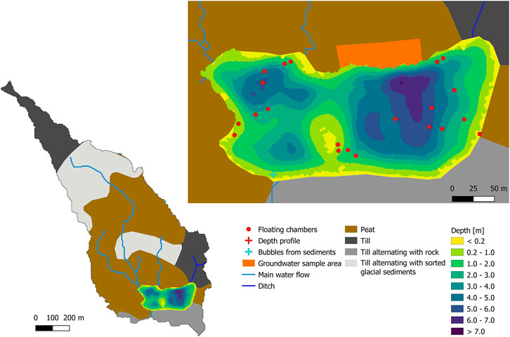
FIGURE 2. Left: Types of soil and theoretical water flow direction in the catchment of Stortjärn. The outlet of the lake is located at the southwestern shore. The water flow direction in the mire on the northwestern side of the lake is calculated based on the DEM of the catchment. A small ditch forms a small inlet in the northeastern corner of the lake. Right: Bathymetric map of the lake with locations where groundwater, water column depth profiles and bubbles in littoral sediments were sampled, and positions of the floating chambers used to measure CH₄ fluxes at the surface of the lake. ^©Lantmäteriet, i2012/901.

The additional mapping of lake CH₄ fluxes of relevance carried out in STJ included water samples taken in the mire to measure δ¹³C-CH₄ in the GW, measurements of daily CH₄ emissions at the water-atmosphere interface of the lake using floating chambers, and estimation of daily input of CH₄ from the mire using a water balance of the lake.

2.3.1 CH₄ Concentration in the Water

Water samples for CH₄ concentration were collected using a 10 ml plastic syringe (Becton Dickinson). After rinsing the syringe, 5 ml of water were collected at 10 cm depth making sure that no air bubble was introduced in the syringe. The water was transferred to a 22 ml vial capped with a butyl rubber stopper that had been amended with 0.1 ml of 85% H₃PO₄ for sample preservation and then flushed and filled with N₂ prior to sampling. The vials were prepared with a N₂ overpressure that was released just prior to injecting the water sample to equilibrate the pressure towards the present barometric pressure and ensure that vials did not leak before used for samples. The concentration of dissolved CH₄ in the water was calculated from the sum of 1) the CH₄ content in the vial headspace measured with gas chromatography (GC System 7890A with a 1.8 m × 3.175 mm Porapak Q 80/100 column from Supelco, a methanizer and a flame ionization detector, Agilent Technologies, Santa Clara, California, United States) and determined using the common gas law, and 2) remaining CH₄ dissolved in the water in the vial determined from headspace concentration using Henry’s law and the temperature adjusted Henry’s solubility constant for CH₄ in freshwater.

2.3.2 CH₄ Emissions to the Atmosphere

The rate of CH₄ emissions at the lake’s surface was measured at different locations using flux chambers (Bastviken et al., 2004). These flux chambers were made of plastic buckets (6 L, 800 cm² opening area) equipped with floats and placed at the surface of the lake. The flux of CH₄ between the surface water and the atmosphere was determined by measuring the change in CH₄ concentration in the chamber over time. Each chamber was attached to a separate float connected to an anchor to allow the chambers to move freely with waves and water level changes. When chambers were deployed, atmospheric air samples and surface water samples were collected near some of the chambers. Atmospheric air samples taken 20 cm above the surface of the water were used to represent initial concentration in the chambers. Surface water samples were collected as described previously. After a deployment period, each chamber headspace was sampled through a polyurethane tube (5 and 3 mm outer and inner diameter, respectively) equipped with a three-way luer-lock valve. These samples were collected prior to redeploying the chambers to start a new measurement cycle. The deployment period of the chambers ranged from 4 to 48 h during the sampling period. Note that CH₄ was highly supersaturated in the studied lakes and that equilibration with chambers therefore took much longer than 48 h—in contrast to CO₂ which typically equilibrates in flux chambers within a few hours and therefore demands much shorter chamber deployments than CH₄. Samples of gas from the chambers and of ambient air were collected using three 60 ml syringes for having a total volume of 180 ml of gas. They were transferred to 22 ml vials with butyl rubber stoppers. Each vial was flushed using 165 ml of the collected gas. The remaining 15 ml of gas were added after removing the gas outlet needle from the vial stopper, creating an overpressure in the vials. All CH₄ gas samples were analyzed with gas chromatography as above. The overpressure in the vials containing the samples was checked as a leakage indicator and was released to equilibrate vials with atmospheric pressure just before the analysis.

2.3.3 δ¹³C-CH₄ in Groundwater

GW samples for δ¹³C-CH₄ analyses were collected in the mire on the north side of STJ with the use of piezometers (Figure 2). GW samples were collected at different distances from the lake and at 1 m depth in the mire. After discarding the water that was trapped in the tubing, 60 ml of water were collected using a 60 ml syringe. This water was transferred to a 118 ml vial prepared as explained in the description of the second method used to collect δ¹³C-CH₄ water samples.

2.3.4 Weather Variables and Depth Profiles

Air temperature, relative humidity, barometric pressure, and wind speed were measured by a weather station located on a platform in the center of the lake. Data were averaged and logged every 10 min. Daily precipitation data were provided by a rain gauge located 2 km away from the lake. Water temperature was logged every 10 min by sensors positioned every 25 cm from the surface to the bottom of the lake at the platform where weather parameters were measured. The water level in the lake was averaged and logged every 10 min. Daily discharge in the outlet of the lake was measured at a V-notch weir located 30 m downstream of the lake.

2.3.5 Flux Calculation

CH₄ fluxes at the surface of the lake were measured using the method described in Bastviken et al. (2004). The calculation of diffusive flux relies on Fick’s law of diffusion:

$F=k\left(C_w-C_{fc}\right)(3)$

where F is the flux of CH₄ across the water-air interface (mmol m⁻² d⁻¹), k is the piston velocity (m d⁻¹), C_w is the concentration of CH₄ in the surface water (µmol L⁻¹) and C_fc is the calculated equilibrium concentration of CH₄ in water corresponding to the flux chamber headspace concentration (µmol L⁻¹). Using this equation and measurements of C_w and C_fc after some time, k is solved for by accounting for the gradual change in flux due to the increasing C_fc over time, i.e., using a non-linear regression over the measurement cycle as described in Bastviken et al. (2004). Then, k for chambers receiving only diffusive flux (see below) was used with C_w to estimate instantaneous diffusive flux, setting C_fc to the initial air background CH₄ level.

Floating chambers accumulate CH₄ emitted by both diffusion and ebullition. Their relative contribution to the measured total flux is estimated based on the method given in Bastviken et al. (2004). The values of k derived for different chambers from the measured flux and water concentrations during the same period were divided by the minimum k value observed for this period. Chambers for which this k ratio was below a certain threshold [we used a threshold of 2 in this study based on independent findings in Bastviken et al. (2004); Schilder et al. (2013)] were assumed to receive CH₄ only by diffusion. Therefore, it was assumed that the diffusive part of the flux is rather homogeneous across the lake surface (within the 2-fold variability on k combined with variability on C_w) and that not all chambers collect CH₄ bubbles. The contribution of ebullition in the chambers where the k ratio was above the threshold was calculated by subtracting the average flux from the chambers collecting only diffusive flux from the total flux of each chamber.

2.3.6 Water Balance and Lateral CH₄ Input

The water balance is used here to estimate the potential lateral input of CH₄ to STJ, which can be approximated by the volume of water flowing to the lake multiplied by the concentration of CH₄ in this water. The water balance of the lake expressed for the inflow of water to the lake is:

$Inflow= Outflow+E+A\Delta h-P_{lake}(4)$

where Inflow is the total amount of water entering the lake from the catchment, Outflow is the water leaving the lake in the outlet, E is the evaporation at the lake surface, A is the surface area of the lake, ∆h is the water level change in the lake and P_lake is the precipitation falling directly in the lake. The surface area of the lake was assumed to be constant over the range of water level changes. Evaporation was calculated according to Sartori (2000). All terms on the right-hand side of the equation could be calculated from parameters measured routinely in or around the lake.

To estimate the lateral CH₄ input to the lake, we assume that the water input is primarily in the form of GW flowing through the mire. This assumption is supported by the catchment distribution (Figure 2), the absence of any stream inlet to STJ, except for a small ditch in the northeastern corner of the lake, and the negligible input of CH₄ with GW from the forested shoreline, confirmed by previous measurements of GW CH₄ (Denfeld et al., 2020).

3 Results

3.1 δ¹³C-CH₄ in Anoxic Hypolimnion Water Versus Near-Shore Sediment Bubbles

In four lakes (STJ, SGA, NAS, LJR), the δ¹³C-CH₄ in the anoxic hypolimnion ranged from −80‰ to −76‰ during the measurement period (Figure 3). SGA is deep and oligotrophic, whereas the other three lakes are small and moderately to highly humic. By contrast, in PAR, which is also a humic lake located farther south but with higher TN concentrations and potential influence from more nutrient rich soils, δ¹³C-CH₄ at the bottom ranged between −75‰ and −73‰. In VEN, a relatively large and eutrophic lake, the corresponding values ranged between −71‰ and −69‰. In all lakes, δ¹³C-CH₄ values from littoral sediments ranged between −71‰ and −58‰, except for LJR where lower values of −78‰ to −72‰ were observed between June and August. In the second half of August, when lakes were likely to have been stratified for an extended period and the only time when data was available for all lakes, the difference between δ¹³C-CH₄ measured in the littoral sediment bubbles and in the anoxic hypolimnion water (Δ(δ¹³C-CH₄)_LSB-AHW) was 16.0‰ in STJ, 13.4‰ in SGA, 11.8‰ in NAS, 10.0‰ in LJR, 7.2‰ in PAR, and 3.5‰ in VEN (Table 1). δ¹³C-CH₄ was lower in the anoxic hypolimnion than in the littoral sediments in all six lakes investigated (Figure 3).

FIGURE 3

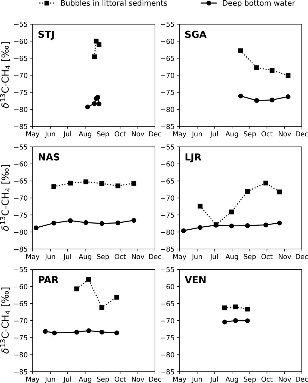
FIGURE 3. δ¹³C-CH₄ in the anoxic water close to the bottom at the deepest point (dots with continuous lines) and in the bubbles in littoral sediments (squares with dotted lines) in six lakes.

Δ(δ¹³C-CH₄)_LSB-AHW showed a tendency to decrease with increasing surface water concentration of TP if considering all times where both these variables were available (Figure 4). This tendency is partly a result of clearly lowest Δ(δ¹³C-CH₄)_LSB-AHW in the most nutrient rich lake VEN. In addition, some lakes showed decreasing Δ(δ¹³C-CH₄)_LSB-AHW with increasing TP when comparing different sampling times within the same lake (Figure 4). More generally, TP may not be an optimal indicator of lake productivity, e.g., as TP can be bound to DOC in humic boreal lakes, but we also observe that the two lakes with the smallest Δ(δ¹³C-CH₄)_LSB-AHW in August (VEN and PAR), presumably reflecting the integrated result of the summer productivity, had highest TP, TN, and Chl a levels (Table 1).

FIGURE 4

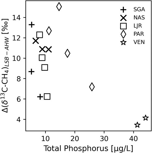
FIGURE 4. Difference in δ¹³C-CH₄ between littoral sediment bubbles (LSB) and anoxic hypolimnion water (AHW) compared to total phosphorus concentration in surface water in the middle of each lake. Each point corresponds to 1 day when both δ¹³C-CH₄ and total phosphorus were sampled.

We also observed that δ¹³C-CH₄ in the anoxic, hypolimnetic water was lower in lakes with higher hypolimnetic excess DIC (defined in Eq. 2; Figure 5A). In VEN, where DIC concentrations were relatively homogeneous over the water column (hypolimnetic excess DIC = 1–2), the δ¹³C-CH₄ values at the bottom were around −70‰ (Figure 5A). PAR was an intermediate case with hypolimnetic excess DIC of 2–4 and bottom δ¹³C-CH₄ values between −73‰ and −74‰ (Figure 5A). The other lakes all had hypolimnetic excess DIC of 3–10 and bottom δ¹³C-CH₄ values between −76‰ and −80‰ (Figure 5A). However, no particular relation between Δ(δ¹³C-CH₄)_LSB-AHW and hypolimnetic excess DIC could be observed (Figure 5B).

FIGURE 5

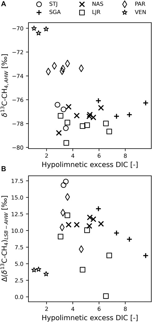
FIGURE 5. (A) δ¹³C-CH₄ in anoxic hypolimnion water (AHW) compared to the hypolimnetic excess dissolved inorganic carbon (DIC), calculated as the difference in DIC concentration between bottom and surface water normalized by the concentration at the surface. (B) δ¹³C-CH₄ difference between AHW and littoral sediment bubbles (LSB) compared to the hypolimnetic excess DIC. In both panels, each point corresponds to 1 day when both δ¹³C-CH₄ and DIC were sampled.

Overall, it was clear and consistent across all lakes that bottom anoxic water δ¹³C-CH₄ was more negative (more depleted in ¹³C) than littoral CH₄ bubbles, with indications of possible links to lake productivity (here estimated via proxies), and a proxy for in lake respiration (hypolimnetic excess DIC).

3.2 Possible Groundwater Influence on CH₄ in Lake Stortjärn

The δ¹³C-CH₄ values measured in the surface water of STJ ranged between −57.2‰ and −47.4‰ with an average of −53.6‰ (Figure 6). In the bubbles collected in the littoral sediments, δ¹³C-CH₄ ranged between −64.9‰ and −58.9‰ with an average of −62.6‰ (Figure 6). In the GW, δ¹³C-CH₄ ranged between −81.4‰ and −70.1‰ with an average of −76.2‰ (Figure 6). The water samples taken at different depths at the deepest point of the lake show that δ¹³C-CH₄ decreased with depth. The average value was −56.2‰ between 0 and 1.5 m and went down to −76.8‰ at depths below 3 m (Figure 6).

FIGURE 6

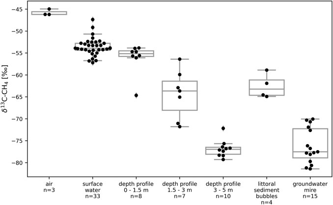
FIGURE 6. Boxplots and individual measurements of δ¹³C-CH₄ values in the air, in lake water (surface and depth profiles) and littoral sediments, and in the mire groundwater in Stortjärn in August. “Surface water” data represents spatial variability at the surface of the lake while “depth profile” data shows short term variability at different depths in the central part of the lake. Figure 2 shows a map with all sampling locations. Boxes extend from the lower quartile to the upper quartile. Whiskers extend to the nearest measurements within bounds corresponding to one and a half time the width of the boxes.

Precipitation measurements in the catchment of the lake and the water budget of the lake show that three major rain events occurred during the sampling period, each lasting between one and 2 days and releasing decreasing amounts of water to the lake over several days after each rain event. The daily input of CH₄ from the mire to the lake was calculated by multiplying the daily water inflow from the mire with the average concentration of CH₄ that was measured in the GW of the mire (178 µM; very close to the average concentration measured in the same mire over the entire ice-free period in another study; Denfeld et al., 2020). The daily input of CH₄ from the mire ranged from 0.14 to 6.8 kg CH₄ with an average of 1.6 kg CH₄ (Figure 7).

FIGURE 7

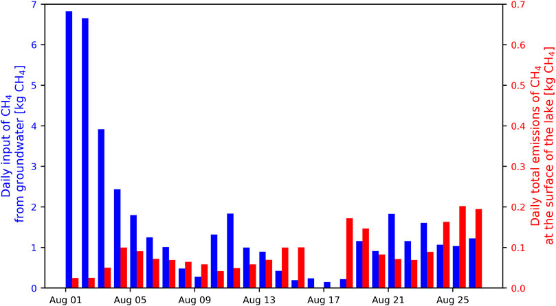
FIGURE 7. Comparison between the estimated daily input of CH₄ from the mire to Stortjärn (blue bars) and the total amount of CH₄ emitted each day at the surface of the lake (red bars; note the tenfold difference between left and right y-axes scales). Emissions of CH₄ at the surface of the lake were not measured on 16–17 August.

Fluxes of CH₄ measured at the surface of the lake ranged between 0.01 and 64 mg CH₄ m⁻²d⁻¹, with mean and median values of 2.9 and 1.4 mg CH₄ m⁻²d⁻¹, respectively. Daily whole-lake emissions of CH₄, calculated as the average of all chamber measurements for each day multiplied by the surface area of the lake, ranged from 24 g CH₄ to 200 g CH₄ with an average of 90 g CH₄. Flux rates were one to two orders of magnitude smaller than the calculated daily CH₄ input from the mire (Figure 7).

4 Discussion

4.1 δ¹³C-CH₄ in Anoxic Hypolimnion Water Versus Near-Shore Sediment Bubbles

The thermal stratification in the lakes resulted in typical depth profiles of CH₄ concentrations and δ¹³C-CH₄ values, with low CH₄ concentrations and high δ¹³C-CH₄ values in the oxic epilimnion, and high CH₄ concentrations and low δ¹³C-CH₄ values in the anoxic hypolimnion. The δ¹³C-CH₄ values we observed in the anoxic hypolimnion of all six lakes are in the same range as observations previously reported in other lakes (Rinta et al., 2015; Thompson et al., 2016). Our results also show that CH₄ was more ¹³C enriched in littoral sediment bubbles of all six lakes than in anoxic water in the hypolimnion (Figure 3). Considering that CH₄ in profundal sediment bubbles would most likely be more δ¹³C depleted than in the overlaying water column (Rinta et al., 2015; Marcek et al., 2021), particularly in cases where significant AOM occurs, it implies that even larger differences in δ¹³C values than the ones we observed can be expected between CH₄ in profundal and littoral sediment bubbles. Lower δ¹³C-CH₄ values in the profundal compared to the littoral zones have also been observed in sediments of three small subarctic lakes in western Greenland (Cadieux et al., 2016; Thompson et al., 2016) and in one small subarctic lake located on the border of a permafrost complex in northern Sweden (Wik et al., 2020). However, as such studies were made on a limited number of lakes with similar properties, it was unclear whether such differences in endmember δ¹³C-CH₄ are common across lakes. Our results indicate that patterns of highly variable endmember δ¹³C-CH₄ values, but with a consistent difference between littoral and profundal zones is a common property of boreal and subarctic lakes. This observation is critical for how to use and sample δ¹³C-CH₄ values to assess CH₄ cycling, MOX, and other related lake ecosystem processes or food web interactions.

It is also remarkable that δ¹³C-CH₄ values in the anoxic hypolimnion water were relatively similar among sampling occasions in all lakes while littoral sediment δ¹³C-CH₄ values were more variable. The variability was observed as variability over time but could in fact also represent variability in space because sediment bubbles were not collected at identical locations every time and the temporal variability was asynchronous between lakes, even in similar lakes like NAS and LJR. This means that local conditions in the littoral sediments, for example sources of organic matter, benthic processes, and vegetation cover, can vary in ways that could influence endmember δ¹³C-CH₄ signals substantially.

4.2 Possible Explanations for Observed Patterns

We discuss below a range of potential explanations for the difference in δ¹³C-CH₄ we observed between littoral sediment bubbles and the anoxic hypolimnion.

4.2.1 Substrates for Methanogenesis

Δ(δ¹³C-CH₄)_LSB-AHW can be related to differences in δ¹³C of the substrates used in the anoxic degradation of OM in sediments of lakes. δ¹³C-CH₄ is determined by the initial δ¹³C of the substrate and by the fractionation imposed by metabolic reactions, such that δ¹³C of the substrate plays an important role in setting δ¹³C of CH₄ released in the water column (Conrad, 2005). The dominant sources of OM to the sediments of lakes include autochthonous primary production by phytoplankton, benthic algae, or littoral vascular plants on one hand, and allochthonous terrestrial OM on the other hand. Terrestrial OM is derived from the vegetation growing in the catchment of the lake, which is predominantly constituted of C3 plants in boreal regions (Cerling et al., 1997). δ¹³C for C3 plants are typically between −37‰ and −20‰ and most commonly near −27‰ (Kohn, 2010). In general, values of −27‰ or −28‰ are commonly used for allochthonous C in boreal lakes (Meili et al., 1993; Pace et al., 2004). δ¹³C values of littoral vascular plants are also predominantly in the range between −30‰ and −20‰ (Cloern et al., 2002; Lammers et al., 2017; Figure 1). On the other hand, δ¹³C values for different phytoplankton species have been reported in the range −44.5‰ to −18‰ in several boreal lakes, most of them being in the range −39‰ to −30‰ (Taipale et al., 2016), and measurements in several lentic systems across a broad range of latitudes have revealed δ¹³C values ranging between −36‰ and −17‰ in phytoplankton and between −29‰ and −8‰ in benthic algae, with values usually 2‰–11‰ lower (6‰ in average) in phytoplankton than in benthic algae for a given system (Doi et al., 2010), as illustrated in Figure 1. Therefore, benthic algae seem usually enriched in ¹³C compared to phytoplankton and allochthonous OM. There are indications that methanogens preferentially use autochthonous freshly produced OM when possible (West et al., 2012).

Hence, in low-nutrient lakes, the littoral where light is available may represent a zone with concentrated production of fresh, autochthonous OM (Karlsson et al., 2009). Nutrients released from sediments may be the main nutrient source in such low-nutrient lakes, favoring benthic algae relative to phytoplankton. If so, littoral δ¹³C-CH₄ in low-nutrient lakes may be influenced by benthic algae, while profundal CH₄ production is reflecting δ¹³C from allochthonous OM (or respired DIC as discussed further below), which given this scenario could lead to a large Δ(δ¹³C-CH₄)_LSB-AHW. In more nutrient rich lakes, settling phytoplankton may contribute labile autochthonous OM fueling methanogenesis everywhere in the lake (in both littoral and profundal sediments) leading to lower Δ(δ¹³C-CH₄)_LSB-AHW. The wide range of δ¹³C values in phytoplankton reported in previous studies (Doi et al., 2010; Taipale et al., 2016) and illustrated in Figure 1 does not necessarily contradict this explanation, as measured δ¹³C-CH₄ values reflect average δ¹³C values in the sediments, and the mean δ¹³C value in phytoplankton is significantly lower than the mean δ¹³C value in benthic algae (Wilcoxon signed-rank test on the data from Doi et al. (2010); N = 49, W = 1.0, p < 0.001). However, the wider range of phytoplankton δ¹³C values can add to the variability among lakes. Although the substrate explanation is a speculation at this stage it is realistic given available scientific evidence and could explain our observations of lower Δ(δ¹³C-CH₄)_LSB-AHW in lakes with highest TP, TN, and Chl a values (Table 1).

In addition, DIC is the C substrate for HM, and it is possible that DIC in profundal sediments under isolated hypolimnion is primarily generated by OM respiration which causes depletion in ¹³C compared to DIC in littoral parts of lakes where continuous exchange with atmospheric CO₂ is possible (Miyajima et al., 1997; Karlsson et al., 2007). A few measurements in the lakes studied here confirm this tendency and indicate that δ¹³C-CO₂ at the bottom of the water column is often between 2‰ and 10‰ lower than in surface water (data not shown). Therefore, δ¹³C values of CH₄ produced by HM should decrease at the bottom of lakes with larger differences between bottom and surface DIC concentrations (expressed as hypolimnetic excess DIC in the Results) being a sign of a larger share of accumulated respired C in deep waters. Accordingly, we observed the most positive hypolimnion δ¹³C-CH₄ values in VEN, which also had smallest DIC accumulation in deeper water. Comparing lakes with distinctively different δ¹³C-CH₄ values in the hypolimnion, we also noted that increasing hypolimnetic DIC accumulation was linked with lower δ¹³C-CH₄ values in the hypolimnion (Figure 5A). This indicates that some CH₄ was produced by HM in the hypolimnion of the studied lakes.

The subsequent question is if a depletion of δ¹³C-CH₄ from HM using respired C could explain the observed Δ(δ¹³C-CH₄)_LSB-AHW. If this was the case, we would expect larger Δ(δ¹³C-CH₄)_LSB-AHW when a greater share of respired C were present in the hypolimnion, i.e., we would expect a positive relationship between Δ(δ¹³C-CH₄)_LSB-AHW and the hypolimnion excess DIC. However, no such strong pattern could be observed (Figure 5B). Therefore, we conclude that while differences in types of OM substrates (terrestrial/macrophytes vs. phytoplankton vs. periphyton) could provide explanations, CH₄ production from respired C does not seem to be a main direct driver for the observed Δ(δ¹³C-CH₄)_LSB-AHW.

4.2.2 Pathways of Methanogenesis

If the balance between methanogenic pathways differs between littoral and profundal sediments, δ¹³C-CH₄ values could be affected because HM has been suggested to generate more depleted δ¹³C-CH₄ than AM (Whiticar, 1999). The lower δ¹³C-CH₄ values that we report in the deep hypolimnion compared to littoral sediments could then be explained if a greater share of HM is taking place in profundal sediments compared to littoral ones. Our data on δ¹³C-CH₄ and DIC measurements discussed above indicates that HM occurs and consumes respired CO₂ in the deep hypolimnion. While we do not have direct estimates of AM and HM, several factors influencing the share of CH₄ produced by HM and AM have recently been reviewed by Conrad (2020). They include temperature, pH, and the quality of the available OM. More specifically, previous observations have shown that the HM:AM ratio decreases at lower temperature (Schulz and Conrad, 1996; Nozhevnikova et al., 2007) while low pH values can limit the availability of H₂ resulting in a smaller contribution from HM (Goodwin et al., 1988). In addition, Liu et al. (2017) have shown that the HM:AM ratio increased in deeper layers of sediment cores from a mountain lake, which was explained by the decreasing quality of the OM in older sediments. Given present literature information, our data is not clearly compatible with conditions that would favor HM in profundal zones and AM in the littoral, as some variables such a temperature conditions could be expected to yield the opposite result. Hence, although this HM vs. AM hypothesis cannot be excluded as a potential explanation for our results, we find it unlikely that it is of main importance.

4.2.3 Partial MOX

A difference in rates of MOX in sediments across depths needs to be considered as a potential explanation for the spatial variability of δ¹³C-CH₄ because MOX leaves ¹³C enriched CH₄ by preferentially consuming lighter ¹²C-CH₄. More MOX is expected to happen in littoral sediments than in deep, anoxic hypolimnia as MOX in littoral sediments can be supported by the transport of suitable electron acceptors into the sediments via plant roots or via diffusion or percolation of O₂-rich water. However, if the collected bubbles in the littoral sediments were released from sediment layers below the zone where suitable electron acceptors for MOX or AOM were depleted, δ¹³C-CH₄ values measured in these bubbles would not have been affected by oxidation. Unfortunately, in the absence of measurements of δ¹³C-CH₄ profiles in the pore water of the sediments, it is not possible to confirm if this was the case in the present study. Measurements in a small, eutrophic kettle lake in central Europe, which included collection of sediment bubbles using a similar approach as the one described here, as well as profiles of pore water δ¹³C-CH₄, showed that bubbles released by physically disturbing the sediments originated from sediment layers where CH₄ was not or marginally affected by oxidation (Langenegger et al., 2019). If the same is true in the littoral and profundal sediments of the lakes studied here, it would indicate that MOX is not a likely explanation for the higher δ¹³C-CH₄ values observed in littoral sediment bubbles compared to in anoxic, deep water in the profundal zone of the lakes. Direct measurements of CH₄ concentrations and δ¹³C-CH₄ values along pore water profiles in the sediments in littoral and profundal zones could provide more conclusive results by allowing a more detailed analysis of the active processes in different sediment layers and should be included in future studies.

4.2.4 Groundwater Influence on CH₄ in Lake Stortjärn

GW often contains high concentration of CH₄ compared to lake water due to anoxic conditions prevailing in soils (Bugna et al., 1996). Moreover, GW can also be a significant source of CH₄ to some lakes (Einarsdottir et al., 2017; Lecher et al., 2017; Dabrowski et al., 2020). A previous study indicates that large amounts of CH₄ might be transported to STJ via GW inputs (Denfeld et al., 2020). The GW flowing into STJ passes through a mire and CH₄ emitted from wetlands and mires often displays δ¹³C-CH₄ values lower than −60‰ (Quay et al., 1988; Lansdown et al., 1992), especially in Scandinavian wetlands where average values are as low as −75‰ (Ganesan et al., 2018). Our measurements show that δ¹³C-CH₄ in GW from the mire (−82‰ to −70‰) matches δ¹³C in the dissolved CH₄ (−79‰ to −72‰) under the oxycline in the middle of the lake near the deepest point (Figure 6). The deep water δ¹³C-CH₄ in the profundal zone is at the same time different from littoral sediment bubble δ¹³C-CH₄ values that were measured on the opposite side of the lake (−65‰ to −59‰; Figure 6). Together with the fact that the GW is expected to enter the lake in the deeper layer due to its low temperature (higher density) compared to the epilimnion, it points to a possible mire GW origin of CH₄ in the deeper water layer of the lake. On the other hand, most of the littoral sediment bubbles CH₄ is probably derived from sediment CH₄ production and less influenced by the mire CH₄. The GW explanation might also apply to other lakes than STJ. Unfortunately, the absence of GW measurements near the five other studied lakes prevents us to establish any link between GW inputs of CH₄ depleted in ¹³C and the lower δ¹³C-CH₄ values observed in the anoxic hypolimnion of these lakes. Alternatively, the low δ¹³C-CH₄ values observed in the anoxic hypolimnion of STJ might also arise for other reasons described previously, like the variability in the composition of the substrate available in different zones of lakes. It is likely that the suggested mechanisms have a combined effect on the difference in δ¹³C values in endmember CH₄ between littoral and profundal zones of lakes.

Furthermore, the amount of CH₄ transported by GW to the lake was estimated to be much larger than the amount of CH₄ emitted by the lake to the atmosphere (Figure 7). It implies that large quantities of CH₄ can be transported from the mire to the lake and most of this CH₄ is oxidized in the lake before reaching the surface. It suggests that the importance of GW CH₄ contributions to lakes CH₄ cycling may have been underestimated. In fact, these observations indicate that GW CH₄ inputs could be high enough to sustain most dissolved CH₄ in some lakes—meaning that hypolimnetic CH₄ and episodic fluxes of dissolved CH₄ upon lake mixing would be attributed to GW CH₄, while ebullition is derived from intrinsically produced CH₄ from the lake sediments. These findings deserve further studies and illustrate that catchment processes and hydrological transport should be considered in assessments of factors controlling CH₄ cycling in lakes. Accurate and relevant estimates of the volume of various sources and sinks of water to and from a lake, and of the CH₄ concentration in each of these sources and sinks are important requirements for this method to be successful in assessing the contribution of external inputs of CH₄ to the lake. Also, the temperature of the groundwater entering a lake is critical in determining in which layer of the lake the groundwater will end up.

5 Conclusion

The main result of our study is that there seems to be a systematic difference in endmember δ¹³C-CH₄ between littoral sediments and anoxic profundal zones of subarctic and boreal lakes and that it is important to consider which parts of the lake CH₄ cycling can be represented by different source δ¹³C-CH₄ values. We also discuss potential explanations to the observed pattern (Figure 8) and argue that several mechanisms are likely to contribute at different degrees to the offset in endmember δ¹³C-CH₄ between littoral and profundal zones of lakes, with no conclusive evidence for one specific mechanism against all others based on our observations.

FIGURE 8

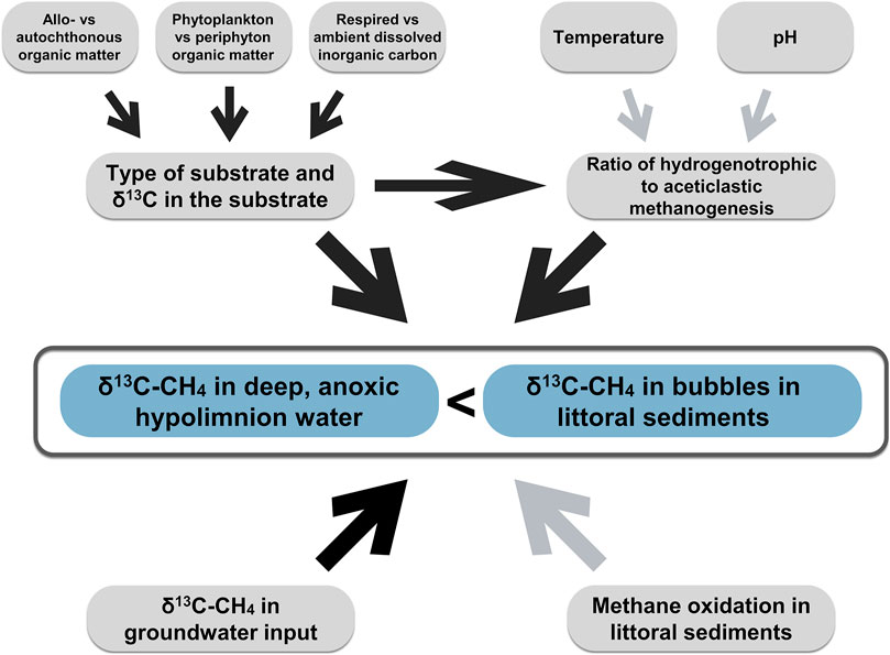
FIGURE 8. Conceptual figure summarizing the different processes discussed in the text as potential explanations for the observed variability in δ¹³C-CH₄ between the anoxic hypolimnion water and the littoral sediments of lakes. Dark arrows indicate relations supported by our measurements. Light arrows indicate relations that are not supported by our observations. See text for details.

It has been shown that stratified lakes in essence have two separated CH₄ cycles—one epilimnetic and one hypo-metalimnetic (Bastviken et al., 2008). In the epilimnetic CH₄ cycle, CH₄ produced in littoral sediments is released to the atmosphere by bubbling or diffuses into the epilimnion where it can be oxidized or emitted. The epilimnetic CH₄ cycle contributes most of the CH₄ emission during open water periods and the best source δ¹³C-CH₄ value there may be measured in littoral sediment bubbles. In the meta-hypolimnetic CH₄ cycle, CH₄ primarily leaves the profundal sediment as dissolved CH₄, and a concentration gradient develops between the surface of the sediments and the water layer where suitable electron acceptors for MOX are available and where most of the CH₄ is oxidized. For estimating MOX in this part of the lake, dissolved CH₄ in the anoxic bottom water layer of the lake or CH₄ contained in profundal sediments may be the best source δ¹³C-CH₄ value. Distinguishing these two CH₄ cycles would represent an important progress and contribute to increased knowledge about the regulation and feedbacks of lake CH₄ and C cycling and emissions.

Data Availability Statement

The datasets presented in this study can be found in online repositories. The names of the repository/repositories and accession number(s) can be found below: DiVA (https://doi.org/10.48360/5PPN-C440).

Author Contributions

The study was designed by HS, JS, and DB. Field work was performed by JS, HS, AS, GP, DR, EH, and KF. Sample analyses were performed by JS, HS, AS, GP, DR, EH, and KF. Funding for this study was provided through projects led by DB, HL, and JK. The article was drafted by JS with contributions from all authors.

Funding

This work was funded by the European Research Council (ERC) under the European Union’s Horizon 2020 research and innovation programme (Grant agreement No 725546; METLAKE), the Swedish Research Council (Grant No 2016-04829), FORMAS (Grant No 2018-01794), and the Knut and Alice Wallenberg Foundation (Grant No 2016.0083).

Conflict of Interest

The authors declare that the research was conducted in the absence of any commercial or financial relationships that could be construed as a potential conflict of interest.

Publisher’s Note

All claims expressed in this article are solely those of the authors and do not necessarily represent those of their affiliated organizations, or those of the publisher, the editors and the reviewers. Any product that may be evaluated in this article, or claim that may be made by its manufacturer, is not guaranteed or endorsed by the publisher.

Acknowledgments

We thank Ingrid Sundgren, Thanh Duc Nguyen, and Kim Lindgren for invaluable assistance, the Swedish Infrastructure for Ecosystem Science (SITES), the Skogaryd Research Catchment (SRC), and inhabitants at Stora Galten, Parsen, and Venasjön for valuable support, interest, and patience with our work.

References

Bastviken, D., Cole, J. J., Pace, M. L., and Van de Bogert, M. C. (2008). Fates of Methane from Different lake Habitats: Connecting Whole-lake Budgets and CH4emissions. J. Geophys. Res. 113:G02024. doi:10.1029/2007JG000608

CrossRef Full Text | Google Scholar

Bastviken, D., Cole, J., Pace, M., and Tranvik, L. (2004). Methane Emissions from Lakes: Dependence of lake Characteristics, Two Regional Assessments, and a Global Estimate. Glob. Biogeochem. Cycles 18:GB4009. doi:10.1029/2004GB002238

CrossRef Full Text | Google Scholar

Bastviken, D., Ejlertsson, J., Sundh, I., and Tranvik, L. (2003). Methane as a Source of Carbon and Energy for Lake Pelagic Food Webs. Ecology 84, 969–981. doi:10.1890/0012-9658(2003)084[0969:maasoc]2.0.co;2

CrossRef Full Text | Google Scholar

Bastviken, D. (2009). “Methane,” in Encyclopedia of Inland Waters. Editor G. E. Likens (Oxford: Academic Press), 783–805. doi:10.1016/B978-012370626-3.00117-4

CrossRef Full Text | Google Scholar

Bugna, G. C., Chanton, J. P., Cable, J. E., Burnett, W. C., and Cable, P. H. (1996). The Importance of Groundwater Discharge to the Methane Budgets of Nearshore and continental Shelf Waters of the Northeastern Gulf of Mexico. Geochim. Cosmochim. Acta 60, 4735–4746. doi:10.1016/S0016-7037(96)00290-6

CrossRef Full Text | Google Scholar

Cadieux, S. B., White, J. R., Sauer, P. E., Peng, Y., Goldman, A. E., and Pratt, L. M. (2016). Large Fractionations of C and H Isotopes Related to Methane Oxidation in Arctic Lakes. Geochim. Cosmochim. Acta 187, 141–155. doi:10.1016/j.gca.2016.05.004

CrossRef Full Text | Google Scholar

Cerling, T. E., Harris, J. M., MacFadden, B. J., Leakey, M. G., Quade, J., Eisenmann, V., et al. (1997). Global Vegetation Change through the Miocene/Pliocene Boundary. Nature 389, 153–158. doi:10.1038/38229

CrossRef Full Text | Google Scholar

Cloern, J. E., Canuel, E. A., and Harris, D. (2002). Stable Carbon and Nitrogen Isotope Composition of Aquatic and Terrestrial Plants of the San Francisco Bay Estuarine System. Limnol. Oceanogr. 47, 713–729. doi:10.4319/lo.2002.47.3.0713

CrossRef Full Text | Google Scholar

Cole, J. J., Prairie, Y. T., Caraco, N. F., McDowell, W. H., Tranvik, L. J., Striegl, R. G., et al. (2007). Plumbing the Global Carbon Cycle: Integrating Inland Waters into the Terrestrial Carbon Budget. Ecosystems 10, 172–185. doi:10.1007/s10021-006-9013-8

CrossRef Full Text | Google Scholar

Conrad, R. (2020). Importance of Hydrogenotrophic, Aceticlastic and Methylotrophic Methanogenesis for Methane Production in Terrestrial, Aquatic and Other Anoxic Environments: A Mini Review. Pedosphere 30, 25–39. doi:10.1016/S1002-0160(18)60052-9

CrossRef Full Text | Google Scholar

Conrad, R. (2005). Quantification of Methanogenic Pathways Using Stable Carbon Isotopic Signatures: a Review and a Proposal. Org. Geochem. 36, 739–752. doi:10.1016/j.orggeochem.2004.09.006

CrossRef Full Text | Google Scholar

Dabrowski, J. S., Charette, M. A., Mann, P. J., Ludwig, S. M., Natali, S. M., Holmes, R. M., et al. (2020). Using Radon to Quantify Groundwater Discharge and Methane Fluxes to a Shallow, Tundra lake on the Yukon-Kuskokwim Delta, Alaska. Biogeochemistry 148, 69–89. doi:10.1007/s10533-020-00647-w

CrossRef Full Text | Google Scholar

de Kluijver, A., Schoon, P. L., Downing, J. A., Schouten, S., and Middelburg, J. J. (2014). Stable Carbon Isotope Biogeochemistry of Lakes along a Trophic Gradient. Biogeosciences 11, 6265–6276. doi:10.5194/bg-11-6265-2014

CrossRef Full Text | Google Scholar

Denfeld, B. A., Klaus, M., Laudon, H., Sponseller, R. A., and Karlsson, J. (2018). Carbon Dioxide and Methane Dynamics in a Small Boreal Lake during Winter and Spring Melt Events. J. Geophys. Res. Biogeosci. 123, 2527–2540. doi:10.1029/2018JG004622

CrossRef Full Text | Google Scholar

Denfeld, B. A., Lupon, A., Sponseller, R. A., Laudon, H., and Karlsson, J. (2020). Heterogeneous CO2 and CH4 Patterns across Space and Time in a Small Boreal lake. Inland Waters 10, 348–359. doi:10.1080/20442041.2020.1787765

CrossRef Full Text | Google Scholar

Doi, H., Kikuchi, E., Shikano, S., and Takagi, S. (2010). Differences in Nitrogen and Carbon Stable Isotopes between Planktonic and Benthic Microalgae. Limnology 11, 185–192. doi:10.1007/s10201-009-0297-1

CrossRef Full Text | Google Scholar

Einarsdottir, K., Wallin, M. B., and Sobek, S. (2017). High Terrestrial Carbon Load via Groundwater to a Boreal lake Dominated by Surface Water Inflow. J. Geophys. Res. Biogeosci. 122, 15–29. doi:10.1002/2016JG003495

CrossRef Full Text | Google Scholar

Ganesan, A. L., Stell, A. C., Gedney, N., Comyn‐Platt, E., Hayman, G., Rigby, M., et al. (2018). Spatially Resolved Isotopic Source Signatures of Wetland Methane Emissions. Geophys. Res. Lett. 45, 3737–3745. doi:10.1002/2018GL077536

CrossRef Full Text | Google Scholar

Goodwin, S., Conrad, R., and Zeikus, J. G. (1988). Influence of pH on Microbial Hydrogen Metabolism in Diverse Sedimentary Ecosystems. Appl. Environ. Microbiol. 54, 590–593. doi:10.1128/aem.54.2.590-593.1988

PubMed Abstract | CrossRef Full Text | Google Scholar

Grey, J. (2016). The Incredible Lightness of Being Methane-Fuelled: Stable Isotopes Reveal Alternative Energy Pathways in Aquatic Ecosystems and beyond. Front. Ecol. Evol. 4, 8. doi:10.3389/fevo.2016.00008

CrossRef Full Text | Google Scholar

Jones, R. I., and Grey, J. (2011). Biogenic Methane in Freshwater Food Webs. Freshw. Biol. 56, 213–229. doi:10.1111/j.1365-2427.2010.02494.x

CrossRef Full Text | Google Scholar

Kankaala, P., Taipale, S., Grey, J., Sonninen, E., Arvola, L., and Jones, R. I. (2006). Experimental d13C Evidence for a Contribution of Methane to Pelagic Food Webs in Lakes. Limnol. Oceanogr. 51, 2821–2827. doi:10.4319/lo.2006.51.6.2821

CrossRef Full Text | Google Scholar

Karlsson, J., Byström, P., Ask, J., Ask, P., Persson, L., and Jansson, M. (2009). Light Limitation of Nutrient-Poor lake Ecosystems. Nature 460, 506–509. doi:10.1038/nature08179

PubMed Abstract | CrossRef Full Text | Google Scholar

Karlsson, J., Jansson, M., and Jonsson, A. (2007). Respiration of Allochthonous Organic Carbon in Unproductive forest Lakes Determined by the Keeling Plot Method. Limnol. Oceanogr. 52, 603–608. doi:10.4319/lo.2007.52.2.0603

CrossRef Full Text | Google Scholar

Kohn, M. J. (2010). Carbon Isotope Compositions of Terrestrial C3 Plants as Indicators of (Paleo)ecology and (Paleo)climate. Proc. Natl. Acad. Sci. 107, 19691–19695. doi:10.1073/pnas.1004933107

PubMed Abstract | CrossRef Full Text | Google Scholar

Lammers, J. M., Reichart, G. J., and Middelburg, J. J. (2017). Seasonal Variability in Phytoplankton Stable Carbon Isotope Ratios and Bacterial Carbon Sources in a Shallow Dutch lake. Limnol. Oceanogr. 62, 2773–2787. doi:10.1002/lno.10605

CrossRef Full Text | Google Scholar

Langenegger, T., Vachon, D., Donis, D., and McGinnis, D. F. (2019). What the Bubble Knows: Lake Methane Dynamics Revealed by Sediment Gas Bubble Composition. Limnol. Oceanogr. 64 (4), 1526–1544. doi:10.1002/lno.11133

CrossRef Full Text | Google Scholar

Lansdown, J. M., Quay, P. D., and King, S. L. (1992). CH4 Production via CO2 Reduction in a Temperate Bog: A Source of 13C-depIeted CH4. Geochim. Cosmochim. Acta 56, 3493–3503. doi:10.1016/0016-7037(92)90393-W

CrossRef Full Text | Google Scholar

Laudon, H., Taberman, I., Ågren, A., Futter, M., Ottosson-Löfvenius, M., and Bishop, K. (2013). The Krycklan Catchment Study-A Flagship Infrastructure for Hydrology, Biogeochemistry, and Climate Research in the Boreal Landscape. Water Resour. Res. 49, 7154–7158. doi:10.1002/wrcr.20520

CrossRef Full Text | Google Scholar

Lecher, A. L., Chuang, P.-C., Singleton, M., and Paytan, A. (2017). Sources of Methane to an Arctic lake in Alaska: An Isotopic Investigation. J. Geophys. Res. Biogeosci. 122, 753–766. doi:10.1002/2016JG003491

CrossRef Full Text | Google Scholar

Liu, Y., Conrad, R., Yao, T., Gleixner, G., and Claus, P. (2017). Change of Methane Production Pathway with Sediment Depth in a lake on the Tibetan Plateau. Palaeogeogr. Palaeoclimatol. Palaeoecol. 474, 279–286. doi:10.1016/j.palaeo.2016.06.021

CrossRef Full Text | Google Scholar

McIntosh Marcek, H. A., Lesack, L. F. W., Orcutt, B. N., Wheat, C. G., Dallimore, S. R., Geeves, K., et al. (2021). Continuous Dynamics of Dissolved Methane over 2 Years and its Carbon Isotopes (δ 13 C, Δ 14 C) in a Small Arctic Lake in the Mackenzie Delta. J. Geophys. Res. Biogeosci. 126, e2020JG006038. doi:10.1029/2020jg006038

CrossRef Full Text | Google Scholar

Meili, M., Fry, B., and Kling, G. W. (1993). Fractionation of Stable Isotopes (13C, 15N) in the Food Web of a Humic lake. SIL Proc. 1922-2010 25, 501–505. doi:10.1080/03680770.1992.11900175

CrossRef Full Text | Google Scholar

Miyajima, T., Yamada, Y., Wada, E., Nakajima, T., Koitabashi, T., Hanba, Y. T., et al. (1997). Distribution of Greenhouse Gases, Nitrite, and δ13C of Dissolved Inorganic Carbon in Lake Biwa: Implications for Hypolimnetic Metabolism. Biogeochemistry 36, 205–221. doi:10.1023/A:1005702707183

CrossRef Full Text | Google Scholar

Murphy, J., and Riley, J. P. (1962). A Modified Single Solution Method for the Determination of Phosphate in Natural Waters. Analytica Chim. Acta 27, 31–36. doi:10.1016/S0003-2670(00)88444-5

CrossRef Full Text | Google Scholar

Nozhevnikova, A. N., Nekrasova, V., Ammann, A., Zehnder, A. J. B., Wehrli, B., and Holliger, C. (2007). Influence of Temperature and High Acetate Concentrations on Methanogenensis in lake Sediment Slurries. FEMS Microbiol. Ecol. 62, 336–344. doi:10.1111/j.1574-6941.2007.00389.x

PubMed Abstract | CrossRef Full Text | Google Scholar

Pace, M. L., Cole, J. J., Carpenter, S. R., Kitchell, J. F., Hodgson, J. R., Van de Bogert, M. C., et al. (2004). Whole-lake Carbon-13 Additions Reveal Terrestrial Support of Aquatic Food Webs. Nature 427, 240–243. doi:10.1038/nature02227

PubMed Abstract | CrossRef Full Text | Google Scholar

Peterson, B. J., and Fry, B. (1987). Stable Isotopes in Ecosystem Studies. Annu. Rev. Ecol. Syst. 18, 293–320. doi:10.1146/annurev.es.18.110187.001453

CrossRef Full Text | Google Scholar

Quay, P. D., King, S. L., Lansdown, J. M., and Wilbur, D. O. (1988). Isotopic Composition of Methane Released from Wetlands: Implications for the Increase in Atmospheric Methane. Glob. Biogeochem. Cycles 2, 385–397. doi:10.1029/GB002i004p00385

CrossRef Full Text | Google Scholar

Reeburgh, W. S. (2014). “Global Methane Biogeochemistry,” in Treatise on Geochemistry. Editors H. D. Holland, and K. K. Turekian. Second Edition (Oxford: Elsevier), 71–94. doi:10.1016/B978-0-08-095975-7.00403-4

CrossRef Full Text | Google Scholar

Richards, F. A., and Thompson, T. G. (1952). The Estimation and Characterization of Plankton Populations by Pigment Analyses II. A Spectrophotometric Method for the Estimation of Plankton Pigments. J. Mar. Res. 11, 156–172.

Google Scholar

Rinta, P., Bastviken, D., van Hardenbroek, M., Kankaala, P., Leuenberger, M., Schilder, J., et al. (2015). An Inter-regional Assessment of Concentrations and δ13C Values of Methane and Dissolved Inorganic Carbon in Small European Lakes. Aquat. Sci. 77, 667–680. doi:10.1007/s00027-015-0410-y

CrossRef Full Text | Google Scholar

Sanseverino, A. M., Bastviken, D., Sundh, I., Pickova, J., and Enrich-Prast, A. (2012). Methane Carbon Supports Aquatic Food Webs to the Fish Level. PLOS ONE 7, e42723. doi:10.1371/journal.pone.0042723

PubMed Abstract | CrossRef Full Text | Google Scholar

Sartori, E. (2000). A Critical Review on Equations Employed for the Calculation of the Evaporation Rate from Free Water Surfaces. Solar Energy 68, 77–89. doi:10.1016/S0038-092X(99)00054-7

CrossRef Full Text | Google Scholar

Saunois, M., Stavert, A. R., Poulter, B., Bousquet, P., Canadell, J. G., Jackson, R. B., et al. (2020). The Global Methane Budget 2000–2017. Earth Syst. Sci. Data 12, 1561–1623. doi:10.5194/essd-12-1561-2020

CrossRef Full Text | Google Scholar

Schilder, J., Bastviken, D., van Hardenbroek, M., Kankaala, P., Rinta, P., Stötter, T., et al. (2013). Spatial Heterogeneity and lake Morphology Affect Diffusive Greenhouse Gas Emission Estimates of Lakes. Geophys. Res. Lett. 40, 5752–5756. doi:10.1002/2013GL057669

CrossRef Full Text | Google Scholar

Schulz, S., and Conrad, R. (1996). Influence of Temperature on Pathways to Methane Production in the Permanently Cold Profundal Sediment of Lake Constance. FEMS Microbiol. Ecol. 20, 1–14. doi:10.1111/j.1574-6941.1996.tb00299.x

CrossRef Full Text | Google Scholar

Taipale, S. J., Vuorio, K., Brett, M. T., Peltomaa, E., Hiltunen, M., and Kankaala, P. (2016). Lake Zooplankton δ 13 C Values Are Strongly Correlated with the δ 13 C Values of Distinct Phytoplankton Taxa. Ecosphere 7, e01392. doi:10.1002/ecs2.1392

CrossRef Full Text | Google Scholar

Taipale, S., Kankaala, P., Hämäläinen, H., and Jones, R. I. (2009). Seasonal Shifts in the Diet of lake Zooplankton Revealed by Phospholipid Fatty Acid Analysis. Freshw. Biol. 54, 90–104. doi:10.1111/j.1365-2427.2008.02094.x

CrossRef Full Text | Google Scholar

Thompson, H. A., White, J. R., Pratt, L. M., and Sauer, P. E. (2016). Spatial Variation in Flux, δ13C and δ2H of Methane in a Small Arctic lake with Fringing Wetland in Western Greenland. Biogeochemistry 131, 17–33. doi:10.1007/s10533-016-0261-1

CrossRef Full Text | Google Scholar

Tranvik, L. J., Cole, J. J., and Prairie, Y. T. (2018). The Study of Carbon in Inland Waters-From Isolated Ecosystems to Players in the Global Carbon Cycle. Limnol. Oceanogr. 3, 41–48. doi:10.1002/lol2.10068

CrossRef Full Text | Google Scholar

Tsuchiya, K., Komatsu, K., Shinohara, R., Imai, A., Matsuzaki, S. I. S., Ueno, R., et al. (2020). Variability of Benthic Methane‐derived Carbon along Seasonal, Biological, and Sedimentary Gradients in a Polymictic lake. Limnol. Oceanogr. 65, 3017–3031. doi:10.1002/lno.11571

CrossRef Full Text | Google Scholar

West, W. E., Coloso, J. J., and Jones, S. E. (2012). Effects of Algal and Terrestrial Carbon on Methane Production Rates and Methanogen Community Structure in a Temperate lake Sediment. Freshw. Biol. 57, 949–955. doi:10.1111/j.1365-2427.2012.02755.x

CrossRef Full Text | Google Scholar

Whiticar, M. J. (1999). Carbon and Hydrogen Isotope Systematics of Bacterial Formation and Oxidation of Methane. Chem. Geol. 161, 291–314. doi:10.1016/S0009-2541(99)00092-3

CrossRef Full Text | Google Scholar

Wik, M., Thornton, B. F., Varner, R. K., McCalley, C., and Crill, P. M. (2020). Stable Methane Isotopologues from Northern Lakes Suggest that Ebullition Is Dominated by Sub‐Lake Scale Processes. J. Geophys. Res. Biogeosci. 125, e2019JG005601. doi:10.1029/2019JG005601

CrossRef Full Text | Google Scholar