SAR Offset Tracking Based on Feature Points

Introduction

Interferometric Synthetic Aperture Radar (InSAR) is widely used in natural disaster monitoring because of its large coverage, all-day time, high accuracy, and unaffected by clouds (Elliott et al., 2016; Hooper et al., 2012; Wang et al., 2019; Wright et al., 2013). However, the use of InSAR for deformation mapping is often limited when large deformation gradients are involved. When the deformation gradient is up to half wavelength within a single pixel, aliasing phenomenon will occur during the phase unwrapping process (Goldstein et al., 2016; Massonnet and Feigl, 1998). In addition, InSAR is also limited for measuring deformation in an area with strong decorrelation noise (Michel et al., 1999). This usually occurs in the near field of coseismic rupturing (Lasserre et al., 2005; Wang et al., 2014), crater of volcanic eruptions (Pagli et al., 2007; Sturkell et al., 2006), and sinking holes of mining subsidence (Ng et al., 2017). Instead of measuring deformation via interferometric phase, the pixel offset tracking (POT) method extracts surface displacements by estimating pixel offsets before and after sudden events like earthquakes (Michel et al., 1999). Although POT is less accurate than InSAR, it is relatively insensitive to coherence and can deal with a much larger measurable deformation gradient. Hence, POT can well complement InSAR measurements when large deformation gradient is expected (Michel et al., 1999).

The core idea of POT is the cross-correlation algorithm, which acquires pixel offsets by matching patches to yield the maximum correlation between two images (Michel et al., 1999). For a given spatial resolution, the quality of cross-correlation mainly depends on the feature similarity of the matching patches. The standard POT approach (named as RPOT here) selects regular tie points, which are uniformly distributed throughout the scene with a certain spacing. RPOT has been demonstrated useful for mapping large deformation in many studies (e.g., Fialko et al., 2001; Hamling et al., 2017; Jónsson et al., 2002; Michel et al., 1999; Wang et al., 2007a, 2007b; Wang et al., 2018; Wright et al., 2006). However, its limitation is often found in fast-changing regions such as farmland, densely planted forests, large areas of water, etc., where the correlations of tie points are usually extremely low, even less than 0.1. In these situations where there are not apparent features, tie points could be mismatched and the resultant offset estimates would be very noisy (Zebker and Chen, 2005). Hence, it is not reliable to conduct modeling based on such offset measurements.

Serafino (2006) proposed to use isolated and bright points (IPS) as coregistration candidates. This method is useful to avoid decorrelated areas like water bodies. For offset tracking, dense tie points are usually selected to ensure a high-resolution deformation field. Patch-like offset patterns occur if strong reflectors are clustered in space and included in multiple neighboring matching windows. Wang and Jonsson (2015) used a sinc filter to enhance the original amplitude image, which can avoid patch-like offset estimates. The main drawback for using IPS as coregistration candidates appears in rural areas with fewer or even no manufactured structures, it may only be able to detect a small number of strong reflectors, possibly leaving large areas without any measurements. Thus, the spatial resolution of offset measurements is limited if only bright points are selected as coregistration candidates.

Since the main purpose of POT is to find identical points between reference and secondary images, it is helpful to utilize all points with apparent features. Figure 1 shows cross-correlation of a blindly selected regular tie point in the agricultural area without obvious features (Figures 1A–C), a dark point at the bend corner of a river (Figures 1D–F), and a bright point for a large circular building located on a hill of Redcliffs town (Figures 1G–I). It is clear that the two feature points, no matter bright or dark, can derive higher degree and clearer focus of correlation than the blindly selected tie point. Therefore, utilization of all the feature points can help to improve the spatial resolution and the accuracy of the deformation field.

FIGURE 1

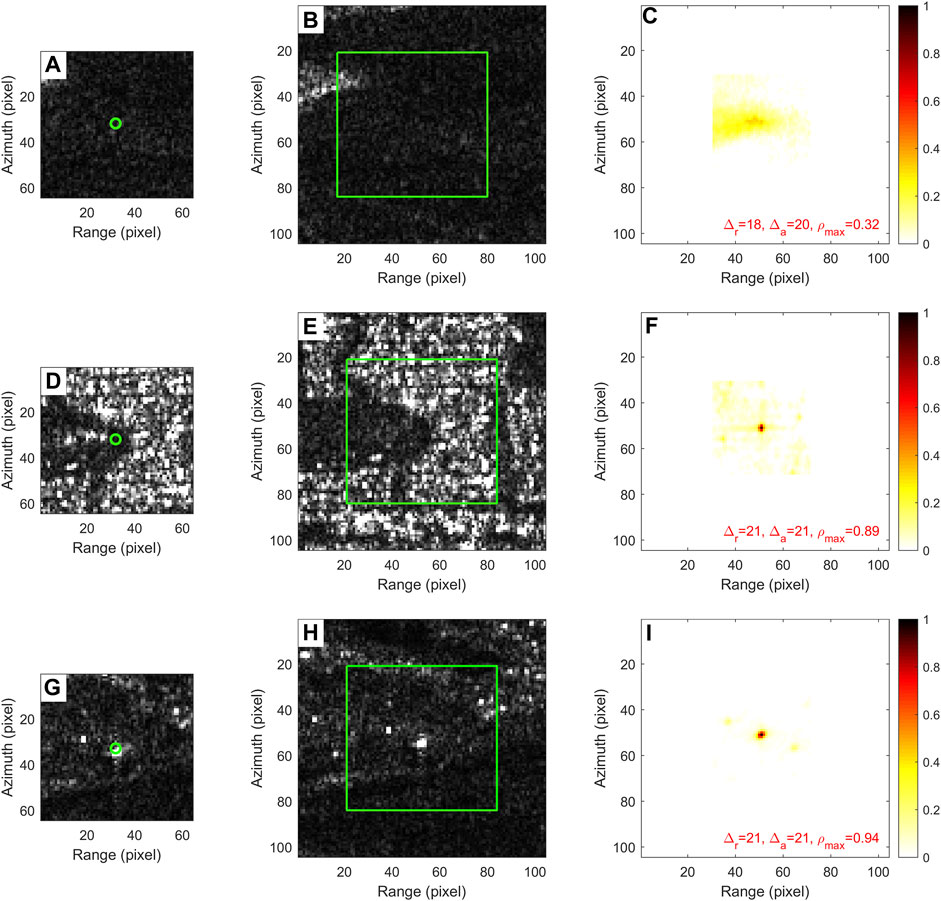
FIGURE 1. Cross-correlation of three tie points in radar amplitude images. (A) A blindly selected tie point in the green circle and its associated reference matching window. (B) The searching secondary window, in which the green box indicates the corresponding region with the same size of the reference window. (C) The coefficients from pixel-by-pixel cross-correlation, in which the red numbers denote range (${\Delta }_r$) and azimuth (${\Delta }_a$) offsets in pixels and the maximum coefficient (${\rho }_{\max }$). The corresponding figures for a dark and a bright feature point are shown in (D–F) and (G–I), respectively.

Speeded Up Robust Features (SURF) is one of the most popular methods for feature detection and description of remote sensing images (Bay et al., 2006). It has been used to match SAR images (Durgam et al., 2016; Liu and Wang, 2009). However, the registration accuracy using the SURF method is only at the level of ∼0.5 pixels (Durgam et al., 2016), which is much lower than the requirements of InSAR coregistration and offset tracking.

In this paper, we propose a feature point offset tracking (FPOT) procedure to improve the spatial resolution, reliability, and computing efficiency of the conventional method. The procedure consists of feature points detection with SURF, data masking with external land coverage data, cross-correlation analysis, quadtree filtering, and systematic offset removal. We conduct a real data analysis to assess the capability of RPOT by mapping co-seismic deformation associated with the 2016 Mw 7.8 Kaikōura earthquake using Sentinel-1 radar images.

Data

On November 14, 2016 (local time), the Mw 7.8 Kaikōura earthquake occurred in the northeastern part of the South Island of New Zealand (Figure 2). It is one of the largest earthquakes in New Zealand and one of the most complex earthquakes ever recorded on Earth (Hamling et al., 2017). The entire New Zealand reported a shock with widespread damage across much of the northern South Island. In the capital city, Wellington, at least two people were killed in the earthquake that occurred in the early hours of the day. SAR data showed that the earthquake triggered a significant partial rise in the northeastern part of the South Island, reaching a peak amplitude of about 8 m, with a horizontal displacement of more than 10 m in the active fault area, triggering a complex fault rupturing process (Hamling et al., 2017). Due to excessive deformation gradients, the near-field deformation of the earthquake cannot be correctly derived using the interferometric phase from the C-band Sentinel-1A data (Hamling et al., 2017).

FIGURE 2

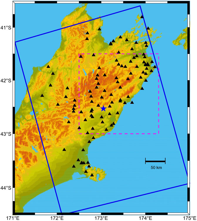
FIGURE 2. Color-shaded relief map of central New Zealand. The blue box indicates the coverage of the Sentinel-1A SAR imagery. The dashed magenta box shows the location of our study area for this study. The black triangles show GPS sites. The blue star in the middle denotes the epicenter of the Kaikōura earthquake.

Here, we apply our proposed FPOT approach on a pair of C-band Sentinel-1A ascending data collected on November 3, 2016 and November 15, 2016. The data were acquired in interferometric wide-swath mode (IW) on track 52, with pixel spacing of 2.3 by 14.1 m in slant range and azimuth directions, respectively. This corresponds to a spatial resolution of 5 by 20 m in ground range and azimuth directions, respectively (Torres et al., 2012; Yague-Martinez et al., 2016).

Materials and Methods

Figure 3 shows the flowchart of our FPOT procedure. First, the feature points in the reference single look complex (SLC) image are extracted using the SURF algorithm. Some unsatisfactory tie points are then discarded according to external land coverage data. The cross-correlation process is then applied to the remaining feature points. Outliers of offsets are removed using the adapted quadtree filtering. Finally, the resultant deformation field is derived after removing a bi-linear model fitted with far-field offsets.

FIGURE 3

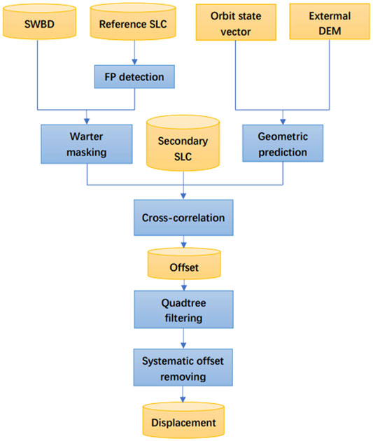
FIGURE 3. Flowchart of the FPOT procedure.

Feature Point Identification Using SURF

Bay et al. (2006) proposed the SURF algorithm to detect features based on Scale-Invariant Feature Transform (SHIF) (Lowe, 2004). SURF, a faster and more robust algorithm compared to the standard SHIF, is powerful to deal with a large volume of data, so that we can set relatively large matching windows to improve the reliability for feature points identification.

We use the SURF operator from the third-party open-source library OpenCV, an efficient tool for identifying feature points using SURF, to detect feature points (Bradski, 2000). To improve the speed in feature point identification and noise suppression, we convert the radar intensity with a range between the 2.5th and 97.5th percentile values of the cumulative image histograms to 0–255 scale. The pixels beyond the upper (97.5%) and lower (2.5%) bounds are set to 255 and 0, respectively. We set the window size to 24,000 × 6000 to speed up the calculation and prevent the entire detection window from lying in a water body. For large-scale images, we split the entire image into multiple blocks for parallel computing. By taking the advantage of OpenCV’s high computational efficiency, the processing time for the whole progress with 24,000 × 6000 pixels is only 167 s on a DELL laptop with AMD RYZEN 3600x CPU and 16G memory. Figure 4A shows the distribution of feature points with Hessian thresholds of 6000 and 10,000, respectively.

FIGURE 4

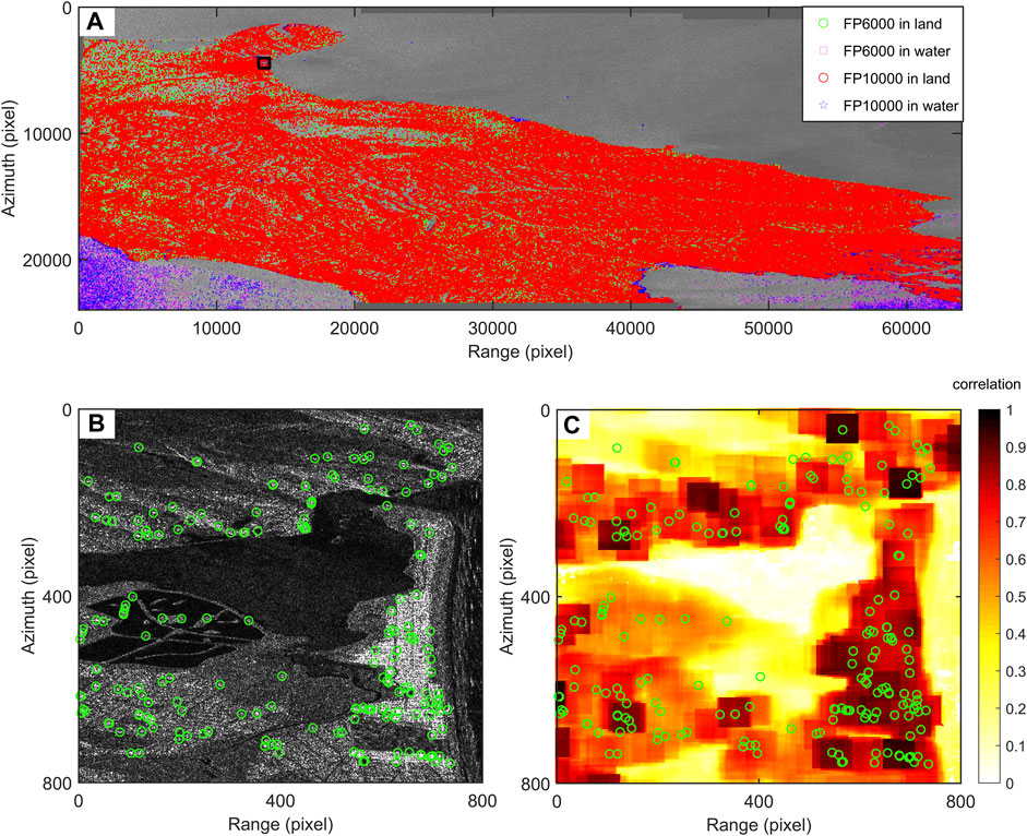
FIGURE 4. Distribution of feature points and cross-correlation degrees. (A) The green circles and the magenta squares represent feature points on land and in water, respectively, obtained by setting the Hessian threshold as 6000. The red circles and the blue stars are the corresponding feature points with the Hessian threshold of 10,000. (B) Zoom in of the area denoted as a black box in the upper-left corner in (A). Feature points are denoted as green circles. (C) Cross-correlation degrees of the amplitude image with a matching window size of 64 × 64 pixels and a step of 4 pixels. Pixels in water are not masked to show correlation comparison.

Feature Point Removal With Land Coverage Data

It is worth noting that some kinds of ground surface might not consist of proper feature points for offset tracking, for example, the water bodies in coastal areas, forests, deserts, and so on. Although SURF can somehow avoid selecting feature points in water bodies, some points still can be in the water for noisy amplitude images. The reasons include 1) the Hessian threshold is too low; 2) the search window is too small so that wrong feature points are selected due to random noise in the amplitude image; and 3) the entire search window is in the water. The correlation degrees of such feature points are expected to be low. It is a severe waste of time for matching these points because their resultant offsets are too noisy to be used for POT. Since many standard products are available already, e.g., the SRTM Water Body Data (SWBD) (NASA, 2013), we can mask the feature points lying in improper regions assisted with the land coverage information.

In the upper right corner of Figure 4A, a clear amplitude difference can be observed between water and land, and almost no feature points lie in the water. However, it can be seen from the bottom of Figure 4A that many feature points exist in the water, mainly because the coastal area comprises dense forests giving random noise in the amplitude image. In this situation, masking with water body data is necessary to remove these points. This can improve the efficiency and reliability of cross-correlation. Figure 4B is the zoom in of the region indicated using a black box in the upper-left corner of Figure 4A. The feature points, shown as green circles, are strongly related to the ground of corner points and urban buildings. These feature points have high degrees of correlation (Figure 4C) and rarely appear in low-correlation areas such as waters, farmlands, forests, etc.

Cross-Correlation and Quadtree Filtering

In cross-correlation, we set the reference and the search windows as 64 × 64 and 84 × 84 pixels, respectively, with an oversample factor of two and step size of 4 × 4 pixels. Figure 4C shows the cross-correlation degrees of all regular pixels in Figure 4B. The white holes indicate areas that are completely decorrelated and cannot be matched. It is obvious that most of the feature points are in high-correlation areas. For the whole image in Figure 4A, we use the cross-correlation approach on the remaining feature points and the resultant offsets are shown in Figure 5A.

FIGURE 5

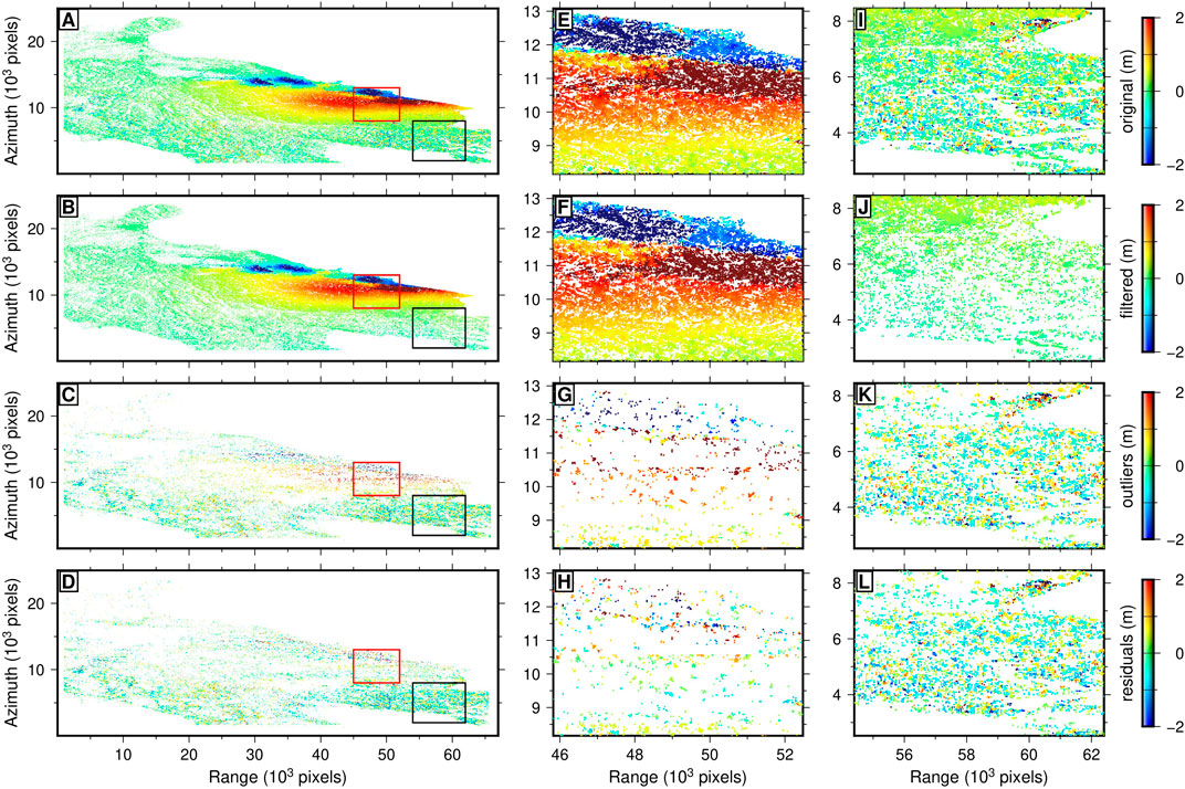
FIGURE 5. Quadtree filtering for range offsets. (A) Range offsets before and (B) after quadtree filtering. (C) Pixels removed by the filter. (D) Residuals between the observed offsets of the outliers and the mean of their associated quadrant. Red and black boxes in the first column correspond to near-field and far-field data, the corresponding figures are shown in (E–H) and (I–L), respectively.

The quadtree algorithm has been routinely used to reduce data points in high-resolution interferograms for geophysical modeling (Jónsson et al., 2002). Instead of using it for down-sampling, here we adapt the algorithm to remove outliers in the dataset as shown in Figure 5A. Our algorithm divides the whole image into quadrants, and then fit a bi-quadratic model of the offsets in each quadrant. If the RMSE in the quadrant exceeds a given threshold, the quadrant is further subdivided into four. Otherwise, we detect and remove the outliers based on a well-known robust scale estimator known as median absolute deviation (MAD). The bi-quadratic model is used because it can help keep the high deformation gradients. In addition, we subdivide the epicentral area into two regions with positive and negative values and apply filtering to them individually. These two strategies ensure that the pixels with the largest deformation are not removed. The adapted algorithm can well keep the major deformation features and remove noisy offsets, resulting in a high-resolution and reliable deformation field. Figure 5 shows a range of offsets before and after quadtree filtering. Figures 5E–L show a zoom in of quadtree filtering for the near-field and far-field areas denoted as red and black boxes in Figures 5A–D, respectively. We can see that most noisy pixels have been removed (Figures 5B,C). Figure 5D shows the residuals between the observed offsets of the outliers and the mean of their associated quadrant. The random signs of the residuals indicate that qualified data points are not culled out.

Systematic Offset Removal

The geometric offset of the orbits derives large-scale and systematic offsets between reference and secondary images. In conventional InSAR processing, coregistration is to constrain a transform matrix to convert a secondary image into a reference frame. The purpose of offset tracking is to measure offsets associated with deformation instead of orbit effects. Therefore, we first fit a bi-linear model using far-field offsets only, and then remove the predicted offsets to obtain the resultant deformation field. The bi-linear model is as

$\left[\begin{array}{c}{\mathrm{\Delta }}_r\\ {\mathrm{\Delta }}_a\end{array}\right]=\left[\begin{array}{c}{m}_1{m}_2\\ m_3{m}_4\end{array}\right]\left[\begin{array}{c}{r}_1\\ a_1\end{array}\right]+\left[\begin{array}{c}{m}_5\\ m_6\end{array}\right](1)$

where $m_1$ - $m_4$ are the rotation parameters, and $m_5$ - $m_6$ are the translation parameters, respectively. $r_1$ and $a_1$ are the range and the azimuth coordinates of the reference image, ${\mathrm{\Delta }}_r$ and ${\mathrm{\Delta }}_a$ are the range and the azimuth offsets of the secondary image relative to the reference image, respectively. The removal of such systematic offsets is the like InSAR coregistration, which we will discuss in Potentials for Applications in InSAR Coregistration.

Results and Discussion

Results

We apply the FPOT approach to derive the co-seismic deformation associated with the Kaikōura earthquake using the entire image shown in Figure 2. With a Hessian threshold of 6000 in the near-field and 10,000 in the far-field, we initially select 387,605 feature points from the reference image whose size is 24,302 $\times$ 66,213 pixels. For the RPOT approach, we select 390,602 regular points with steps of 64 and 32 pixels in range and azimuth directions, respectively. After the cross-correlation process, the outliers are culled out by a cross-correlation coefficient threshold of 0.45 and SNR threshold of 5. About 69% of the regular and 35% of the feature points are culled out. We then apply quadtree filtering, which removes 66,846 noisy points for the FPOT and 32,123 for the RPOT. Finally, we fit and remove the systematic offsets using far-field data points. The resultant points are 170,309 and 76,699 for the FPOT and RPOT, respectively. For a comparable number of preliminary points, the remaining qualified points for the FPOT approach are about twice the RPOT counterparts.

Figures 6A,B show the FPOT-derived range and azimuth offsets in the near field associated with the Kaikōura earthquake. Figures 6C,D show scatterplots of the displacements between FPOT-derived offsets (red), RPOT-derived offsets (blue), and GPS measurements projected to the range and azimuth directions, respectively. The results show good agreement between FPOT-derived range offsets and GPS measurements, with an RMSE of 14 cm. The RMSE of 48 cm in azimuth is higher than that of the range due to coarser azimuth resolution of the Sentinel-1A satellite. The RPOT-derived offsets have approximate agreements after culling out outliers, giving an RMSE of 15 and 55 cm for range and azimuth, respectively. Without removing the outliers, the RMSE of the RPOT-derived offsets are 37 and 69 cm in range and azimuth, respectively, which is larger than the corresponding values of 18 and 50 cm of the FPOT-derived offsets.

FIGURE 6

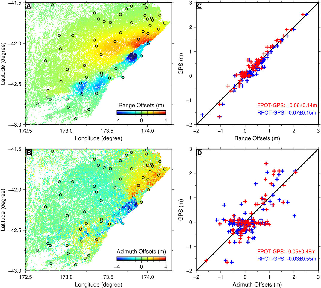
FIGURE 6. (A,B) FPOT-derived co-seismic displacements in range and azimuth directions, respectively. The black circles denote GPS sites color-coded with their displacements projected in range and azimuth directions. (C,D) Scatterplots show comparison between GPS displacements and FPOT-derived (red) and RPOT-derived (blue) offsets in range and azimuth. The corresponding FPOT value is the average offset within a 500 × 500 m box surrounding each GPS site.

Feature vs. Regular Points

Figures 7A,B are probability distribution of range and azimuth offsets of the entire SAR image after masking the near-field deformation. Therefore, the bias from 0 should be able to evaluate the accuracy of the algorithms. The histograms show that the RMSE of range offsets are reduced from 0.07 pixels for RPOT to 0.05 pixels for FPOT. This is further decreased to 0.03 pixels for FPOT after quadtree filtering. For azimuth offsets, the corresponding values decreased from 0.07 to 0.04 and 0.02 pixels, for RPOT, FPOT, and FPOT after quadtree filtering, respectively.

FIGURE 7

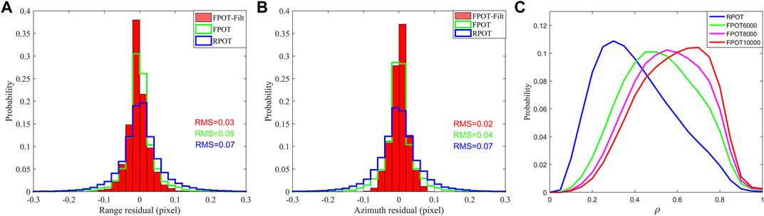
FIGURE 7. (A,B) Probability distribution of the range and azimuth offsets. One pixel spacing is 2.3 m in range and 14.1 m in azimuth. (C) Cross-correlation coefficients for regular and feature points.

The degree of cross-correlation is another important index for the quality of offset tracking. Figure 7C shows the probability distribution of the cross-correlation coefficients. The peak value of RPOT is ∼0.3, which is significantly lower than that of FPOT. With increasing Hessian threshold, we find that the number of feature points decreases (from 779,174 to 265,967) and the peak of cross-correlation coefficients increases (from 0.45 to 0.7).

Bright vs. Non-Bright Points

Bright points have often been used as tie points for offset tracking or coregistration (Serafino, 2006; Hu et al., 2014). However, some other points can also have apparent features, which can be considered as tie points in identifying offsets (Figure 1B). To test the degree to which bright and non-bright points contribute to offset tracking, we rescale the amplitudes of the identified feature points into the range between 0 and 255. Figure 8 shows the probability distribution of the grayscales with 10 levels. The brightest values between 230 and 255 account for ∼33% of the feature points, notably higher than any other level. The other levels have roughly uniform distribution at 6–10%, accounting for ∼67% in total. Although the brightest points account for the highest percentage, the non-bright points can significantly improve the number of feature points and the spatial resolution of the resultant deformation field.

FIGURE 8

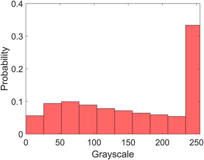
FIGURE 8. The grayscale histogram of all the feature points.

Potentials for Applications in InSAR Coregistration

Coregistration accuracy and efficiency are the two important factors for justifying the performance of the feature points for routine InSAR coregistration. At present, regular points are widely used in routine InSAR coregistration. Because regular points may be in a decorrelation area, many tie points are needed to ensure the accuracy and the reliability of affine matrix fitting. Our analysis above shows that feature points have high degrees of cross-correlation and reliable offset estimates. Therefore, a small number of feature points might satisfy the requirement for InSAR coregistration.

To test the feasibility of feature points for routine InSAR coregistration, we evaluate the accuracy of the coregistration affine matrix fitted using feature and regular points, respectively. We use a robust iterative least-square estimation. The outliers are identified and removed if the residuals are larger than 1.5 times of the posterior standard deviations. The inversion is converged when the RMSE is less than 0.08 pixels. We select 497 regular points with steps of 1024 pixels in the far field where co-seismic deformation is assumed to be negligible. To identify feature points, we set the detection window size as 6000 × 20,000 pixels and the Hessian threshold as 20,000. First, we select the same number of feature points as regular points to fit the affine matrix (Eq. 1). In the iteration inversion, the ratios of outliers are 83 and 27% for the regular and the feature points, respectively. The uncertainties of the resultant affine matrix fitted by feature points is about 1/3 of that fitted by regular points (Table 1). Second, we pick up the top 79 feature points with the largest response value in the detection window. We find that these points constrain the affine matrix even slightly better than that with 497 regular points. These two tests show that 1) the time-consuming cross-correlation operations for most regular points are not necessary in routine InSAR coregistration; and 2) only 1/6 of the size and computing time is required to achieve equal accuracy if the feature points are used instead of regular points.

TABLE 1

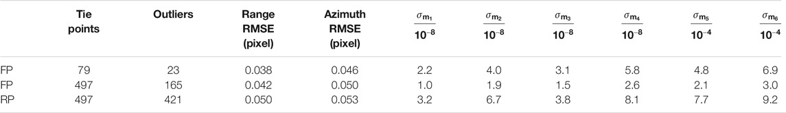
TABLE 1. The comparison of fitting affine matrix with feature and regular tie points.

Matching window size is another factor that affects the efficiency of InSAR coregistration. The smaller the search window size, the shorter the computing time. When the search window size is reduced in cross-correlation, nevertheless, the estimated offsets of some points might change much. Here we use the data in Figure 4B to test if feature points can reduce the matching window size while remaining reliable coregistration accuracy. To investigate the effect of matching window sizes to the matching success rate, we have conducted an experiment with reference matching window sizes from 64 × 64 to 8 × 8 pixels. Searching window sizes of 10 pixels larger than the corresponding reference matching windows are used in this experiment. For the case of FPOT, we find that the matching success rate has only dropped by 2% when comparing the reference window size of 64 × 64 pixels to 16 × 16 pixels. For the case of RPOT, a noticeable fall in matching success rates, by 13 and 36%, has been observed with the reference window size of 32 × 32 pixels and 16 × 16 pixels, respectively. Therefore, it is possible to use much smaller reference and search windows (i.e., 16 and 26 pixels, respectively) for FPOT while ensuring the offset’s reliability. These are much smaller than that of 64 and 84 pixels for the RPOT. This suggests that FPOT can further improve the coregistration efficiency.

Conclusions

The offset tracking method is an important complement to obtain large surface displacements in both azimuth and range directions where the InSAR technique is unfeasible due to excessive displacement gradients and phase unwrapping errors. To improve the reliability and efficiency of the standard method, we propose a method that combines SURF, external geographic data, cross-correlation, and quadtree filtering to derive reliable offset estimates. Application to the 2016 Mw 7.8 Kaikōura earthquake has shown that these feature points have distinct features that are helpful in identifying offsets. In offset tracking, feature points have higher amplitude cross-correlation than blindly selected regular points. In addition, feature points are not limited to bright points, and therefore have more observations, which can significantly improve the number of data points and the spatial resolution of the resulting deformation field. Furthermore, a smaller number of feature point matching patches can be used to achieve the equal coregistration accuracy of regular points, which can significantly improve the efficiency, accuracy, and reliability relative to standard coregistration. Considering the similarity of optical and SAR offset tracking, the procedure proposed in this study can also be used to improve deformation measurements in optical imagery (Avouac and Leprince, 2015; Leprince et al., 2007).

Data Availability Statement

The original contributions presented in the study are included in the article/Supplementary Material. Sentinel-1A images are provided freely by ESA's Sentinels Scientific Data Hub. SWBD are downloaded at http://geodata.policysupport.org/swbd. GPS data are from Hamling et al. (2017), which can be downloaded from http://www.sciencemag.org/cgi/content/full/science.aam7194/DC1. Further inquiries can be directed to the corresponding author.

Author Contributions

LP developed the cross-correlation algorithms, processed the data, and prepared a draft manuscript; HW designed the research and developed the quadtree filter; XY conducted quadtree filtering; LP, HW, AN and XY analyzed the data and wrote the paper.

Funding

This research is funded by the National Key Research and Development Program of China (2017YFC1500501), National Natural Science Foundation of China (41672205, 41774036), and the Program for Guangdong Introducing Innovative and Entrepreneurial Teams (2019ZT08L213).

Conflict of Interest

Author LP was employed by Urban and Rural Institute (Guangzhou) Co., Ltd.

The remaining authors declare that the research was conducted in the absence of any commercial or financial relationships that could be construed as a potential conflict of interest.

Publisher’s Note

All claims expressed in this article are solely those of the authors and do not necessarily represent those of their affiliated organizations, or those of the publisher, the editors, and the reviewers. Any product that may be evaluated in this article, or claim that may be made by its manufacturer, is not guaranteed or endorsed by the publisher.

References

Avouac, J. P., and Leprince, S. (2015). Geodetic Imaging Using Optical Systems. In: G. Schubert Editors Treatise on Geophysics (2nd Edition), 3, pp387-424, Oxford: Elsevier. doi:10.1016/b978-0-444-53802-4.00067-1

CrossRef Full Text | Google Scholar

Bay, H., Tuytelaars, T., and Van Gool, L. (2006). “SURF: Speeded Up Robust Features,” in Computer Vision - Eccv 2006 , Pt 1, Proceedings, Lecture Notes in Computer Science. 3951. Editors A. Leonardis, H. Bischof, and A. Pinz (Berlin: Springer-Verlag Berlin), 404–417. doi:10.1016/j.cviu.2007.09.01410.1007/11744023_32

CrossRef Full Text | Google Scholar

Bradski, G. (2000). The OpenCV Library. Dr. Dobb's J. Softw. Tools Pro Programmer 25 (11), 120–123.

Google Scholar

Durgam, U. K., Paul, S., and Pati, U. C. (2016). SURF based matching for SAR image registration, 2016 IEEE Students' Conference on Electrical, Electronics and Computer Science (SCEECS), 1-5. doi:10.1109/SCEECS.2016.7509292

CrossRef Full Text | Google Scholar

Elliott, J. R., Walters, R. J., and Wright, T. J. (2016). The Role of Space-Based Observation in Understanding and Responding to Active Tectonics and Earthquakes. Nat. Commun. 7, 16. doi:10.1038/ncomms13844

CrossRef Full Text | Google Scholar

Fialko, Y., Simons, M., and Agnew, D. (2001). The Complete (3-D) Surface Displacement Field in the Epicentral Area of the 1999 Mw 7.1 Hector Mine Earthquake, California, from Space Geodetic Observations. Geophys. Res. Lett. 28, 3063–3066. doi:10.1029/2001gl013174

CrossRef Full Text | Google Scholar

Goldstein, R. M., Zebker, H. A., and Werner, C. L. (2016). Satellite Radar Interferometry: Two-Dimensional Phase Unwrapping. Radio Sci. 23, 713–720.

Google Scholar

Hamling, I. J., Hreinsdóttir, S., Clark, K., Elliott, J., Liang, C., Fielding, E., et al. (2017). Complex Multifault Rupture during the 2016 Mw 7.8 Kaikōura Earthquake, New Zealand. Science 356 (6334), eaam7194. doi:10.1126/science.aam7194

PubMed Abstract | CrossRef Full Text | Google Scholar

Hooper, A., Bekaert, D., Spaans, K., and Arıkan, M. (2012). Recent Advances in SAR Interferometry Time Series Analysis for Measuring Crustal Deformation. Tectonophysics 514-517, 1–13. doi:10.1016/j.tecto.2011.10.013

CrossRef Full Text | Google Scholar

Hu, X., Wang, T., and Liao, M. (2014). Measuring Coseismic Displacements with Point-Like Targets Offset Tracking. IEEE Geosci. Remote Sensing Lett. 11, 283–287. doi:10.1109/lgrs.2013.2256104

CrossRef Full Text | Google Scholar

Jónsson, S., Zebker, H., Segall, P., and Amelung, F. (2002). Fault Slip Distribution of the 1999 Mw 7.1 Hector Mine, California, Earthquake, Estimated from Satellite Radar and GPS Measurements. Bull. Seismological Soc. America 92, 1377–1389. doi:10.1785/0120000922

CrossRef Full Text | Google Scholar

Lasserre, C., Peltzer, G., Crampé, F., Klinger, Y., Van der Woerd, J., and Tapponnier, P. (2005). Coseismic Deformation of the 2001 Mw = 7.8 Kokoxili Earthquake in Tibet, Measured by Synthetic Aperture Radar Interferometry. J. Geophys. Res. 110, 22. doi:10.1029/2004jb003500

CrossRef Full Text | Google Scholar

Leprince, S., Barbot, S., Ayoub, F., and Avouac, J.-P. (2007). Automatic and Precise Orthorectification, Coregistration, and Subpixel Correlation of Satellite Images, Application to Ground Deformation Measurements. IEEE Trans. Geosci. Remote Sensing 45, 1529–1558. doi:10.1109/TGRS.2006.888937

CrossRef Full Text | Google Scholar

Liu, R., and Wang, Y. (2007). SAR Image Matching base on Speeded Up Robust Feature. IEEE Int. Conf. on Intell. Syst. 4, 518–522. doi:10.1109/GCIS.2009.297

CrossRef Full Text | Google Scholar

Lowe, D. G. (2004). Distinctive Image Features from Scale-Invariant Keypoints. Int. J. Comp. Vis. 60, 91–110. doi:10.1023/b:Visi.0000029664.99615.94

CrossRef Full Text | Google Scholar

Massonnet, D., and Feigl, K. L. (1998). Radar Interferometry and its Application to Changes in the Earth's Surface. Rev. Geophys. 36, 441–500. doi:10.1029/97rg03139

CrossRef Full Text | Google Scholar

Michel, R., Avouac, J. P., and Taboury, J. (1999). Measuring Ground Displacements from SAR Amplitude Images: Application to the Landers Earthquake. Geophys. Res. Lett. 26, 875–878. doi:10.1029/1999gl900138

CrossRef Full Text | Google Scholar

NASA JPL. (2013). NASA Shuttle Radar Topography Mission Water Body Data Shapefiles & Raster Files [Data set]. NASA EOSDIS Land Processes DAAC. Accessed 2021--12-06. Available at: http://wMEaSUREs/SRTM/SRTMSWBD.003.

Google Scholar

Ng, A. H. M., Ge, L., Du, Z., Wang, S., and Ma, C. (2017). Satellite Radar Interferometry for Monitoring Subsidence Induced by Longwall Mining Activity Using Radarsat-2, Sentinel-1 and ALOS-2 Data. Int. J. Appl. Earth Observation Geoinformation 61, 92–103. doi:10.1016/j.jag.2017.05.009

CrossRef Full Text | Google Scholar

Pagli, C., Sigmundsson, F., Pedersen, R., Einarsson, P., Arnadóttir, T., and Feigl, K. L. (2007). Crustal Deformation Associated with the 1996 Gjálp Subglacial Eruption, Iceland: InSAR Studies in Affected Areas Adjacent to the Vatnajökull Ice Cap. Earth Planet. Sci. Lett. 259, 0–33. doi:10.1016/j.epsl.2007.04.019

CrossRef Full Text | Google Scholar

Serafino, F. (2006). SAR Image Coregistration Based on Isolated Point Scatterers. IEEE Geosci. Remote Sensing Lett. 3, 354–358. doi:10.1109/lgrs.2006.872399

CrossRef Full Text | Google Scholar

Sturkell, E., Einarsson, P., Sigmundsson, F., Geirsson, H., Ólafsson, H., Pedersen, R., et al. (2006). Volcano Geodesy and Magma Dynamics in Iceland. J. Volcanology Geothermal Res. 150, 14–34. doi:10.1016/j.jvolgeores.2005.07.010

CrossRef Full Text | Google Scholar

Torres, R., Snoeij, P., Geudtner, D., Bibby, D., Davidson, M., Attema, E., et al. (2012). GMES Sentinel-1 Mission. Remote Sensing Environ. 120, 9–24. doi:10.1016/j.rse.2011.05.028

CrossRef Full Text | Google Scholar

Wang, H., Elliott, J. R., Craig, T. J., Wright, T. J., Liu-Zeng, J., and Hooper, A. (2014). Normal Faulting Sequence in the Pumqu-Xainza Rift Constrained by InSAR and Teleseismic Body-Wave Seismology. Geochem. Geophys. Geosyst. 15, 2947–2963. doi:10.1002/2014gc005369

CrossRef Full Text | Google Scholar

Wang, H., Ge, L., Xu, C., and Du, Z. (2007a). 3-D Coseismic Displacement Field of the 2005 Kashmir Earthquake Inferred from Satellite Radar Imagery. Earth Planet. Sp 59, 343–349. doi:10.1186/bf03352694

CrossRef Full Text | Google Scholar

Wang, H., Wright, T. J., Liu‐Zeng, J., and Peng, L. (2019). Strain Rate Distribution in South‐Central Tibet from Two Decades of InSAR and GPS. Geophys. Res. Lett. 46, 5170–5179. doi:10.1029/2019gl081916

CrossRef Full Text | Google Scholar

Wang, H., Xu, C., and Ge, L. (2007b). Coseismic Deformation and Slip Distribution of the 1997 7.5 Manyi, Tibet, Earthquake from InSAR Measurements. J. Geodynamics 44, 200–212. doi:10.1016/j.jog.2007.03.003

CrossRef Full Text | Google Scholar

Wang, T., and Jonsson, S. (2015). Improved SAR Amplitude Image Offset Measurements for Deriving Three-Dimensional Coseismic Displacements. IEEE J. Sel. Top. Appl. Earth Observations Remote Sensing 8, 3271–3278. doi:10.1109/jstars.2014.2387865

CrossRef Full Text | Google Scholar

Wang, T., Wei, S., Shi, X., Qiu, Q., Li, L., Peng, D., et al. (2018). The 2016 Kaikōura Earthquake: Simultaneous Rupture of the Subduction Interface and Overlying Faults. Earth Planet. Sci. Lett. 482, 44–51. doi:10.1016/j.epsl.2017.10.056

CrossRef Full Text | Google Scholar

Wright, T. J., Ebinger, C., Biggs, J., Ayele, A., Yirgu, G., Keir, D., et al. (2006). Magma-maintained Rift Segmentation at Continental Rupture in the 2005 Afar Dyking Episode. Nature 442, 291–294. doi:10.1038/nature04978

PubMed Abstract | CrossRef Full Text | Google Scholar

Wright, T. J., Elliott, J. R., Wang, H., and Ryder, I. (2013). Earthquake Cycle Deformation and the Moho: Implications for the Rheology of Continental Lithosphere. Tectonophysics 609, 504–523. doi:10.1016/j.tecto.2013.07.029

CrossRef Full Text | Google Scholar

Yague-Martinez, N., Prats-Iraola, P., Rodriguez Gonzalez, F., Brcic, R., Shau, R., Geudtner, D., et al. (2016). Interferometric Processing of Sentinel-1 TOPS Data. IEEE Trans. Geosci. Remote Sensing 54, 2220–2234. doi:10.1109/TGRS.2015.2497902

CrossRef Full Text | Google Scholar

Zebker, H. A., and Chen, K. (2005). Accurate Estimation of Correlation in InSAR Observations. IEEE Geosci. Remote Sensing Lett. 2, 124–127. doi:10.1109/lgrs.2004.842375

CrossRef Full Text | Google Scholar