Dissecting a Zombie: Joint Analysis of Density and Resistivity Models Reveals Shallow Structure and Possible Sulfide Deposition at Uturuncu Volcano, Bolivia

1 Introduction

The identification of unrest at several Pleistocene age volcanoes, sometimes described as “zombie” volcanoes (Pritchard et al., 2014), has interesting implications for both hazard assessment and interpretation of extinct volcanic systems preserved in the geologic record. While some of these systems may simply have very long repose times (Taapaca Volcanic Complex, Chile; Clavero et al., 2004), in some cases the observed unrest may be driven by mechanisms that do not necessarily indicate impending eruption, particularly hydrothermal processes (Fournier and Chardot, 2012). These zombie systems complicate a common definition of an “active” or “dormant” volcano as a volcano that has erupted in historical times or the last 10 kyr, introducing a grey area between “dormant” and “extinct”. While observations of currently or recently eruptive systems are plentiful, the surface activity and subsurface processes (or lack thereof) we would expect at an extinct or near-extinct volcanic system are less clear. In addition to raising critical questions related to assessing volcanic hazard (how do we distinguish an active volcano with long repose intervals from benign processes occurring at an extinct system?), observations of these “zombie” systems have the potential to link processes inferred from the geologic record (formation of ore deposits) to processes we can observe in the present day. A key goal of this paper is to better understand possible causes of activity at zombie volcanoes, including rejuvenation of the magmatic system leading to an eruption, movement of hydrothermal fluids, and potentially even processes related to ore formation.

The connection between magmatic processes and a large percentage of the world’s economically viable ore deposits is well-established in the literature (Hedenquist and Lowenstern, 1994; Sillitoe, 2010). For example, copper-porphyry deposits are thought to form in an altered pluton (Sillitoe, 2010), while significant gold deposits likely form in the shallower hydrothermal system above a degassing magma body (Hedenquist and Lowenstern, 1994). In general, saline hydrothermal fluids of either magmatic or meteoric origin are considered critical for transporting and concentrating economic quantities of metallic elements, which have the potential to form an ore body if trapped and allowed to accumulate in the subsurface (Hedenquist and Lowenstern, 1994; Sillitoe, 2010; Blundy et al., 2015). Magnetotelluric imaging has identified zones of low resistivity (<1 Ω m) beneath several volcanoes worldwide (Aizawa et al., 2005; Yamaya et al., 2013) that may represent accumulations of saline fluids. Modeling by Afanasyev et al. (2018) showed that these brine lenses may be quite long lived, persisting more than 250 kyr after the cessation of active degassing from a source magma body. Analysis of injection-induced swarm seismicity by Cox (2016) suggests that hydrothermal ore deposits are likely formed from short-lived, transient pulses of super critical fluids with recurrence intervals of years to decades, rather than a slow, gradual process. Blundy et al. (2015) suggest that copper porphyry deposits may be formed via two pulses of fluids—first, a pulse of brine rich fluids that persists in the subsurface, followed by a gas-rich pulse that triggers deposition of ore-bearing sulfides.

Uturuncu, a “zombie” volcano located in the southwestern corner of Bolivia (Figure 1), has been the focus of an interdisciplinary research effort (Pritchard et al., 2018) aimed in part at understanding the source of a globally anomalous (Ebmeier et al., 2018), 140 km wide pattern of uplift surrounded by a subsidence moat (Figure 1, Pritchard and Simons, 2004; Fialko and Pearse, 2012; Henderson and Pritchard, 2013; Lau et al., 2018; Eiden et al., 2020), at a volcano whose last known eruption was 250 kyr ago (Muir et al., 2015). Analysis of decades of InSAR, GPS, and leveling data determined that the rate of uplift is variable on a decadal scale (Henderson and Pritchard, 2017), and has been ongoing for at least the past 50 years (Gottsmann et al., 2018). Geomorphological evidence suggests that the current deformation episode is transient, having lasted no longer than about 100 years (Perkins et al., 2016). More recent InSAR observations also show a small zone of subsidence to the south of Uturuncu that began after 2014 and continued until 2017 (Lau et al., 2018; Eiden et al., 2020). Pritchard et al. (2018) presented a synthesis of available data at Uturuncu and concluded that the deformation at Uturuncu is best explained by transient migration and shallow (<10 km depth) entrapment of volatiles and aqueous fluids originating from the Altiplano-Puna Magma/Mush Body (APMB), a large mid-crustal zone of partial melt (Ward et al., 2014; McFarlin et al., 2018). Numerical modeling by Gottsmann et al. (2017) shows that the deformation signal can be reproduced by pressurization of either a magmatic (top at −6 km above sea level (a.s.l.)) or hybrid dacite/fluid (top at sea level) column and basal bulge extending from the APMB, with simultaneous radial depressurization of the APMB. (In order to have a consistent frame of reference, all depths and elevations will be reported in km above sea level (a.s.l.). Locations below sea level, e.g., 10 km below sea level, will be negative in this system, e.g., −10 km a.s.l. For reference, the average elevation in the study area is 4.5 km a.sl., and the summit of Uturuncu is 6 km a.s.l.).

FIGURE 1

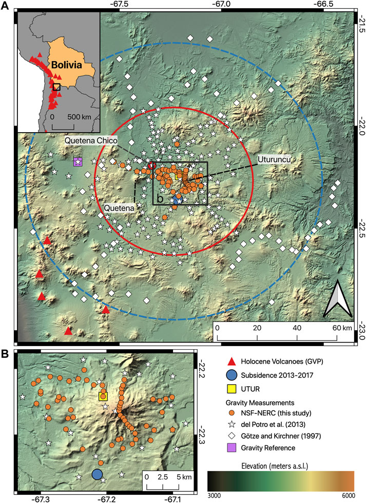
FIGURE 1. Overview map of Uturuncu and surroundings with inset map showing the study area relative to Bolivia and South America. The gravity measurements from 2018 are marked with orange circles. Measurement locations from older surveys are marked with white symbols, and the gravity reference is marked by a purple square. The large red and blue circles denote the areas of approximately radial uplift and subsidence, respectively, (Pritchard and Simons, 2004; Fialko and Pearse, 2012; Henderson and Pritchard, 2013). The small solid blue circle marks the subsidence area south of Uturuncu identified by Lau et al. (2018) and Eiden et al. (2020). The black rectangle in (A) shows the extent of the map in (B) that highlights the locations of the 2018 measurements on the edifice of Uturuncu. Digital elevation map (DEM) from (NASA/METI/AIST/Japan Spacesystems and U.S./Japan ASTER Science Team, 2019). The red stars are the locations of Holocene volcanoes (Global Volcanism Program, 2013) and the yellow square is the continuous GNSS station UTUR (Henderson and Pritchard, 2017).

Critically, the available evidence is not consistent with melt accumulation at depths shallower than −4 km a.s.l. Pritchard et al. (2018) argue that Uturuncu most likely represents a waning volcanic system. While magnteotelluric data did identify a <1 Ω m resistivity anomaly at sea level, because dacite melt is relatively resistive (5 Ω m), Comeau et al. (2016) determine that saline fluids better explained the low resistivity. This zone may instead represent an active hydrothermal system hosting 30,000 ppm salinity fluid (Pritchard et al., 2018). Calculations of regional seismic b-values using moment magnitudes are consistent with swarm seismicity, providing further evidence for active fluid transfer in this area (Hudson et al., 2021). The combination of transient deformation in a waning magmatic system with the presence of saline fluids make the upper 10 km of the crust at Uturuncu a key target for understanding possible mechanisms of unrest in a post-eruptive volcanic system and, potentially, the early stages of ore body formation (Sillitoe, 2010; Blundy et al., 2015; Cox, 2016).

Key to understanding the processes occurring beneath Uturuncu is mapping the density variations constrained by measurements of spatial gravity changes. While gravity modeling is mathematically non-unique (LaFehr and Nabighian, 2012), at Uturuncu we have a wealth of geophysical (Jay et al., 2012; Ward et al., 2014; Comeau et al., 2016; Kukarina et al., 2017; Hudson et al., 2021) and petrological (Sparks et al., 2008; Muir et al., 2014b; Muir et al., 2014a; Muir et al., 2015) information to constrain our modeling. When used in conjunction with other data sets, gravity measurements can be a powerful tool for understanding complex volcanic structures (Trevino et al., 2021), highlighting features other methods may be blind to. A density model of the upper 10 km at Uturuncu of comparable resolution to the existing resistivity model could falsify or support the presence of saline fluids at Uturuncu and their contribution to the deformation signal. Additional detailed density information may also establish to what degree Uturuncu could serve as a modern-day analogue for hydrothermal ore deposits (Blundy et al., 2015).

Any interpretation derived from a single geophysical property is inherently ambiguous. The shallow low resistivity anomaly at Uturuncu is consistent with at least three scenarios: saline fluids, high dacite melt fractions, or even high concentrations of conductive metallic deposits (Comeau et al., 2016; Pritchard et al., 2018). While some scenarios are considerably less likely, they cannot be ruled out on the basis of resistivity alone. However, these three scenarios would have quite different densities, with the potential to falsify any one of these hypotheses. Gravity surveys have imaged subsurface density structure at multiple volcanic systems (Zurek and Williams-Jones, 2013; Young et al., 2020; Trevino et al., 2021). A gravity inversion by del Potro et al. (2013) revealed a ca 15 km wide low density column rising from the APMB beneath Uturuncu, but this model lacks sufficient resolution to compare with the low resistivity anomalies Comeau et al. (2016) imaged in the upper 10 km.

This paper presents new gravity data collected in November 2018 on the edifice of Uturuncu in order to investigate the density structure of the upper 10 km of the crust, combined with existing regional gravity data from Götze and Kirchner (1997) and del Potro et al. (2013). We present an updated Bouguer anomaly map of Uturuncu and analysis of this map, comprising derivative analysis and a full 3-D inversion. We then analyze the recovered density model in tandem with the resistivity model of Comeau et al. (2016) and other available petrological and geophysical information. Finally, we conclude that the shallow density and resistivity anomalies at Uturuncu are consistent with the presence of saline fluids, revealing a complex zone of fracturing and hydrothermal alteration surrounding a shallow zone of potential sulfide deposition.

2 Geologic Setting and Previous Work

Uturuncu volcano is part of the Central Andean Volcanic Zone caused by the subduction of the Nazca plate under the South American plate (Barazangi and Isacks, 1976). Uturuncu itself is behind the main arc, surrounded by the Altiplano-Puna Volcanic Complex (de Silva, 1989), which overlies the APMB in the mid-crust (Ward et al., 2014; McFarlin et al., 2018). The Altiplano-Puna Volcanic Complex (APVC) erupted a cumulative volume of >15,000 km³ of ignimbrites between 11 and 1 Ma (de Silva, 1989), following a steepening of the subducting slab at 16 Ma from nearly flat-slab suduction to today’s 30° dip angle (Barazangi and Isacks, 1976; Allmendinger et al., 1997). Multiple authors argue that the change in subduction angle led to decompression and dehydration melting in the overlying mantle wedge and delamination of the base of the continental lithosphere (Allmendinger et al., 1997; Kay and Coira, 2009). Crustal thickness in this region can reach 60–70 km (Prezzi et al., 2009).

Uturuncu and the APVC overlie the Altiplano-Puna Magma Body (APMB), a large zone of mid-crustal partial melt extending from −4 to −25 km a.s.l. (Ward et al., 2014; McFarlin et al., 2018). Joint interpretation of the resistivity model derived from magnetotelluric measurements (Comeau et al., 2016) and seismic velocity models derived from receiver functions and earthquake and ambient noise tomography suggest that the APMB is compositionally zoned, with partially molten dacite from −4 to −13 km a.s.l. overlying partially molten andesite from −13 to −25 km a.s.l. (Jay et al., 2012; Ward et al., 2014; Kukarina et al., 2017; McFarlin et al., 2018; Pritchard et al., 2018).

Geological maps of the region surrounding Uturuncu have limited information about bedrock geology and structure due to the thick ignimbrite cover of the APVC (Servicio Geológico de Bolivia, 1968, 1973; Pareja and Ballón, 1978). In spite of the violent context of the APVC (de Silva, 1989; Salisbury et al., 2011), known eruptive products from Uturuncu consist entirely of effusive dacitic lava flows (Sparks et al., 2008; Muir et al., 2014a). Melt inclusion entrapment pressures from the 250 kyr dacites point to a storage depth of sea level to 2 km a.s.l., ruling out pre-eruptive emplacement of dacite magma at Uturuncu as the source of the 140 km deformation signal (Muir et al., 2014a; Pritchard et al., 2018), as such a wide signal points to a much deeper deformation source than 0–2 km a.s.l. (Pritchard and Simons, 2004; Fialko and Pearse, 2012; Henderson and Pritchard, 2017). Gravity forward modeling (Prezzi et al., 2009) and comparisions of compositional data from exposed basement rocks with geophysical data (Lucassen et al., 2001) suggest that upper-crustal basement rocks in the region most likely consist of gneisses with a felsic composition.

Regional tectonics around Uturuncu reflect a shift from compression to gravitational collapse tied to the change in slab steepness (Riller et al., 2001; Giambiagi et al., 2016). NW trending strike-slip fault systems dominate, with minor normal faulting (Cladouhos et al., 1994). Sparks et al. (2008) identified a NW trending fault off Uturuncu’s western flank, and Gioncada et al. (2010) identified NW lineaments near Uturuncu. Seismic anisotropy measurements by Maher and Kendall (2018) show a complex local pattern of fast shear-wave polarization direction at Uturuncu overprinting a regional pattern of EW stress. A radial pattern of fast shear-wave polarization dominates on Uturuncu’s western flank, with NW deflections of the regional stress occurring to the NW and SE of the edifice, possibly related to the NW trending fault identified by Sparks et al. (2008). Topographic analysis of local lineaments by Walter and Motagh (2014) similarly identified a girdle of fractures and lineaments surrounding Uturuncu.

3 Data and Methods

3.1 Gravity Data and Reduction

The 282 gravity measurements used in this analysis consist of three distinct data sets collected at different times: gravity measurements originally published in del Potro et al. (2013) and Götze and Kirchner (1997), as well as more recent measurements collected in October and November of 2018 (Figure 1). The details of these data sets are summarized in Tables 1, 2.

TABLE 1

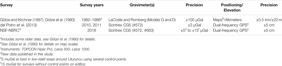
TABLE 1. Survey information for gravity data.

TABLE 2

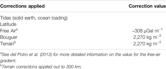
TABLE 2. Gravity data reductions.

Data collected in October and November of 2018 consisted of re-occupations of pre-existing microgravity measurement sites and 46 new measurements along several profiles primarily on the Uturuncu edifice, with station spacings ranging from 100 s of meters up to 2 km. New static gravity data were collected using a Scintrex CG-5 Autograv gravimeter (serial number: 572) in unison with a TOPCON HiPer Pro Dual-Frequency Global Navigation Satellite System (GNSS) base and rover system. The precision of repeat measurement was ±15 μGal (average of five cycles of 45 s long readings of 6 Hz raw data at each benchmark). GNSS data were recorded for 10–15 min at 1 Hz at the survey benchmarks using a roving receiver/antenna unit. The base receiver/antenna unit located at Quetena Chico (Figure 1) recorded continuously at 1 Hz during the survey period. The derived precision of the benchmark locations was <0.1 m in the vertical and <0.07 m in the horizontal after baseline processing of the benchmark locations against the base station, a cGPS station operating near the summit of Uturuncu (UTUR, Figure 1) and up to 15 regional reference stations using the AUSPOS online processing service.

Using the same methods as in del Potro et al. (2013) we tied the gravity datasets together by finding a best-fit offset value that minimized the difference in Bouguer gravity values between the datasets at select areas where measurement locations overlapped between surveys (see del Potro et al. (2013) for more details). We then applied the gravity corrections outlined in Table 2 and described below to isolate the Bouguer anomaly, which included solid Earth tides, latitude, free air, Bouguer, and terrain corrections. For all subsequent analysis we used only the Bouguer anomaly map, as the Bouguer anomaly should show gravity variations due only to changes in subsurface density.

We reduced the raw gravity data for tidal effects using the Wahr-Dehant (Dehant et al., 1999) and GOT99.2 (Ray, 1999) latitude-dependent models for solid Earth tides and ocean tides, respectively. For the terrain correction we used the 90 m Shuttle Radar Topography Mission (Farr et al., 2007) data to construct an initial digital elevation model (DEM) of the area up to 300 km from Uturuncu. Using ellipsoidal heights from 282 gravity benchmarks occupied during earlier surveys and the current, we corrected for offsets in the elevation data between the DEM and the GNSS data. This permitted us to correct the gravity data for terrain effects using an automated routine based on the approach of Hammer (1939). However, we calculated the terrain correction at each DEM data point rather than for each Hammer chart compartment. After calculating the distances Δd between a benchmark and all data points of the gridded DEM via

$\mathrm{\Delta }d=\left(\frac{1}{r}-\frac{1}{(r^2+\mathrm{\Delta }{z}^2)}\right)\mathrm{\Delta }{x}^2(1)$

the total terrain correction (TC) for each benchmark can be calculated via

$TC=\rho G\sum \mathrm{\Delta }d(2)$

where r is the radial distance from the benchmark to each DEM data point in metres, Δz is the elevation difference between the benchmark and the DEM data point, Δx is the DEM spacing. G is the universal gravitational constant and ρ is the terrain density. Locations of gravity benchmarks were selected as to minimize effects of the near-field terrain (up to 180 m distance from each measurement point). We therefore avoided taking measurements near abrupt topographic changes such as ridges or valleys.

3.2 Methods

A key goal in this study was to constrain the shallow density structure at Uturuncu, which we approached by analyzing the gravity data with both derivative analysis and geophysical inversion. Derivative analysis of the Bouguer gravity anomaly map preferentially highlights shallow density structures at the depths of interest, while geophysical inversion produces a 3-D density model that can be directly compared with the resistivity model of Comeau et al. (2016). Additionally, these two complementary techniques provide two independent analyses of the same data set for cross-checking the results.

3.2.1 Derivative Analysis

To delineate shallow structures at Uturuncu we performed several types of derivative analysis on the interpolated Bouguer anomaly map. The first and second spatial derivatives emphasize changes in the Bouguer anomaly, and act as a high pass filter, emphasizing short wavelength features caused by shallow features or abrupt density changes, such as faults (Gudmundsson and Högnadóttir, 2007). We first interpolated the gravity data points using a multiquadrics radial basis function algorithm (Chirokov, 2020), including an optional smoothing parameter to reduce the effect of outlier data points on the map. Our derivative analysis included the following calculations, displayed in Eqs 3–6, in which g is the Bouguer anomaly; the second vertical derivative is SVD (Eq. 3, LaFehr and Nabighian, 2012), the total horizontal gradient is THDR (Eq. 4, Cordell, 1979), the analytic signal is AS (Eq. 5, Nabighian, 1972), and the tilt angle is TA (Eq. 6, Miller and Singh, 1994).

$SVD=-\left(\frac{{\partial }^{2}g}{\partial x^2}+\frac{{\partial }^{2}g}{\partial y^2}\right)(3)$

$THDR=\sqrt{{\left(\frac{\partial g}{\partial x}\right)}^2+{\left(\frac{\partial g}{\partial y}\right)}^2}(4)$

$\left|AS\right|=\sqrt{{\left(\frac{\partial g}{\partial x}\right)}^2+{\left(\frac{\partial g}{\partial y}\right)}^2+{\left(\frac{\partial g}{\partial z}\right)}^2}(5)$

$TA={\tan }^{-1}\left(\frac{\partial g/\partial z}{THDR}\right)(6)$

3.2.2 Inversion

Using the gravity data described above, we solved for a suite of possible density models using the inversion algorithm GROWTH2.0 (Camacho et al., 2011). GROWTH2.0 solves for a density model via a non-linear inversion algorithm in which the algorithm “grows” anomalous bodies of user-defined maximum density contrast bounds from randomly distributed seeds based on a balance between fit to data and model smoothness. The primary inversion parameters to explore are the density contrast bounds and the balance factor that controls the weighting between fit to data and model smoothness. The user can also specify a linear or exponential background density contrast increase and a “homogeneity” factor that controls the sharpness of the density anomaly boundaries in the model. The inversion algorithm also automatically solves for and removes a bilinear regional trend.

For our inversion we used a subset of 215 of the gravity measurements mapped in Figure 1 (See the Data Availability Statement for how to access a complete table of gravity measurements). We excluded more distal measurements to focus the inversion on the shallow structure beneath Uturuncu. We also removed 4 measurements with high inversion residuals in preliminary inversion runs. Two of these points were measurements from the lower-precision Götze and Kirchner (1997) survey co-located with measurements from the higher-precision del Potro et al. (2013) survey (Table 1), and two of these points were microgravity stations in areas of high topographic relief where properly accounting for the terrain effect is difficult.

We followed the recommended procedures in Camacho et al. (2007) to choose appropriate balance factors and a range of density contrasts. First we explored for an appropriate range of density contrast bounds by keeping the balance factor constant and noting when anomalies started to become either “skeletal” (Figure 2A) or “inflated” (Figures 2B,C). In skeletal models a significant portion of the anomalies will start to disappear, in which parts of larger anomalies will become disconnected and smaller anomalies disappear altogether (Figure 2A). In inflated models anomalies will appear saturated and new fictitious anomalies will appear in some areas (Figure 2C). We found that positive density contrast bounds between +120 and +250 kg m⁻³ and negative density contrast bounds between −180 and −120 kg m⁻³ worked well, producing models that were neither skeletal nor inflated. We then chose balance factors for models with ±120, ±150, and −180/+250 kg m⁻³ density contrast bounds such that the first autocorrelation point is at zero, as described in (Camacho et al., 2007). Our final suite of models all have autocorrelation values of 0.02 or less, and between 1.1 and 1.3 mGal standard deviation in the residuals, comparable to the previously published inversion by del Potro et al. (2013), but with considerably improved shallow resolution. The low autocorrelation value indicates that our models adequately fit signals present in the data without over-fitting fictitious features to noise in the data.

FIGURE 2

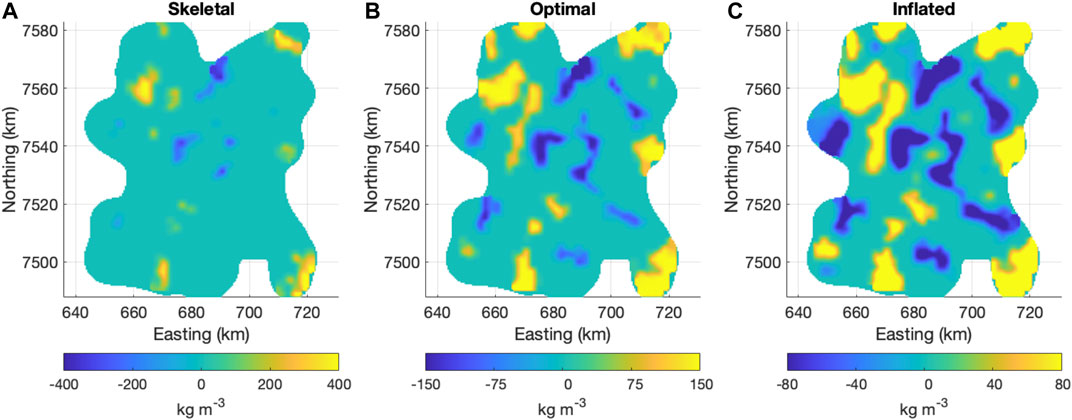
FIGURE 2. Depth slices at sea level of skeletal, optimal, and inflated density models produced with GROWTH2.0. (A) Skeletal model produced with too large density contrast bounds (±400 kg m⁻³). (B) Optimal model produced with ±150 kg m⁻³ density contrast bounds (C) Inflated model produced with too small density contrast bounds (±80 kg m⁻³).

The user-specified homogeneity factor in GROWTH2.0 can range from 0 to 1, where higher values lead to smoother anomaly edges. We explored a range of homogeneity values, and found that changing the homogeneity value did not significantly alter the dimensions and locations of the primary features of the model. However, higher homogeneity values introduced more noisy features to the model, so we opted for the lower value of 0.2.

4 Results and Verification

4.1 Bouguer Gravity Anomaly

Figure 3 displays the interpolated Bouguer anomaly map. In agreement with Götze and Kirchner (1997); Prezzi et al. (2009); del Potro et al. (2013), we also find a negative Bouguer anomaly centered on Uturuncu (Figure 3). Additionally, our survey reveals an elongated positive gravity anomaly to the northwest of Uturuncu, and two negative gravity anomalies to the southeast of Uturuncu (Figure 3).

FIGURE 3

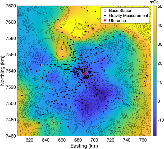
FIGURE 3. Map of interpolated Bouguer gravity anomaly (fill color) overlain by topography (black lines) from the 90 m SRTM DEM (Farr et al., 2007). Black dots are gravity measurement locations, white square is reference station, red triangle is location of Uturuncu.

4.2 Derivative Analysis

Figure 4 shows the four kinds of derivative analysis described in Section 3.2.1 applied to the Bouguer gravity anomaly at Uturuncu. Several features are prominent in all four kinds of derivative maps: a northeast trending elongated feature northwest of Uturuncu, a northwest trending elongated feature southeast of Uturuncu, and most prominently an arc-shaped structure around Uturuncu with an additional small feature in the center of the arc.

FIGURE 4

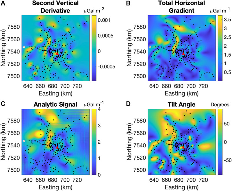
FIGURE 4. Derivative analysis maps of the gravity field at Uturuncu. The red triangle marks the location of Uturuncu, the black dots are gravity measurement locations. (A) Second vertical derivative (LaFehr and Nabighian, 2012) (B) Total horizontal gradient (Cordell, 1979) (C) Analytic signal (Nabighian, 1972) (D) Tilt angle (Miller and Singh, 1994).

4.3 Inversion Results

Figures 5, 6 show the best fit density model for density contrast bounds of ±150 kg m⁻³. These density contrast bounds are roughly midway between the acceptable range of density contrast bounds (see Section 3.2.2). We will refer to this model as the “middle density” model henceforth. Within the range of acceptable density contrast bounds, changing the density contrast bounds mainly affects the connectedness of narrow model features, and the depth extent of some of the deeper features (Figure 5D).

FIGURE 5

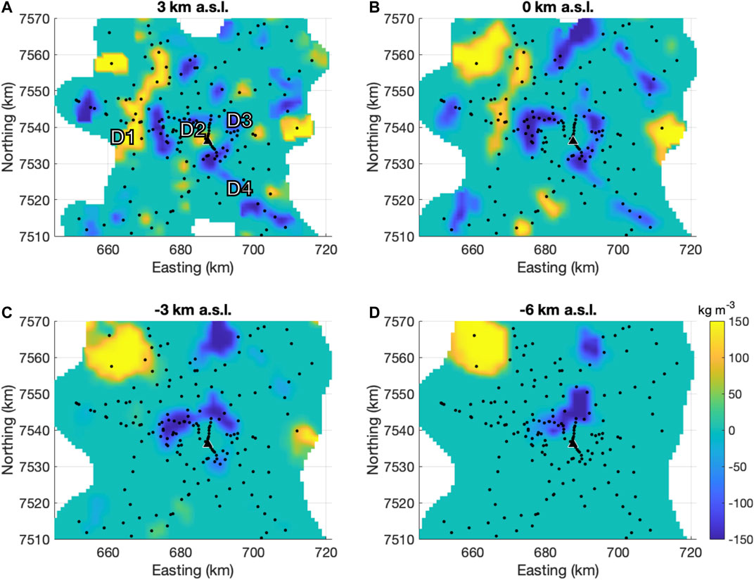
FIGURE 5. Depth slices of the middle density model. Depths are in km above sea level (a.s.l.). Black triangle marks the location of Uturuncu, and black dots are gravity measurement locations used in the inversion.

FIGURE 6

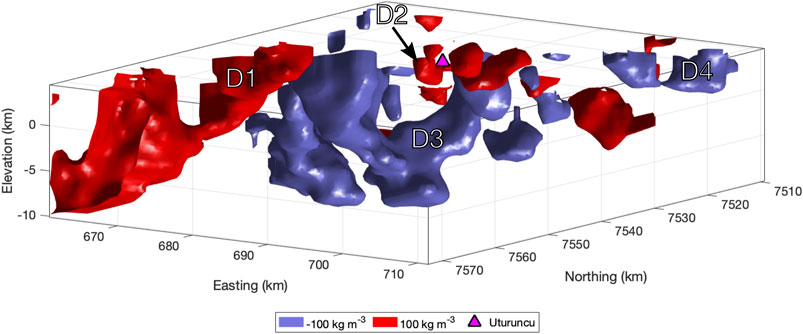
FIGURE 6. ± 100 kg m⁻³ isosurfaces of the middle density model (density contrast bounds = ± 150 kg m⁻³). Model view is upwards from below.

At 3 km a.s.l. (Figure 5A), the most prominent features of the model are a small positive density anomaly below the western flank of Uturuncu (D2), an arc-shaped (or annular in plan view) negative density anomaly centered on Uturuncu (D3), a northeast trending linear positive density anomaly to the northwest of Uturuncu (D1), and a northwest trending negative density anomaly to the southeast of Uturuncu (D4). At sea level (Figure 5B), D2 has disappeared, but all of the other anomalies persist to this depth.

At 3 km below sea level (Figure 5C), D3 is still present, but D1 and the D4 have both disappeared. By 6 km below sea level (Figure 5D), only the northern part of D3 is still present, now with a lobe extending to the north. We note here that there is also a positive density anomaly to the northwest of anomaly D1, present from +3 to −6 km a.s.l. However, as this anomaly is poorly constrained, located on the edge of the survey extent and with lower station coverage, we will not discuss this anomaly further in this paper.

Figure 6 shows the positive and negative density anomalies as isosurfaces of uniform density contrast, with a view angled from below the surface to better display the anomalies. The negative density anomalies surrounding Uturuncu (D3) are the most prominent features in this view, with two “arms” rising from a common base at −6 km a.s.l. to partially surround Uturuncu.

4.4 Verification of Inversion Results

To assess the validity of the inversion results, we performed a bootstrap analysis on the middle density model. Using the same inversion parameters for each run, we re-ran the inversion algorithm 215 times, each time removing a different gravity measurement from the data set. Figure 7 shows the standard deviation of each model cell (interpolated to the same display grid as Figure 5) over the 215 runs of the inversion algorithm.

FIGURE 7

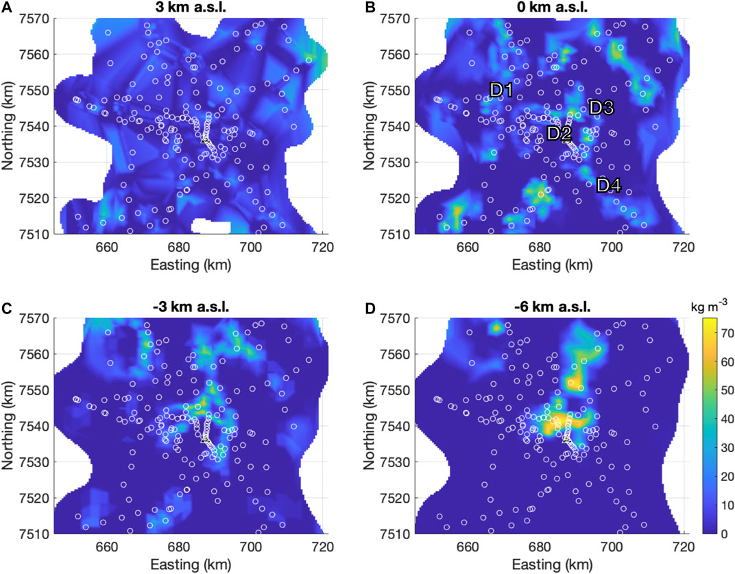
FIGURE 7. Depth slices of the bootstrap sensitivity analysis. Color bar refers to the standard deviation across all models in the analysis. Depths are in km above sea level (a.s.l.). Black triangle marks the location of Uturuncu, and white circles are gravity measurement locations used in the inversion.

For most of the model, the uncertainty ranges from 0 to 10 kg m⁻³, with non-zero uncertainties primarily occurring at the edges of the main density anomalies (Figures 7A-C). Moderate uncertainties (30–50 kg m⁻³) occur at sea level just to the north of Uturuncu, and to the SSW of Uturuncu (Figures 7B,C). The highest uncertainties occur at −6 km a.s.l to the north of Uturuncu (Figure 7D).

5 Discussion

5.1 Interpretation of Density Anomalies

Volcanoes are often associated with a Bouguer gravity anomaly of a similar length scale as the volcanic edifice (Locke et al., 1993; Gudmundsson and Högnadóttir, 2007; Mickus et al., 2007; Barde-Cabusson et al., 2013; Miller and Williams-Jones, 2016; Fernandez-Cordoba et al., 2017; Paoletti et al., 2017), although the level of detail recovered in this study is uncommon for gravity surveys in volcanic areas because of the high spatial observation sampling. Depending on the density contrast between the country rock and volcanic material, the Bouguer anomaly associated with the volcano can either be negative or positive. Negative Bouguer anomalies at larger stratovolcanoes are often interpreted as a magma body (Santos and Rivas, 2009; Camacho et al., 2011; Fernandez-Cordoba et al., 2017). In the case of the Mt Tongariro volcanic massif (New Zealand), Miller and Williams-Jones (2016) interpreted a negative anomaly as a magma feeder system. Positive anomalies are usually interpreted as frozen dike/stock complexes (Locke et al., 1993) or intrusive complexes (Camacho et al., 2007, 2011; Rose et al., 2016) depending on the position and size of the anomalies and their geologic context. As many gravity studies on volcanoes are older with higher uncertainties on positioning (±2 m with geometric/barometric levelling, Rousset et al., 1989), have high uncertainty due to difficult terrain corrections in high relief volcanic landscapes, or both, full 3-D geophysical inversions are rare, and surface inversions or forward modeling approaches are more common methods of analyzing the data. For our study, the relatively high spatial resolution of our gravity data (Figure 1), precise positioning afforded by GNSS instrumentation (Table 1), and the availability of higher precision DEMs (Farr et al., 2007; NASA/METI/AIST/Japan Spacesystems and U.S./Japan ASTER Science Team, 2019) allowed us to go beyond these traditional approaches to perform a full 3-D inversion.

In cases where a 3-D inversion does exist, deeper (>2–5 km) high density anomalies are usually interpreted as intrusive complexes (Camacho et al., 2011) or dike complexes (Camacho et al., 2007). Small, shallow high/positive density anomalies have been explained as lava flows (Miller et al., 2017), domes (Hautmann et al., 2013; Portal et al., 2016), and feeder conduits filed with lava from previous eruptions (Linde et al., 2017). Low density anomalies are often interpreted as pyroclastic materials if shallow (<2–5 km) and/or inside a caldera where low-density caldera infill would be expected (e.g. Barde-Cabusson et al., 2013) or magma if deeper (>2–5 km) (Miller et al., 2017), and often have a columnar geometry.

Arc-shaped features like the one we observe at Uturuncu have been observed at some volcanoes, with the interpretation depending on the polarity of the anomaly. In the context of a caldera, an arc shaped high density anomaly could represent a ring dike along the caldera edge (Barberi et al., 1991; Gudmundsson and Högnadóttir, 2007). Alternatively, at the Somma-Vesuvius volcanic complex in Italy, an older, encircling volcanic edifice produced a high-density arc-shaped anomaly (Linde et al., 2017). Shallow negative/low density arc-shaped anomalies are typically related to tephra, whether on the flanks of the volcano (Bolós et al., 2012; Portal et al., 2016) or infilling a summit crater (Linde et al., 2017).

Similar to other gravity studies at volcanoes and in agreement with previous work by Götze and Kirchner (1997), Prezzi et al. (2009), and del Potro et al. (2013), our study reveals a negative density anomaly beneath Uturuncu (D3 in Figure 5). This negative density anomaly likely represents the upper portion of the columnar negative density anomaly imaged by del Potro et al. (2013), since we are using portions of the same gravity set in our study. del Potro et al. (2013) interpreted the negative density anomaly as a diapir of partial melt, while Gottsmann et al. (2017) and Pritchard et al. (2018) re-interpret the structure as a hybrid column of hydrothermal fluids, solidified dacite, and partially molten dacite (below ca. −6 km a.s.l.). The arc-shaped geometry of D3 is inconsistent with the expected geometry of the top a diapir (Fialko and Pearse, 2012). The lack of evidence for long term deformation at Uturuncu Perkins et al. (2016) also makes a currently active diapir a less likely interpretation.

Fracture zones or a halo of altered volcanic material could be both be consistent with the sign of the D3 density anomaly and the anomaly’s geometry. Fractured material would be lower in density than the surrounding rock. Anomalies D4 and the western portion of D3 (Figures 5A,B) are both aligned NW-SE, similar to a fault mapped by Sparks et al. (2008) and anisotropy measurements by Maher and Kendall (2018). The anisotropy measurements also point to radial anisotropy within 20 km of the Uturuncu edifice (Maher and Kendall, 2018), consistent with the arc-shaped structure. A study of structural lineaments by Walter and Motagh (2014) finds a “fracture girdle” encircling Uturuncu at 15 km from the summit, roughly overlying the imaged negative density anomalies. Alternatively, the negative density contrasts could be explained by a zone of alteration surrounding the volcanic conduit (Sillitoe, 2010; Young et al., 2020). Density measurements of hydrothermally altered rocks in the Kuril–Kamchatka island arc (Frolova et al., 2014) and the Taupo volcanic zone (Wyering et al., 2014) both found that rock density decreased with increasing intensity of alteration. Fumaroles at Uturuncu’s summit point to an active hydrothermal system (Sparks et al., 2008), and Comeau et al. (2016) pointed to magmatic brines as a possible cause for very low resistivity anomalies measured at the same depths as the negative density anomalies. Anomaly D3 may represent an arcuate zone of volcano-tectonic interaction, with fracturing and alteration topping a columnar, mid-crustal magmatic plumbing system (Gottsmann et al., 2017; Pritchard et al., 2018) where fluids from the APMB ultimately reach the surface.

The two positive density anomalies D1 and D2 (Figure 5A) could indicate intrusive rocks, or even areas of sulfide deposition. The depth of D2 beneath Uturuncu is consistent with the depth of the youngest dacite magma erupted at Uturuncu (Muir et al., 2014a), and dacite should be denser than the surrounding country rock at 3 km a.s.l. (Gottsmann et al., 2017). Alternatively, a small, disseminated amount of a very dense material—sulfide mineralization—could also be consistent with the positive density contrasts in our model at D1 and D2. The presence of saline fluids beneath Uturuncu (Comeau et al., 2016) and an active hydrothermal system (Jay et al., 2013) suggest favorable conditions for deposition of ore minerals in the ca 250 kya (Muir et al., 2015) since Uturuncu’s last known eruption (Sillitoe, 2010). Anomaly D1 aligns well with a topographic ridge (Figure 1) formed of older, eroded volcanics (Global Volcanism Program, 2013) and may also represent intrusive rocks and/or a zone of disseminated sulfides.

5.2 Comparison With Resistivity Model

Figure 8 shows the slices of the density model from Figure 5 with overlaid contour lines from the Comeau et al. (2016) resistivity model and relocated earthquake hypocenters (Hudson et al., 2021) from Jay et al. (2012) and Kukarina et al. (2017) measured between April 2009 to 2010 and April 2010 to October 2012, respectively. While structures in both models seem to correspond to one another, with density anomalies seeming to follow or truncate resistivity anomalies, and vice versa, there is no clear one-to-one relationship between resistivity and density. D1 and D2 have opposite resistivity values. D1 aligns well with a high resistivity anomaly (Figure 8B), while D2 matches nearly perfectly with the top of a low resistivity anomaly (Figure 8A). The relationship between density anomaly D3 and the resistivity structures is very complex, with the alternating high and low resistivity anomalies seeming to bend around the low density arc (Figure 8B).

FIGURE 8

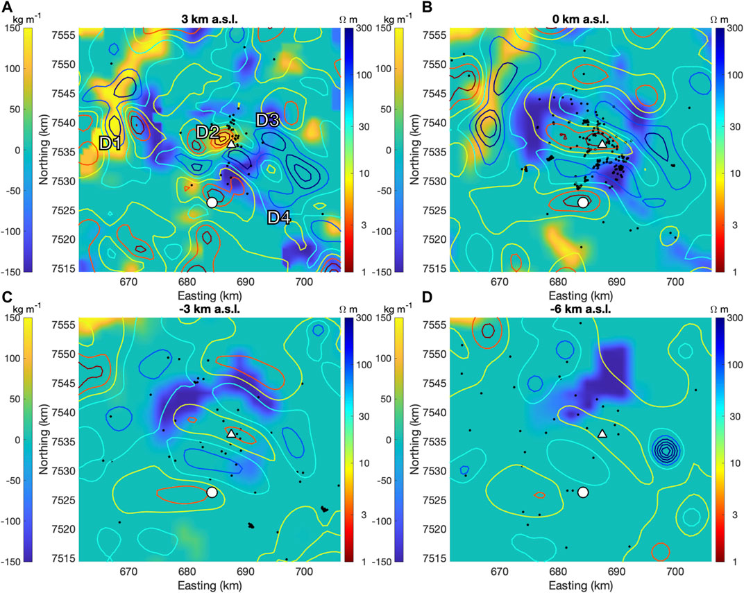
FIGURE 8. Overlay of resistivity model (colored contours) on density model, using same depth slice as in Figure 5. Relocated earthquake hypocenters from previous seismic deployments (Jay et al., 2012; Kukarina et al., 2017; Hudson et al., 2021) within 500 m of the depth slice elevation plotted as black dots. White triangle marks the location of the peak of Uturuncu, and the white circle marks the location of the small subsidence area imaged in Lau et al. (2018) and Eiden et al. (2020).

While the apparent link or correlation between density and resistivity anomaly distributions suggests that both methods highlight the same anomalous subsurface structure, the lack of a one-to-one relationship between density and resistivity likely means that each method is sensitive to different structural properties. Figure 9 attempts to interpret the geophysical anomalies in the resistivity-density space—where variations in resistivity are controlled primarily by the presence and connectedness of conductive materials (brines and sulphides), and density is controlled by the degree of fracturing and the distribution of lithofacies (altered rock vs. disseminated sulfides).

FIGURE 9

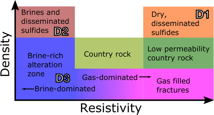
FIGURE 9. Interpretation of models in density-resistivity space. Different colored boxes represent different lithologies in our interpretation. Regions with non-anomalous density and resistivity represent country rock. Regions with low resistivity and high density (D2, Figure 8) we interpret as brines and disseminated sulfides. Regions with high resistivity and low density may represent disseminated sulfides without saline fluids (D1, Figure 8). The low density areas (D3, Figure 8) we interpret as gas filled fractures where resistivity is high, and brine-dominated alteration zones where resistivity is low. Neutral density areas with high resistivity may represent country rock with lower permeability.

In this schematic, areas of low resistivity and high density, such as D2 (Figure 8A), may represent disseminated sulfides (high density) and connected brines (low resistivity). By contrast, the high density, high resistivity anomaly D1 (Figures 8A,B) is best explained by a zone of disseminated sulfides lacking connected brines (high resistivity). The area immediately surrounding Uturuncu (D3, Figure 8B) is likely an active zone of hydrothermal alteration with complex zoning, with zones of gas-filled fractures (low density, high resistivity), brine-rich alteration zones (low to neutral density, low resistivity), and gas-rich alteration zones (low to neutral density, high resistivity). It is also worth noting that the probable source location of a small zone of subsidence south of Uturuncu (Lau et al., 2018) is at the same location as a low resistivity anomaly just south of a branch of D3 (Figure 8B), possibly indicating the presence of brines. Earthquake hypocenters cluster on the edge of D2 and in the area surrounding (Figures 8A,B), and extend from D3 to the location of the shallow subsidence signal Figure 8B), potentially indicating fluid movement. The location of the subsidence on the edge of the arc, as well as the earthquake clusters, suggests that the shallow subsidence may be related to hydrothermal activity, consistent with the interpretations of Lau et al. (2018) and Eiden et al. (2020).

5.3 Exploration of the Density Parameter Space

As a semi-quantitative test of our interpretations of the origin of the subsurface density variations, we can calculate the density contrasts expected for the proposed lithologies in Figure 9, exploring the density contrast parameter space and comparing these spaces with the bounds given by our density modeling. Here we test the following hypotheses for the lithologies of anomalies D3 and D2: negative density contrast anomaly D3 (Figure 8) represents a region of hydrothermal activity consisting of fractures ± saline fluids ± gas ± hydrothermal alteration (Figure 9), and positive density contrast anomaly D2 (Figure 8) represents either a dacite intrusion (Muir et al., 2014a), a zone of disseminated sulfides with brines (Figure 9), or a combination of both. We can falsify any of these hypotheses if we find that combinations of component materials predicted by these hypotheses cannot reproduce the full range of density contrasts we see in our density models.

In these calculations we consider five scenarios (see cartoons in Figure 10) pertaining to these hypotheses and compare them with a “base case” lithology that represents zero density contrast. Since the lithologies in our hypotheses involve a number of different materials, to reduce the dimensionality of the problem we consider only a few components in each scenario. To investigate the hypothesis that anomaly D3 represents a region of hydrothermal activity, in scenario S1 we calculate the density contrasts resulting from gas (high resistivity, low density, Figure 9), saline fluids (low resistivity, low density, Figure 9), or some mixture of the two filling variable amounts of pore space in the rock (Figure 10A). We envision this pore space as secondary porosity in the form of connected fractures, as we would expect hydrothermal activity to increase pore space in existing rock via high pressure fluid injection (Cox, 2016), consistent with the swarm seismicity observed at Uturuncu (Hudson et al., 2021). In scenario S2 pertaining to anomaly D3 we calculate how the extent of chlorite alteration (low resistivity, low density, Figure 9) would affect the density contrast for different amounts of secondary porosity (Figure 10B). To test our hypothesis that anomaly D2 represents either a dacite pluton (Muir et al., 2014a) or a zone of disseminated sulfides (low resistivity, high density, Figure 9), we first consider scenario S3 in which we vary the amount of dacite in the matrix for different amounts of secondary porosity (Figure 10C). As for D3, we assume this area will have some amount of secondary porosity. We then consider scenario S4 in which the positive density contrasts of anomaly D3 are produced by a mixture of disseminated sulfides and saline fluids filling variable amounts of secondary porosity (Figure 10D). We finally investigate scenario S5 in which a mixture of disseminated sulfides and saline fluids fill variable amounts of secondary porosity in a dacite matrix (Figure 10E).

FIGURE 10

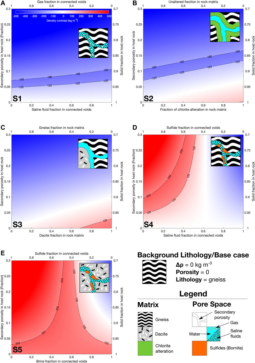
FIGURE 10. Parameter exploration for range of best-fit density contrast models. Fill colors correspond to calculated density contrasts for the combination of components indicated on the x and y axes. The shaded areas in between the black contour lines show the range of acceptable density contrasts (positive = red and negative = blue). Each sub-figure includes an explanatory cartoon, with the components explained in the legend in the lower right hand corner of the main figure. The scenarios explored in the subfigures are as follows: (A) Secondary porosity vs. saline fluid/gas content of pore space (B) Secondary porosity vs extent of chlorite alteration (C) Secondary porosity vs dacite/gneiss in rock matrix (D) Secondary porosity vs sulfide/brine content in gneiss matrix (E) Secondary porosity vs sulfide/brine content in dacite matrix. Scenario numbers from the text are included in the bottom left-hand corner of each subfigure.

Our base case lithology is a paragneiss, metamorphosed sediments with the “Grand Mean” composition proposed for the Central Andean crust by Lucassen et al. (2001). As the anomalies of interest are at greater than 1 km depth, low porosities are appropriate, and for simplicity of calculation we assume zero primary porosity in our base case lithology. We assume a pressure of 45 MPa (hydrostatic pressure at ca. 3.5 km depth, assuming a fluid density of 1,300 kg m⁻³), and a temperature of 250°C, consistent with measurements of gas geochemistry from fumaroles at Uturuncu’s summit (Tobias Fischer, personal communication). The bulk density of the base case lithology is depth dependent according to the depth vs. density curve developed for Uturuncu by Gottsmann et al. (2017). For calculations pertaining to the shallow D2 anomaly and the more vertically extensive D3 anomaly, the base case densities are 2,475 kg m⁻³ and 2,550 kg m⁻³, respectively.

Figure 10 shows the results of our calculations for the scenarios, depicted by the cartoons on the corresponding graph. Table 3 lists the densities of the different materials in each calculation. The fill color in each graph represents the density contrast (same color scale for all graphs). We calculate the density contrast according to Eq. 7, in which Δρ is the density contrast value displayed in the fill colors of the graphs in Figure 10, ϕ is the secondary porosity, ρ_f is the density of the materials (fluids, sulfides, etc.) filling the secondary porosity, ρ_m is the density of the rock matrix (gneiss, alteration, etc.), and ρ₀ is the appropriate base case density. Depending on the scenario, we calculate ρ_f or ρ_m from the densities of two different components ρ₁ and ρ₂ according to Eq. 8, in which X is the fraction of component 1.

$\mathrm{\Delta }\rho =\left[\varphi \cdot {\rho }_f+(1-\varphi )\cdot {\rho }_m\right]-{\rho }_0(7)$

${\rho }_{f,m}=X\cdot {\rho }_1+(1-X)*{\rho }_2(8)$

For all scenarios, we investigate the effect of adding secondary porosity varying from 0 to 30% along the y-axis of the corresponding graph. Along the x axis of each graph we explore the trade-off between two different end-members (described below for each scenario).

TABLE 3

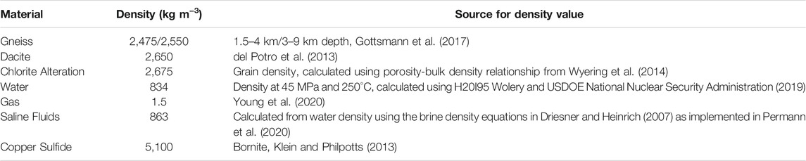
TABLE 3. Density values for parameter space exploration (Figure 10).

Figures 10A,B explore the density contrast parameter space for negative density contrast anomaly D3 (Figures 8, 9). In Figures 10A,B, black contour lines mark the upper and lower density contrast bounds for the negative density contrast anomalies in our models. The blue shaded region between the contour lines corresponds to the range of parameter combinations consistent with our density modeling. Figure 10A shows scenario S1, in which we fill the secondary porosity with a mixture of gas and 3 wt% saline fluid, keeping the matrix as gneiss. The left side of the graph represents 0% saline fluid and 100% gas in the pores, vice versa for the right side of the graph. Figure 10B explores scenario S1, the effect of chlorite alteration on the density contrast, keeping the pore fill as pure water. Chlorite alteration is typical of deeper, high temperature, distal zones surrounding an ore deposit (Sillitoe, 2010; Hervé et al., 2012; Wyering et al., 2014). The left side of Figure 10B represents zero alteration in the rock matrix, and the right side represents 100% alteration of the rock matrix. The density value we use for 100% chlorite alteration (Table 3) is the grain density, i.e., the density of the matrix material, independent of porosity. To calculate this density value, we convert the bulk density of chlorite alteration reported in Wyering et al. (2014) to grain density with the authors’ density-porosity relationship.

Figures 10C–E explore the density contrast parameter space for positive density contrast anomaly D2 (Figures 8, 9). The black contour lines mark the upper and lower density contrast bounds for the positive density contrast anomalies in our models. The red shaded region between the contour lines corresponds to the range of parameter combinations consistent with our density modeling. Figure 10C shows calculations for scenario S3, in which we add a variable amount of dacite to the matrix, keeping the pore fill as pure water. The left side of the graph represents 100% gneiss, and the right side of the graph represents 100% dacite. In Figure 10D for scenario S4 we keep the matrix as gneiss, but explore the density contrast resulting from a mixture of saline fluids and copper sulfides (bornite) in the secondary porosity. Figure 10E for scenario S5 also calculates density contrasts for a mixture of saline fluids and copper sulfides in the pores, but instead considers a purely dacite matrix.

Figure 10 suggests that the negative density contrast anomalies are consistent with any mixture of gas and brine (Figure 10A), and require at least 5% secondary porosity regardless of the amount of alteration in the host rocks (Figure 10B). The amount of secondary porosity required increases with the degree of alteration, which is expected as the minerals formed during chloritization are often denser than the minerals they replace (Sillitoe, 2010; Mathieu, 2018). Further, some amount of fracturing would be required to transport the hydrothermal fluid that initiates the hydrothermal alteration (Hedenquist and Lowenstern, 1994; Sillitoe, 2010; Cox, 2016). Nevertheless, these calculations show that some amount of secondary porosity is required to explain the low density anomalies, consistent with the “fracture girdle” observed by Walter and Motagh (2014) and the anisotropy measurements of Maher and Kendall (2018).

From Figures 10C–E, we observe that while a pure dacite body is insufficiently dense to explain the full range of optimal positive density contrast bounds (Figure 10C), we can explain the positive density contrast anomaly with a disseminated sulfide component. If we assume that the rock matrix is gneiss with no dacite, the sulfide fraction in void spaces could range from 50 to 100%, depending on the porosity (Figure 10D). At low porosities, a dacite matrix permits any amount of sulfide in pore spaces (including none), while at higher porosities the range appears to converge to values near 45% of pore space (Figure 10E).

Although for these calculations we have assumed that the positive density contrast anomaly D2 represents a copper porphyry deposit, we acknowledge that other interpretations may be equally valid. The tectonic environment at Uturuncu does not align well with the tectonic environments of known large Andean copper-porphyry deposits, that are inferred to have formed during periods of intense contraction, along distinct tectonic lineaments (Mpodozis and Cornejo, 2012). An alternative interpretation for D2 could be an epithermal gold deposit, particularly if the D2 anomaly overlies the last intrusion. As gold (15000 kg m⁻³) is much denser than copper sulfides (5,100 kg m⁻³), this means that the ore concentration permitted by our density models would be much smaller compared to a copper sulfide deposit. Additional measurements and analyses are required to conclusively determine the nature and presence of any deposits at Uturuncu, for example, gas geochemistry and multiphase (brine/dacite/sulfides/gas) conductivity forward modeling to determine what sulfide amounts could be consistent with the existing resistivity model (Comeau et al., 2016).

5.4 Error Sources and Limitations of Inversion Method

The quality and distribution of the gravity data, as well as the assumptions and limitations of the inversion method, determine the robustness of the density model. First, the data set used from this inversion is comprised of several different gravity data sets, measured at different times and with different instruments of varying precision, introducing noise of up to 0.1 mGal in the data set. While we have made every effort to tie these data sets together in a consistent manner, we cannot definitively rule out the possibility that significant gravity changes (Poland et al., 2020) due to geological activity occurred in between surveys. However, due to the slow, steady nature of the overall deformation at Uturuncu (Henderson and Pritchard, 2017; Lau et al., 2018), and the lack of any significant changes in unrest between the surveys, large gravity changes are unlikely. For comparison, the largest time-lapse gravity change ever recorded was 1.5 mGal, during the 2018 collapse of the Kilauea caldera (Poland et al., 2020). Time-lapse gravity measurements at Uturuncu between 2010 and 2013 provide no evidence for significant subsurface mass change, as gravity changes are consistent with the free-air gravity change expected from InSAR-measured surface deformation (Gottsmann et al., 2017).

Despite the irregular spatial distribution of the observations, an unavoidable consequence of the rugged terrain, the main features of our model are robust. The GROWTH 2.0 inversion algorithm does account for irregularly spaced observations by limiting the model domain and scaling cell sizes by the sensitivity of the observation network (Camacho et al., 2011). However, in general small scale (<5 km) features in areas of low station coverage are not reliable features of the model. The bootstrap uncertainty analysis of the model (Figure 7) gives us confidence in the main features of the model, even given the irregular measurement distribution and the noise in the data, as the main anomalies typically show significant variability only on their edges. The deeper portions of some of the anomalies do show higher levels of variability in the analysis (Figure 5), likely due to the expected diminishing sensitivity of gravity data at depth.

The GROWTH 2.0 inversion algorithm (Camacho et al., 2011) also introduces certain limitations. Of primary importance is the “strong” assumption of the algorithm that all anomalies have a uniform density contrast (Camacho et al., 2000), a vast oversimplification of geological realities. In addition, there is likely a non-zero background density increase with depth at Uturuncu (Gottsmann et al., 2017), a condition we were not able to successfully account for in our inversions, due to limitations with the software. However, even with these limitations, the main density anomalies recovered with the inversion match those highlighted by the gradient analysis of the data to a striking degree (Figures 4, 5), giving us confidence that the inversion is recovering features actually present in the data.

Our density model is further validated by other independent datasets at Uturuncu. The striking correspondence between the resistivity and density anomalies is a strong argument for the existence of the features in the density model (Figure 8). Positive density anomaly D2 overlaps with the storage depth of the last dacite erupted at Uturuncu (Muir et al., 2014a). Radial anisotropy (Maher and Kendall, 2018) and lineaments (Walter and Motagh, 2014) align well with low density anomaly D3 (Figure 5) surrounding the base of Uturuncu, together pointing to a zone of fracturing surrounding Uturuncu. The main features of our density model correspond well to existing knowledge of Uturuncu’s structure, giving us confidence in our results and interpretations.

5.5 Shallow Structure at Uturuncu

Figure 11 shows a conceptual model of the shallow structure at Uturuncu, overlain on a cross section of the density and resistivity models. In this model we have a shallow zone of sulfide deposition at 3 km a.s.l. with abundant brines (high density, low resistivity). Surrounding and beneath the sulfide deposition zone is a halo of hydrothermal activity and alteration, with both vapor and fluid dominated zones (low density, high and low resistivity), with clusters of earthquakes possibly representing active fluid movement.

FIGURE 11

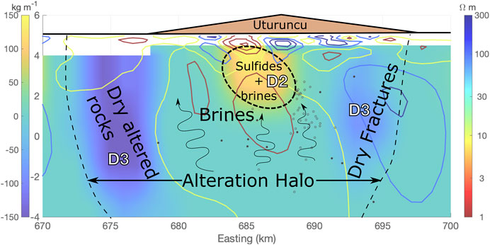
FIGURE 11. Conceptual model of subsurface structure at Uturuncu from joint interpretation of density and resistivity models. The cross section cuts W-E at the peak of Uturuncu (Northing = 7,536), with the resistivity model (colored contours) overlaid on the density model as in Figure 8. Small circles represent earthquake hypocenters within 500 m of the slice from Hudson et al. (2021). An alteration halo consisting of brines (low resistivity, negative to neutral density contrast), altered rocks (low density), brines (low resistivity), and dry fractures (negative density contrast, high resistivity) surrounds a shallow zone of sulfide deposition (low resistivity, positive density contrast) beneath Uturuncu. Arrows indicate possible fluid movement, inferred from earthquake locations, in zones with brines.

5.6 Implications for the Life-Cycle of Volcanism at Uturuncu

As we see no evidence for shallow accumulations of melt, we do not consider it likely that Uturuncu will erupt again in the near future, or that the deformation at Uturuncu is due to the transfer of molten material. Rather, we posit that the geophysical evidence here is more indicative of the periodic release of hydrothermal fluids in a slowly cooling magmatic system that has ceased active eruption. Afanasyev et al. (2018) finds that formation of a magmatic brine lens from phase separation of super-critical magmatic fluids may explain the low resistivity anomalies imaged beneath several volcanoes, including Uturuncu. The low density anomaly (D3) we image between +3 and −3 km a.s.l., the same depth as the low resistivity anomalies, would be consistent with high permeability zones with brines.

Rather than a rejuvenating magmatic system, Uturuncu may instead represent the waning stages of the volcanic life cycle, with the deformation, seismic, degassing and other activity observed at Uturuncu related to ore formation. Cox (2016) proposes that hydrothermal ore deposits may form through geologically short intervals of injection-driven swarm seismicity. Blundy et al. (2015) also suggest that porphyry-copper deposits, abundant in this region of the Andes (Sillitoe, 2010), are formed through multiple pulses of hydrothermal fluids. Recent work on the seismic catalog at Uturuncu suggests that the seismicity at Uturuncu may be closer to fluid movements than first calculated (Hudson et al., 2021). Seismicity related to fluids, a lack of geomorphological evidence for permanent deformation (Perkins et al., 2016), and subsurface geophysical imaging that points to fracturing and brines rather than magma, may indicate that the deformation observed at Uturuncu is due to an episodic pulse of magmatic fluids released from a cooling magmatic system, similar to the model in Gottsmann et al. (2017) of magma mush reorganization. The shallow high density body could possibly represent the beginnings of an ore body, as high density, sulfide deposits with connected brines would be consistent with the high density and low resistivity anomalies imaged in this area. However, further analysis of the gasses from the fumaroles at Uturuncu could refute this hypothesis, if the chemistry of the gasses is inconsistent with ore formation (Blundy et al., 2015).

5.7 Imaging Hydrothermal and Magmatic Systems

This study shows the importance of using multiple complementary geophysical methods when imaging hydrothermal and magmatic systems, as each method will highlight different features of a common structure. Viewed separately, the resistivity and density models at Uturuncu appear to show different structures, potentially leading to very different interpretations of the shallow portion of the trans-crustal magma system at Uturuncu. However, viewed together, each method refines the picture of volcanic structure provided by the other, leading to a more holistic view of the hydrothermal system. The close correspondence in structure between the density and resistivity models was a surprising and unexpected outcome of the comparison. Future joint inversions of these two datasets would be valuable to understand what additional information joint inversion can provide beyond a simple overlaying of the models.

Such intensive geophysical imaging of Pleistocene volcanoes is rare—and for good reason, as Holocene volcanoes are typically more likely to pose a significant hazard to human life. However, systems like Uturuncu and Lazufre (Pritchard et al., 2018) demonstrate that even older volcanic systems can show signs of life. Understanding the subsurface structures of these “zombie” volcanoes is critical to understanding the potential causes of this unrest, to be able to distinguish shallow accumulation of magma from a complex hydrothermal system more indicative of the post-eruptive stage in the life-cycle of a volcano. More multi-parameter geophysical studies like the work conducted at Uturuncu and Lazufre are needed to understand to what extent these systems are unique outliers or simply members of an under-studied stage of volcanic activity.

6 Conclusion

In this paper we present an updated gravity data set at Uturuncu with increased resolution in the upper 10 km of the crust. Gradient analysis and inversion both reveal several density anomalies of interest, including positive anomalies directly beneath and to the northwest of Uturuncu, an arc-shaped negative anomaly surrounding the positive anomaly beneath Uturuncu, and a NW-SE trending linear negative anomaly to the southeast of Uturuncu. These density anomalies have a complex correspondence to the resistivity model from Comeau et al. (2016), with no clear one-to-one relationship between density and resistivity. However, the two models show structural similarities that suggest they are revealing the same structures. We interpret the high density, low resistivity anomaly beneath Uturuncu as a zone of sulfide deposition with connected brines, and the high density, high resistivity anomaly to the northwest of Uturuncu as an area of dry disseminated sulfides. The low density arc surrounding the high density, low resistivity anomaly is likely an alteration halo, with varying degrees of gas, brines, altered rock, and dry fractures. The geophysical anomalies at Uturuncu may therefore represent the waning of volcanic activity and the beginning of ore body formation, with a low potential for eruption in the near future. The rich dataset available at Uturuncu is a unique case in which we have detailed imaging of a trans-crustal magma system from the base of the crust to the shallow hydrothermal system, and is one of only a few Pleistocene age “zombie” systems with this level of imaging. Future multi-parameter studies of similar trans-crustal magma systems will be valuable for evaluating hazard potential and the distribution of fluids at these systems, as well as gaining useful knowledge for mineral exploration.

Data Availability Statement

The datasets presented in this study can be found in online repositories. The names of the repository/repositories and accession number(s) can be found below: Zenodo Repository: https://zenodo.org/record/4959159.

Author Contributions

JG and MP conceived the project underpinning the research and secured funding (NERC grant NE/S008845/1 and NSF grant 1757495). PM wrote the initial draft, analyzed the data (inversion, derivative analysis, joint analysis), and secured additional funding (FINESST award number 80NSSC19K1339). JG collected the gravity and GNSS data together with NY, FT, ET, and RT, post-processed the data, and performed the gravity data reductions. All authors contributed to the discussion and interpretation of the findings. The writing of the final draft was led by PM with contributions from JG and MP.

Funding

PM was supported by NASA FINESST award number 80NSSC19K1339. MP and PM were both supported by NSF grant number 1757495. JG and NY were supported by NERC grant number NE/S008845/1. FT, RT, and ET were jointly supported by NSF grant 1757495 and NERC grant NE/S008845/1.

Conflict of Interest

The authors declare that the research was conducted in the absence of any commercial or financial relationships that could be construed as a potential conflict of interest.

Publisher’s Note

All claims expressed in this article are solely those of the authors and do not necessarily represent those of their affiliated organizations, or those of the publisher, the editors and the reviewers. Any product that may be evaluated in this article, or claim that may be made by its manufacturer, is not guaranteed or endorsed by the publisher.

Acknowledgments

Thank you to editors Valerio Acocella, Roberto Sulpizio, and reviewers Eisuke Fujita and Micol Todesco for their comments and suggestions that greatly improved the quality of this manuscript. We would like to thank the San Calixto Observatory and Servicio Nacional de Áreas Protegidas de Bolivia for their support of this research. We would also like to thank Jeff MacQueen, Matthew Comeau, Michael Kendall, Thomas Hudson, Jon Blundy, and Martyn Unsworth for many helpful discussions and comments.

References

Afanasyev, A., Blundy, J., Melnik, O., and Sparks, S. (2018). Formation of Magmatic Brine Lenses via Focussed Fluid-Flow beneath Volcanoes. Earth Planet. Sci. Lett. 486, 119–128. doi:10.1016/j.epsl.2018.01.013

CrossRef Full Text | Google Scholar

Aizawa, K., Yoshimura, R., Oshiman, N., Yamazaki, K., Uto, T., Ogawa, Y., et al. (2005). Hydrothermal System beneath Mt. Fuji Volcano Inferred from Magnetotellurics and Electric Self-Potential. Earth Planet. Sci. Lett. 235, 343–355. doi:10.1016/j.epsl.2005.03.023

CrossRef Full Text | Google Scholar

Allmendinger, R. W., Jordan, T. E., Kay, S. M., and Isacks, B. L. (1997). The Evolution of the Altiplano-Puna Plateau of the Central Andes. Annu. Rev. Earth Planet. Sci. 25, 139–174. doi:10.1146/annurev.earth.25.1.139

CrossRef Full Text | Google Scholar

Barazangi, M., and Isacks, B. L. (1976). Spatial Distribution of Earthquakes and Subduction of the Nazca Plate beneath South America. Geol 4, 686–692. doi:10.1130/0091-7613(1976)4<686:sdoeas>2.0.co;2

CrossRef Full Text | Google Scholar

Barberi, F., Cassano, E., La Torre, P., and Sbrana, A. (1991). Structural Evolution of Campi Flegrei Caldera in Light of Volcanological and Geophysical Data. J. Volcanology Geothermal Res. 48, 33–49. doi:10.1016/0377-0273(91)90031-T

CrossRef Full Text | Google Scholar

Barde-Cabusson, S., Gottsmann, J., Martí, J., Bolós, X., Camacho, A. G., Geyer, A., et al. (2013). Structural Control of Monogenetic Volcanism in the Garrotxa Volcanic Field (Northeastern Spain) from Gravity and Self-Potential Measurements. Bull. Volcanol 76, 788. doi:10.1007/s00445-013-0788-0

CrossRef Full Text | Google Scholar

Blundy, J., Mavrogenes, J., Tattitch, B., Sparks, S., and Gilmer, A. (2015). Generation of Porphyry Copper Deposits by Gas-Brine Reaction in Volcanic Arcs. Nat. Geosci 8, 235–240. doi:10.1038/ngeo2351

CrossRef Full Text | Google Scholar

Bolós, X., Barde-Cabusson, S., Pedrazzi, D., Martí, J., Casas, A., Himi, M., et al. (2012). Investigation of the inner structure of La Crosa de Sant Dalmai maar (Catalan Volcanic Zone, Spain). J. Volcanology Geothermal Res. 247-248, 37–48. doi:10.1016/j.jvolgeores.2012.08.003

CrossRef Full Text | Google Scholar

Camacho, A. G., Fernández, J., and Gottsmann, J. (2011). The 3-D Gravity Inversion Package GROWTH2.0 and its Application to Tenerife Island, Spain. Comput. Geosciences 37, 621–633. doi:10.1016/j.cageo.2010.12.003

CrossRef Full Text | Google Scholar

Camacho, A. G., Montesinos, F. G., and Vieira, R. (2000). Gravity Inversion by Means of Growing Bodies. GEOPHYSICS 65, 95–101. doi:10.1190/1.1444729

CrossRef Full Text | Google Scholar

Camacho, A. G., Nunes, J. C., Ortiz, E., França, Z., and Vieira, R. (2007). Gravimetric Determination of an Intrusive Complex under the Island of Faial (Azores): Some Methodological Improvements. Geophys. J. Int. 171, 478–494. doi:10.1111/j.1365-246X.2007.03539.x

CrossRef Full Text | Google Scholar

Chirokov, A. (2020). Scattered Data Interpolation and Approximation Using Radial Base Functions. MATLAB Central File Exchange.

Cladouhos, T. T., Allmendinger, R. W., Coira, B., and Farrar, E. (1994). Late Cenozoic Deformation in the Central Andes: Fault Kinematics from the Northern Puna, Northwestern Argentina and Southwestern Bolivia. J. South Am. Earth Sci. 7, 209–228. doi:10.1016/0895-9811(94)90008-6

CrossRef Full Text | Google Scholar

Clavero, J. E., Sparks, R. S. J., Pringle, M. S., Polanco, E., and Gardeweg, M. C. (2004). Evolution and Volcanic Hazards of Taapaca Volcanic Complex, Central Andes of Northern Chile. J. Geol. Soc. 161, 603–618. doi:10.1144/0016-764902-065

CrossRef Full Text | Google Scholar

Comeau, M. J., Unsworth, M. J., and Cordell, D. (2016). New Constraints on the Magma Distribution and Composition beneath Volcán Uturuncu and the Southern Bolivian Altiplano from Magnetotelluric Data. Geosphere 12, 1391–1421. doi:10.1130/GES01277.1

CrossRef Full Text | Google Scholar

Cordell, L. (1979). “Gravimetric Expression of Graben Faulting in Santa Fe Country and the Espanola Basin,” in 30th Field Conference (New Mexico: Geological Society, 59–64.

Google Scholar

Cox, S. F. (2016). Injection-Driven Swarm Seismicity and Permeability Enhancement: Implications for the Dynamics of Hydrothermal Ore Systems in High Fluid-Flux, Overpressured Faulting Regimes-An Invited Paper. Econ. Geology. 111, 559–587. doi:10.2113/econgeo.111.3.559

CrossRef Full Text | Google Scholar

de Silva, S. L. (1989). Altiplano-Puna Volcanic Complex of the central Andes. Geol 17, 1102–1106. doi:10.1130/0091-7613(1989)017<1102:APVCOT>2.3.CO;2

CrossRef Full Text | Google Scholar

Dehant, V., Defraigne, P., and Wahr, J. M. (1999). Tides for a Convective Earth. J. Geophys. Res. 104, 1035–1058. doi:10.1029/1998JB900051

CrossRef Full Text | Google Scholar

del Potro, R., Díez, M., Blundy, J., Camacho, A. G., and Gottsmann, J. (2013). Diapiric Ascent of Silicic Magma beneath the Bolivian Altiplano. Geophys. Res. Lett. 40, 2044–2048. doi:10.1002/grl.50493

CrossRef Full Text | Google Scholar

Driesner, T., and Heinrich, C. A. (2007). The System H2O-NaCl. Part I: Correlation Formulae for Phase Relations in Temperature-Pressure-Composition Space from 0 to 1000°C, 0 to 5000bar, and 0 to 1 XNaCl. Geochimica et Cosmochimica Acta 71, 4880–4901. doi:10.1016/j.gca.2006.01.033

CrossRef Full Text | Google Scholar

Ebmeier, S. K., Andrews, B. J., Araya, M. C., Arnold, D. W. D., Biggs, J., Cooper, C., et al. (2018). Synthesis of Global Satellite Observations of Magmatic and Volcanic Deformation: Implications for Volcano Monitoring & the Lateral Extent of Magmatic Domains. J. Appl. Volcanol. 7, 2. doi:10.1186/s13617-018-0071-3

CrossRef Full Text | Google Scholar

Eiden, E., MacQueen, P., Henderson, S. T., and Pritchard, M. E. (2020). “Investigating Hydrothermal and Magmatic Deformation Using Geodetic Time Series at Uturuncu Volcano, Bolivia,” in AGU Fall Meeting 2020, online/virtual conference (AGU).

Google Scholar

Farr, T. G., Rosen, P. A., Caro, E., Crippen, R., Duren, R., Hensley, S., et al. (2007). The Shuttle Radar Topography Mission. Rev. Geophys. 45, 1–31. doi:10.1029/2005RG000183

CrossRef Full Text | Google Scholar

Fernandez-Cordoba, J., Zamora-Camacho, A., and Espindola, J. M. (2017). Gravity Survey at the Ceboruco Volcano Area (Nayarit, Mexico): A 3-D Model of the Subsurface Structure. Pure Appl. Geophys. 174, 3905–3918. doi:10.1007/s00024-017-1600-4

CrossRef Full Text | Google Scholar

Fialko, Y., and Pearse, J. (2012). Sombrero Uplift above the Altiplano-Puna Magma Body: Evidence of a Ballooning Mid-crustal Diapir. Science 338, 250–252. doi:10.1126/science.1226358

PubMed Abstract | CrossRef Full Text | Google Scholar

Fournier, N., and Chardot, L. (2012). Understanding Volcano Hydrothermal Unrest from Geodetic Observations: Insights from Numerical Modeling and Application to White Island Volcano, New Zealand. J. Geophys. Res. 117, a–n. doi:10.1029/2012JB009469

CrossRef Full Text | Google Scholar

Giambiagi, L., Alvarez, P., and Spagnotto, S. (2016). Temporal Variation of the Stress Field during the Construction of the central Andes: Constrains from the Volcanic Arc Region (22-26°S), Western Cordillera, Chile, during the Last 20 Ma. Tectonics 35, 2014–2033. doi:10.1002/2016TC004201

CrossRef Full Text | Google Scholar

Gioncada, A., Vezzoli, L., Mazzuoli, R., Omarini, R., Nonnotte, P., and Guillou, H. (2010). Pliocene Intraplate-type Volcanism in the Andean Foreland at 26°10′S, 64°40′W (NW Argentina): Implications for Magmatic and Structural Evolution of the Central Andes. Lithosphere 2, 153–171. doi:10.1130/L81.1

CrossRef Full Text | Google Scholar

Global Volcanism Program (2013). Volcanoes of the World. Washington, DC: Smithsonian Institution. v. 4.8.0.

Gottsmann, J., Blundy, J., Henderson, S., Pritchard, M. E., and Sparks, R. S. J. (2017). Thermomechanical Modeling of the Altiplano-Puna Deformation Anomaly: Multiparameter Insights into Magma Mush Reorganization. Geosphere 13, GES01420.1–1065. doi:10.1130/GES01420.1

CrossRef Full Text | Google Scholar

Gottsmann, J., del Potro, R., and Muller, C. (2018). 50 Years of Steady Ground Deformation in the Altiplano-Puna Region of Southern Bolivia. Geosphere 14, 65–73. doi:10.1130/GES01570.1

CrossRef Full Text | Google Scholar

Götze, H.-J., and Kirchner, A. (1997). Interpretation of Gravity and Geoid in the Central Andes between 20° and 29° S. J. South Am. Earth Sci. 10, 179–188. doi:10.1016/S0895-9811(97)00014-X

CrossRef Full Text | Google Scholar

Götze, H.-J., Lahmeyer, B., Schmidt, S., Strunk, S., and Araneda, M. (1990). Central Andes Gravity Data Base. Eos Trans. AGU 71, 401–407. doi:10.1029/90EO00148

CrossRef Full Text | Google Scholar

Gudmundsson, M. T., and Högnadóttir, T. (2007). Volcanic Systems and Calderas in the Vatnajökull Region, central Iceland: Constraints on Crustal Structure from Gravity Data. J. Geodynamics 43, 153–169. doi:10.1016/j.jog.2006.09.015

CrossRef Full Text | Google Scholar

Hammer, S. (1939). Terrain Corrections for Gravimeter Stations. GEOPHYSICS 4, 184–194. doi:10.1190/1.1440495

CrossRef Full Text | Google Scholar

Hautmann, S., Camacho, A. G., Gottsmann, J., Odbert, H. M., and Syers, R. T. (2013). The Shallow Structure beneath Montserrat (West Indies) from New Bouguer Gravity Data. Geophys. Res. Lett. 40, 5113–5118. doi:10.1002/grl.51003

CrossRef Full Text | Google Scholar

Hedenquist, J. W., and Lowenstern, J. B. (1994). The Role of Magmas in the Formation of Hydrothermal Ore Deposits. Nature 370, 519–527. doi:10.1038/370519a0

CrossRef Full Text | Google Scholar

Henderson, S. T., and Pritchard, M. E. (2013). Decadal Volcanic Deformation in the Central Andes Volcanic Zone Revealed by InSAR Time Series. Geochem. Geophys. Geosyst. 14, 1358–1374. doi:10.1002/ggge.20074

CrossRef Full Text | Google Scholar

Henderson, S. T., and Pritchard, M. E. (2017). Time-dependent Deformation of Uturuncu Volcano, Bolivia, Constrained by GPS and InSAR Measurements and Implications for Source Models. Geosphere 13, 1834–1854. doi:10.1130/GES01203.1

CrossRef Full Text | Google Scholar

Hervé, M., Sillitoe, R. H., Wong, C., Fernández, P., Crignola, F., Ipinza, M., et al. (2012). Geologic Overview of the Escondida Porphyry Copper District, Northern Chile. Littleton, CO: Society of Economic Geologists Special Publication. 16, 55–78.

Hudson, T. S., Kendall, M., Pritchard, M., Blundy, J. D., and Gottsmann, J. H. (2021). From Slab to Surface: Earthquake Evidence for Fluid Migration at Uturuncu Volcano. Earth Space Sci. Open Archive, 39, 1–39. doi:10.1002/essoar.10506629.1

CrossRef Full Text | Google Scholar

Jay, J. A., Pritchard, M. E., West, M. E., Christensen, D., Haney, M., Minaya, E., et al. (2012). Shallow Seismicity, Triggered Seismicity, and Ambient Noise Tomography at the Long-Dormant Uturuncu Volcano, Bolivia. Bull. Volcanol 74, 817–837. doi:10.1007/s00445-011-0568-7

CrossRef Full Text | Google Scholar

Jay, J. A., Welch, M., Pritchard, M. E., Mares, P. J., Mnich, M. E., Melkonian, A. K., et al. (2013). Volcanic Hotspots of the central and Southern Andes as Seen from Space by ASTER and MODVOLC between the Years 2000 and 2010. Geol. Soc. Lond. Spec. Publications 380, 161–185. doi:10.1144/SP380.1

CrossRef Full Text | Google Scholar

Julia, F., Vladimir, L., Sergey, R., and David, Z. (2014). Effects of Hydrothermal Alterations on Physical and Mechanical Properties of Rocks in the Kuril-Kamchatka Island Arc. Eng. Geology. 183, 80–95. doi:10.1016/j.enggeo.2014.10.011

CrossRef Full Text | Google Scholar

Kay, S. M., and Coira, B. L. (2009). Shallowing and Steepening Subduction Zones, continental Lithospheric Loss, Magmatism, and Crustalflow under the Central Andean Altiplano-Puna Plateau. Backbone of the Americas: shallow subduction, plateau uplift, and ridge and terrane collision 204, 229. doi:10.1130/2009.1204(11)

CrossRef Full Text | Google Scholar

Klein, C., and Philpotts, A. R. (2013). Earth Materials: Introduction to Mineralogy and Petrology. Cambridge University Press.

Kukarina, E., West, M., Keyson, L. H., Koulakov, I., Tsibizov, L., and Smirnov, S. (2017). Focused Magmatism beneath Uturuncu Volcano, Bolivia: Insights from Seismic Tomography and Deformation Modeling. Geosphere 13, 1855–1866. doi:10.1130/ges01403.1

CrossRef Full Text | Google Scholar

LaFehr, T. R., and Nabighian, M. N. (2012). Fundamentals of Gravity Exploration. Tulsa, OK: Geophysical Monograph Series (Society of Exploration Geophysicists. doi:10.1190/1.9781560803058

CrossRef Full Text

Lau, N., Tymofyeyeva, E., and Fialko, Y. (2018). Variations in the Long-Term Uplift Rate Due to the Altiplano-Puna Magma Body Observed with Sentinel-1 Interferometry. Earth Planet. Sci. Lett. 491, 43–47. doi:10.1016/j.epsl.2018.03.026

CrossRef Full Text | Google Scholar

Linde, N., Ricci, T., Baron, L., Shakas, A., and Berrino, G. (2017). The 3-D Structure of the Somma-Vesuvius Volcanic Complex (Italy) Inferred from New and Historic Gravimetric Data. Sci. Rep. 7, 8434. doi:10.1038/s41598-017-07496-y

PubMed Abstract | CrossRef Full Text | Google Scholar

Locke, C. A., Cassidy, J., and MacDonald, A. (1993). Three-dimensional Structure of Relict Stratovolcanoes in Taranaki, New Zealand: Evidence from Gravity Data. J. volcanology geothermal Res. 59, 121–130. doi:10.1016/0377-0273(93)90081-2

CrossRef Full Text | Google Scholar

Lucassen, F., Becchio, R., Harmon, R., Kasemann, S., Franz, G., Trumbull, R., et al. (2001). Composition and Density Model of the continental Crust at an Active continental Margin-The Central Andes between 21° and 27°S. Tectonophysics 341, 195–223. doi:10.1016/S0040-1951(01)00188-3

CrossRef Full Text | Google Scholar

Maher, S., and Kendall, J.-M. (2018). Crustal Anisotropy and State of Stress at Uturuncu Volcano, Bolivia, from Shear-Wave Splitting Measurements and Magnitude-Frequency Distributions in Seismicity. Earth Planet. Sci. Lett. 495, 38–49. doi:10.1016/j.epsl.2018.04.060

CrossRef Full Text | Google Scholar

Mathieu, L. (2018). Quantifying Hydrothermal Alteration: A Review of Methods. Geosciences 8, 245. doi:10.3390/geosciences8070245

CrossRef Full Text | Google Scholar

McFarlin, H., Christensen, D., McNutt, S. R., Ward, K. M., Ryan, J., Zandt, G., et al. (2018). Receiver Function Analyses of Uturuncu Volcano, Bolivia and Vicinity. Geosphere 14, 50–64. doi:10.1130/GES01560.1

CrossRef Full Text | Google Scholar

Mickus, K., Tadesse, K., Keller, G. R., and Oluma, B. (2007). Gravity Analysis of the Main Ethiopian Rift. J. Afr. Earth Sci. 48, 59–69. doi:10.1016/j.jafrearsci.2007.02.008

CrossRef Full Text | Google Scholar

Miller, C. A., Williams-Jones, G., Fournier, D., and Witter, J. (2017). 3D gravity inversion and thermodynamic modelling reveal properties of shallow silicic magma reservoir beneath Laguna del Maule, Chile. Earth Planet. Sci. Lett. 459, 14–27. doi:10.1016/j.epsl.2016.11.007

CrossRef Full Text | Google Scholar

Miller, C. A., and Williams-Jones, G. (2016). Internal Structure and Volcanic hazard Potential of Mt Tongariro, New Zealand, from 3D Gravity and Magnetic Models. J. Volcanology Geothermal Res. 319, 12–28. doi:10.1016/j.jvolgeores.2016.03.012

CrossRef Full Text | Google Scholar

Miller, H. G., and Singh, V. (1994). Potential Field Tilt-A New Concept for Location of Potential Field Sources. J. Appl. Geophys. 32, 213–217. doi:10.1016/0926-9851(94)90022-1

CrossRef Full Text | Google Scholar

Mpodozis, C., and Cornejo, P. (2012). Cenozoic Tectonics and Porphyry Copper Systems of the Chilean Andes. Littleton, CO: Society of Economic Geologists Special Publication. 16, 329–360. doi:10.5382/sp.16.14

CrossRef Full Text

Muir, D. D., Barfod, D. N., Blundy, J. D., Rust, A. C., Sparks, R. S. J., and Clarke, K. M. (2015). The Temporal Record of Magmatism at Cerro Uturuncu, Bolivian Altiplano. Geol. Soc. Lond. Spec. Publications 422, 57–83. doi:10.1144/SP422.1

CrossRef Full Text | Google Scholar

Muir, D. D., Blundy, J. D., Hutchinson, M. C., and Rust, A. C. (2014a). Petrological Imaging of an Active Pluton beneath Cerro Uturuncu, Bolivia. Contrib. Mineral. Petrol. 167, 980. doi:10.1007/s00410-014-0980-z

CrossRef Full Text | Google Scholar

Muir, D. D., Blundy, J. D., Rust, A. C., and Hickey, J. (2014b). Experimental Constraints on Dacite Pre-eruptive Magma Storage Conditions beneath Uturuncu Volcano. J. Petrol. 55, 749–767. doi:10.1093/petrology/egu005

CrossRef Full Text | Google Scholar

Nabighian, M. N. (1972). The Analytic Signal of Two‐dimensional Magnetic Bodies with Polygonal Cross‐section: Its Properties and Use for Automated Anomaly Interpretation. Geophysics 37, 507–517. doi:10.1190/1.1440276

CrossRef Full Text | Google Scholar

NASA/METI/AIST/Japan Spacesystems, and U.S./Japan ASTER Science Team (2019). ASTER Global Digital Elevation Model V003. Available at: https://lpdaac.usgs.gov/products/astgtmv003/

Paoletti, V., Fedi, M., and Florio, G. (2017). The Structure of the Ischia Volcanic Island from Magnetic and Gravity Data. Ann. Geophys. 60, GM674. doi:10.4401/ag-7550

CrossRef Full Text | Google Scholar

Pareja, L. J., and Ballón, A. R. (1978). Mapa geológico de Bolivia.

Perkins, J. P., Finnegan, N. J., Henderson, S. T., and Rittenour, T. M. (2016). Topographic Constraints on Magma Accumulation below the Actively Uplifting Uturuncu and Lazufre Volcanic Centers in the Central Andes. Geosphere 12, 1078–1096. doi:10.1130/GES01278.1

CrossRef Full Text | Google Scholar

Permann, C. J., Gaston, D. R., Andrš, D., Carlsen, R. W., Kong, F., Lindsay, A. D., et al. (2020). MOOSE: Enabling Massively Parallel Multiphysics Simulation. SoftwareX 11, 100430. doi:10.1016/j.softx.2020.100430

CrossRef Full Text | Google Scholar

Poland, M. P., Carbone, D., and Patrick, M. R. (2020). “The Largest Gravity Changes Ever Recorded: Continuous Gravity Monitoring of the Onset of Kīlauea’s 2018 Eruption,” in AGU Fall Meeting 2020 (AGU).

Google Scholar

Portal, A., Gailler, L.-S., Labazuy, P., and Lénat, J.-F. (2016). Geophysical Imaging of the Inner Structure of a Lava Dome and its Environment through Gravimetry and Magnetism. J. Volcanology Geothermal Res. 320, 88–99. doi:10.1016/j.jvolgeores.2016.04.012

CrossRef Full Text | Google Scholar

Prezzi, C. B., Götze, H.-J., and Schmidt, S. (2009). 3D Density Model of the Central Andes. Phys. Earth Planet. Interiors 177, 217–234. doi:10.1016/j.pepi.2009.09.004

CrossRef Full Text | Google Scholar

Pritchard, M. E., de Silva, S. L., Michelfelder, G., Zandt, G., McNutt, S. R., Gottsmann, J., et al. (2018). Synthesis: PLUTONS: Investigating the Relationship between Pluton Growth and Volcanism in the Central Andes. Geosphere 14, 954–982. doi:10.1130/GES01578.1

CrossRef Full Text | Google Scholar

Pritchard, M. E., Furtney, M., and Cooper, J. (2014). VGP Spotlight: Is a Zombie Volcano a Thing?. Available at: https://connect.agu.org/vgp/vgp-resources/vgp-spotlight-features/vgp-spotlight-is-a-zombie-volcano-a-thing

Pritchard, M. E., and Simons, M. (2004). An InSAR-Based Survey of Volcanic Deformation in the central Andes. Geochem. Geophys. Geosyst. 5, a–n. doi:10.1029/2003GC000610

CrossRef Full Text | Google Scholar

Ray, R. D. (1999). A Global Ocean Tide Model from TOPEX/POSEIDON Altimetry: GOT99. 2. Greenbelt, MD: National Aeronautics and Space Administration, Goddard Space Flight Center).

Riller, U., Petrinovic, I., Ramelow, J., Strecker, M., and Oncken, O. (2001). Late Cenozoic Tectonism, Collapse Caldera and Plateau Formation in the central Andes. Earth Planet. Sci. Lett. 188, 299–311. doi:10.1016/S0012-821X(01)00333-8

CrossRef Full Text | Google Scholar

Rose, K., Bonneville, A., Cladouhos, T., Schultz, A., Strickland, C., and Urquhart, S. (2016). Improved Image of Intrusive Bodies at Newberry Volcano, Oregon, Based on 3D Gravity Modelling. PROCEEDINGS; Conference name: 42nd Workshop on Geothermal Reservoir Engineering, Stanford University: Stanford, CA. , 1–10

Google Scholar

Rousset, D., Lesquer, A., Bonneville, A., and Lénat, J. F. (1989). Complete gravity study of Piton de la Fournaise volcano, Reunion Island. J. Volcanology Geothermal Res. 36, 37–52. doi:10.1016/0377-0273(89)90004-8

CrossRef Full Text | Google Scholar

Salisbury, M. J., Jicha, B. R., de Silva, S. L., Singer, B. S., Jiménez, N. C., and Ort, M. H. (2011). 40Ar/39Ar Chronostratigraphy of Altiplano-Puna Volcanic Complex Ignimbrites Reveals the Development of a Major Magmatic Province. Geol. Soc. America Bull. 123, 821–840. doi:10.1130/B30280.1

CrossRef Full Text | Google Scholar

Santos, P. A., and Rivas, J. A. (2009). Gravity Survey Contribution to Geothermal Exploration in El Salvador: The Cases of Berlín, Ahuachapán and San Vicente Areas, Conference name: 42nd Workshop on Geothermal Reservoir Engineering. Santa Tecla, El Salvador: LaGeo SA de CV United Nations University Geothermal Training Program.

Servicio Geológico de Bolivia (1973). Bosquejo geológico de la República de Bolivia. La Paz, Bolivia: ervicio Geológico de Bolivia.

Servicio Geológico de Bolivia (1968). Mapa geológico de la República de Bolivia.

Sillitoe, R. H. (2010). Porphyry Copper Systems. Econ. Geology. 105, 3–41. doi:10.2113/gsecongeo.105.1.3

CrossRef Full Text | Google Scholar

Sparks, R. S. J., Folkes, C. B., Humphreys, M. C. S., Barfod, D. N., Clavero, J., Sunagua, M. C., et al. (2008). Uturuncu Volcano, Bolivia: Volcanic Unrest Due to Mid-crustal Magma Intrusion. Am. J. Sci. 308, 727–769. doi:10.2475/06.2008.01

CrossRef Full Text | Google Scholar

Trevino, S. F., Miller, C. A., Tikoff, B., Fournier, D., and Singer, B. S. (2021). Multiple, Coeval Silicic Magma Storage Domains beneath the Laguna Del Maule Volcanic Field Inferred from Gravity Investigations. J. Geophys. Res. Solid Earth 126, e2020JB020850. doi:10.1029/2020JB020850

CrossRef Full Text | Google Scholar

Walter, T. R., and Motagh, M. (2014). Deflation and Inflation of a Large Magma Body beneath Uturuncu Volcano, Bolivia? Insights from InSAR Data, Surface Lineaments and Stress Modelling. Geophys. J. Int. 198, 462–473. doi:10.1093/gji/ggu080

CrossRef Full Text | Google Scholar

Ward, K. M., Zandt, G., Beck, S. L., Christensen, D. H., and McFarlin, H. (2014). Seismic Imaging of the Magmatic Underpinnings beneath the Altiplano-Puna Volcanic Complex from the Joint Inversion of Surface Wave Dispersion and Receiver Functions. Earth Planet. Sci. Lett. 404, 43–53. doi:10.1016/j.epsl.2014.07.022

CrossRef Full Text | Google Scholar

Wolery, Thomas. J.USDOE National Nuclear Security Administration (2019). H2OI95: A Stand-Alone Fortran Code for Evaluating the IAPWS-95 Equation-Of-State Model for Water. Livermore, CA (United States): Lawrence Livermore National Lab. (LLNL). doi:10.11578/dc.20190408.2

CrossRef Full Text

Wyering, L. D., Villeneuve, M. C., Wallis, I. C., Siratovich, P. A., Kennedy, B. M., Gravley, D. M., et al. (2014). Mechanical and Physical Properties of Hydrothermally Altered Rocks, Taupo Volcanic Zone, New Zealand. J. Volcanology Geothermal Res. 288, 76–93. doi:10.1016/j.jvolgeores.2014.10.008

CrossRef Full Text | Google Scholar

Yamaya, Y., Alanis, P., Takeuchi, A., Cordon, J., Mogi, T., Hashimoto, T., et al. (2013). A Large Hydrothermal Reservoir beneath Taal Volcano (Philippines) Revealed by Magnetotelluric Resistivity Survey: 2D Resistivity Modeling. Bull. volcanology 75, 1–13. doi:10.1007/s00445-013-0729-y

CrossRef Full Text | Google Scholar

Young, N., Isaia, R., and Gottsmann, J. (2020). Gravimetric Constraints on the Hydrothermal System of the Campi Flegrei Caldera. J. Geophys. Res. Solid Earth 125, e2019JB019231. doi:10.1029/2019JB019231

CrossRef Full Text | Google Scholar

Zurek, J., and Williams-Jones, G. (2013). The Shallow Structure of Kīlauea Caldera from High-Resolution Bouguer Gravity and Total Magnetic Anomaly Mapping: Insights into Progressive Magma Reservoir Growth. J. Geophys. Res. Solid Earth 118, 3742–3752. doi:10.1002/jgrb.50243

CrossRef Full Text | Google Scholar