Fast Least-Squares Reverse Time Migration of OBN Down-Going Multiples

Introduction

Many advanced imaging algorithms have been developed over the past few decades, among which reverse time migration (RTM) can provide quality images of subsurface complex structures aided by the two-way wave equation. Conventional RTM only accounts for primaries and regards multiples as noise. RTM using the raw data containing primaries and multiples will produce serious crosstalks in non-structural subsurface areas, which results in the reduction of the signal-to-noise (S/N) ratio of final imaging results and the incorrect geological interpretation. Therefore, many researchers concentrated on the suppression of multiples (Verschuur et al., 1992; Dragoset et al., 2010; Liu et al., 2010). However, multiples also carry lots of useful information about strata. Compared with primaries, multiples can provide extra illumination in areas where primaries cannot achieve for their smaller reflection angles and longer travel paths (Berkhout and Verschuur, 2006; Liu et al., 2011; Lu et al., 2015). To obtain higher-precision imaging results of subsurface structures, geophysical researchers have developed a variety of imaging approaches using multiples (Jiang et al., 2007; Muijs et al., 2007; Liu et al., 2011, 2015; Verschuur and Berkhout, 2011; Lu et al., 2015; Liu X. et al., 2016; Liu et al., 2018; Zhang et al., 2019). Among these techniques, reverse time migration of multiples (RTMM) Liu et al. (2011) combining the advantages of multiples and RTM can correctly migrate the multiple reflections and image the subsalt structures. RTMM is currently one of the easiest and most widely used algorithms to migrate multiples (Zuberi and Alkhalifah, 2013; Liu Y. et al., 2016; Li et al., 2017; Liu and Liu, 2018; Zhang et al., 2020).

Due to the existence of interfaces with large impedance differences such as the air-water surface, seabed, and salt boundaries, marine seismic data often contain plenty of multiples with strong energy. The imaging results with satisfactory accuracy cannot be obtained if multiples are not effectively processed. Traditionally, marine seismic data are acquired using the towed streamer, ocean bottom cable (OBC), or OBN. Equipped with a geophone and a hydrophone, OBN is a seismometer that is placed at the seabed. For the flexible deployment and the abundant wavefield information, the OBN acquisition is widely used in oil and gas resource exploration, seismic monitoring, detection of deep structures, etc. (Katzman et al., 1994; Dash et al., 2009; Mathias et al., 2009). In the OBN acquisition, the record is composed of up-going and down-going components, as shown in Figure 1. The up-going record includes the up-going primaries and multiples, while the down-going record contains the direct wave and down-going multiples. And the two components can be separated using the hydrophone recording (P) and the vertical component of the geophone (Z) aided by PZ summation technique (Barr and Sander, 1989; Schalkwijk et al., 2003).

FIGURE 1

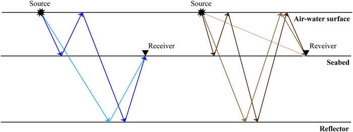
FIGURE 1. Illustrations of OBN up-going reflections and down-going reflections denoted by the blue raypaths and the brown raypaths, respectively.

Traditional imaging algorithms using up-going primaries have limits in imaging the seabed and the illumination range. The migration using the down-going first-order multiples is developed to solve the problems mentioned above. And it is also called mirror migration (Grion et al., 2007; Dash et al., 2009; Wong et al., 2015). In mirror migration, the virtual OBN position is obtained by turning the real OBN up with the sea surface as a mirror, followed by implementing conventional migration procedures. Regardless of the conventional migration or the mirror migration, the up-going multiples and down-going high-order multiples are regarded as noise and should be suppressed before or during migration. Compared with primaries and first-order down-going multiples, higher-order multiples possess longer travel paths and sufficient smaller reflection angles, which can guarantee that imaging using multiples can supply quality results with a wider illumination range (Liu et al., 2011; Lu et al., 2015; Wong et al., 2015). To make full use of the structural information contained in multiples and further increase the illumination range, we proposed RTM using down-going multiples for OBN acquisition, in which the lower-order multiples are recognized as the secondary sources of the higher-order multiples. However, the biggest challenge of RTMM is the suppression of crosstalks (Liu et al., 2011). Further, the least-squares algorithm is introduced to suppress the crosstalk noise (Nemeth et al., 1999; Dai et al., 2012; Liu et al., 2017; He et al., 2019).

The calculation cost of the migration process is linear with the total number of shot gathers. Therefore, combining several shot gathers into a supergather can effectively reduce the calculation unit and improve the calculation efficiency. However, when migrating one supergather, the interactions between the unrelated sources wavefield and the receivers wavefield will cause serious crosstalk noise, which decreases the S/N ratio of the imaging results tremendously (Romero et al., 2000; Dai et al., 2012). For example, by combining two shot gathers into one supergather and then implementing the migration, the crosscorrelation between the source wavefield activated by the first source and the receiver wavefield generated by the unrelated second backward-penetrating receiver data will produce strong crosstalks. To mitigate the above-mentioned crosstalk noise, Romero et al. (2000) first applied the phase encoding strategies in the migration procedures and showed a variety of encoding strategies. Among the commonly used encoding strategies, the random phase encoding technology Schuster et al. (2011), combining random time delays and random polarity reversals, has a better crosstalk suppression effect because it can shift and discrete crosstalk noise randomly. Krebs et al. (2009) introduced the random phase encoding scheme into the full waveform inversion and obtained results of the same quality as conventional methods, while the amount of calculation is reduced by an order of magnitude. The multi-source least-squares reverse time migration (LSRTM) proposed by Dai et al. (2012) is even more efficient than RTM, although there are some random artifacts in the imaging results. It is worth noting that to avoid convergence problems caused by the incomplete matching between the predicted data and observed data, the application of random phase encoding is generally limited to the fixed-spread acquisition geometries (Krebs et al., 2009; Dai et al., 2012; Liu et al., 2018). In the RTM of OBN down-going multiples, the lower-order multiples are recognized as the sources of the higher-order multiples, and the lower- and higher-order multiples share the same receivers. Therefore, the random phase encoding scheme can be introduced into the migration of multiples for OBN acquisition conveniently. To save the computational cost, we developed a phase-encoding-based LSRTM of OBN down-going multiples.

In this paper, we first specify the principle of RTM using OBN down-going multiples and then introduce least-squares technology to suppress crosstalks, followed by the explicit description of the phase-encoding-based LSRTM of OBN down-going multiples. Numerical experiments on the Marmousi model are used to verify the effectiveness and efficiency of the proposed approach, and the results demonstrate that the proposed approach can effectively suppress crosstalks, improve the imaging resolution, and save the computational cost. Finally, the discussion and conclusion are provided.

Theory

Common Receiver Domain RTM of OBN Down-Going Multiples

The seismic record in OBN acquisition consists of up-going and down-going components, which can be separated using PZ summation:

$\{\begin{array}{c}U=\left(P+\rho cZ\right)/2\\ D=\left(P-\rho cZ\right)/2\end{array}(1)$

where U and D denote the up-going and down-going records, respectively. P and Z represent the pressure recorded on the hydrophone and particle velocity recorded on the vertical geophone, respectively. $\rho$ and $c$ are the density and the acoustic velocity of water, respectively. As shown in Figure 2, the basic principle of PZ summation is that the geophone and the hydrophone data record opposite polarity for the down-going propagating wavefield. If the wavefield is propagating upward, they will record the same polarity.

FIGURE 2

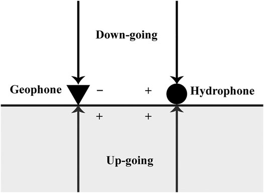
FIGURE 2. Schematic diagram of PZ summation. The hydrophone and geophone record down-going and up-going wavefield with different polarities.

In OBN acquisition, receivers are placed at the seabed sparsely, while sources are activated on the sea surface densely. For the sake of computational efficiency, the seismic reciprocal principle Knopoff and Gangi (1959) is implemented and migrations for OBN data are usually performed in the common receiver gather (CRG) domain. The data is converted from the common shot gather (CSG) into the CRG by exchanging the source and receiver locations during imaging. After conversion, the sources and nodes are regarded as the virtual receivers and the virtual sources, respectively. The conventional migration algorithms for OBN data often account for up-going primaries or down-going first-order multiples, as shown in Figures 3A,B. For the imaging of up-going primaries, the virtual sources are arranged at the seabed, which results in serious aliasing noise around the real node locations. And the subsurface coverage area of primaries is limited to the vicinity of the node positions. The mirror migration, utilizing down-going first-order multiples, can image the seabed well and enlarge the imaging range by turning the OBNs to the mirror OBNs taking the sea surface as the axis of symmetry. Both the above-mentioned migration approaches regard the up-going multiples and down-going high-order multiples as the data noise and suppress them before migration. The structural information of high-order multiples has not been fully exploited. To take full advantage of higher-order multiples, we propose RTM using down-going multiples for the OBN acquisition. Prior to the migration procedure, the down-going record is separated using PZ summation, and then the down-going multiples are acquired by muting the direct wave from the down-going record. The RTM of down-going multiples can be accomplished through the following three steps:

1 Producing the source wavefield by forward-propagating the separated down-going record including the direct wave and multiples:

$\{\begin{array}{c}\frac{1}{v_0{\left(x,z\right)}^2}\frac{{\partial }^2{P}_s\left(x,z,t\right)}{\partial t^2}={\nabla }^2{P}_s\left(x,z,t\right)\\ P_s\left(x_r,z=0,t\right)=d\left(x_r,t\right)+m\left(x_r,t\right)\end{array},(2)$

where $x_r$ is the horizontal location of virtual receivers, $v_0\left(x,z\right)$ is the migration velocity model, and $P_s\left(x,z,t\right)$ is the generated source wavefield. $d\left(x_r,t\right)$ and $m\left(x_r,t\right)$ are the direct wave and the down-going multiples in the CRG domain, respectively.

2 Backward-extrapolating the down-going multiples to obtain the receiver wavefield $M_r\left(x,z,t\right)$:

$\{\begin{array}{c}\frac{1}{v_0{\left(x,z\right)}^2}\frac{{\partial }^2{M}_r\left(x,z,t\right)}{\partial t^2}={\nabla }^2{M}_r\left(x,z,t\right)\\ M_r\left(x_r,z=0,t\right)=m\left(x_r,t\right)\end{array},(3)$

3 Implementing the zero-lag crosscorrelation imaging condition to the source and receiver wavefield:

$I\left(x,z\right)={\displaystyle \sum }_{t=0}^{t_{max}}{P}_s\left(x,z,t\right)M_r\left(x,z,t\right),(4)$

where $I\left(x,z\right)$ represents the migrated image and $t_{max}$ is the total recording time. Compared to the imaging point of mirror migration (the red solid point in Figure 3B), the imaging point of the proposed RTM using down-going multiples in Figure 3C is located at the left of that in Figure 3B (the shadow zone of mirror migration), which means wider illumination range. And theoretically with the order of multiples gets larger, the illumination can be further expanded.

FIGURE 3

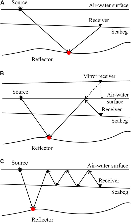
FIGURE 3. Raypath diagrams of RTM using (A) the up-going primaries (B) the down-going first-order multiples (mirror migration), and (C) all-order down-going multiples. And the red points represent the imaging points of different approaches.

Unlike conventional RTM, RTMM correlates the complex forward- and backward-penetrated records, thus the interactions among unrelated multiples will cause undesired crosstalk artifacts which critically degrade the S/N ratio of the final imaging results. Figure 4 illustrates the representative crosstalks in RTMM for OBN acquisition. In Figure 4, the red solid lines, the black solid lines, and the red dotted lines represent the wavepaths of the forward-propagating data, the backward-propagating data, and the crosscorrelation, respectively. As shown in Figure 4, the forward-propagating direct wave recorded at S3 can be regarded as the secondary source of the backward-propagating second-order multiples recorded at S1, and the crosscorrelation between the two multiples will produce crosstalk point A1 denoted by the magenta point. In Figure 4B, the crosscorrelation between the forward-propagating first-order multiples recorded at S2 and the backward-propagating first-order multiples recorded at S1 will cause the crosstalk point A2.

FIGURE 4

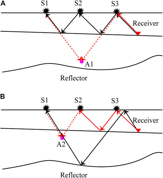
FIGURE 4. Illustrations of representative crosstalks in RTMM. As shown in panel A, the crosscorrelation between the forward-propagating direct wave recorded at S3 and the backward-propagating second-order multiples recorded at S1 will generate the crosstalk point A1 denoted by the magenta point. In panel B, the first-order multiple recorded at S2 can be regarded as the secondary source of the backward-propagating first-order multiple recorded at S3, and the crosscorrelation of the two multiples will cause crosstalk point A2.

LSRTM of OBN Down-Going Multiples

Compared with RTM, the LSRTM has been extensively researched to enhance the imaging quality by suppressing RTM imaging artifacts, improving the imaging resolution, and balancing the energies of imaging events. LSRTM also can be extended to the migration of multiples to suppress the severe crosstalks of RTMM. Unlike the conventional LSRTM using primaries, LSRTM of multiples (LSRTMM) Zhang and Schuster (2014), Wong et al. (2015), Liu X. et al. (2016) regards multiples data as the secondary source and tries to find a reflectivity model that minimizes the misfit function between predicted and observed multiple reflections. The Born modeling operator (see Appendix A) that corresponds to the multiples can be represented as

$\{\begin{array}{c}\frac{1}{v_0{\left(x,z\right)}^2}\frac{{\partial }^{2}M\left(x,z,t\right)}{\partial t^2}-{\nabla }^{2}M\left(x,z,t\right)=d\left(x_r,t\right)+m\left(x_r,t\right)\\ \frac{1}{v_0{\left(x,z\right)}^2}\frac{{\partial }^2{M}_r\left(x,z,t\right)}{\partial t^2}-{\nabla }^2{M}_r\left(x,z,t\right)=-R(x,z)\frac{{\partial }^{2}M\left(x,z,t\right)}{\partial t^2}\\ m_{pre}\left(x_r,t\right)=M_r\left(x_r,z=0,t\right)\end{array}.(5)$

Eq. (5) contains three steps: 1) The down-going record of OBN data $d\left(x_r,t\right)+m\left(x_r,t\right)$ are treated as the virtual sources and injected into the subsurface background model $v_0$, which will produce the incident wavefield $M$. 2) The interaction between the incident wavefield $M$ and the subsurface reflectivity $R$ will generate the scattered wavefield $M_r$. 3) Through saving the boundary wavefield of the scattered wavefield $M_r$, we can obtain the predicted down-going multiples $m_{pre}$. Eq. (5) can be depicted compactly using a matrix-vector notation:

$m_{pre,i}=L_{i}R(6)$

where $L_i$ and $m_{pre,i}$ represent the linear Born modeling operator and the predicted OBN down-going multiples for the ith CRG, respectively. The RTM operator can be treated as the adjoint of the forward-modeling operator, thus the final migrated image $R_{mig}$ can be obtained by:

$R_{mig}=\left[L_1^T{L}_2^T\cdots L_n^T\right]\left[\begin{array}{c}\begin{array}{c}{m}_1\\ m_2\\ ⋮\end{array}\\ m_n\end{array}\right]={\displaystyle \sum }_{i=0}^n{L}_i^T{m}_i(7)$

where the superscript $T$ is the conjugate transpose operation. $L_i^T$ and $m_i$are the migration operator and the observed down-going multiples for the ith CRG, respectively.

Based on the Born modeling operator defined in Eq. 5 and its adjoint RTM operator in Eq. (7), we can minimize the difference between the modeled/predicted multiples and the observed multiples via the misfit function $f\left(R\right)$,

$f\left(R\right)=\frac{1}{2}{\displaystyle \sum }_{i=0}^n\Vert L_{i}R-m_i{\Vert }_2^2(8)$

which can be iteratively solved aided by any gradient-based inversion approach.

LSRTM of OBN Down-Going Multiples With Random Phase Encoding

However, in LSRTM, each iteration contains migration, de-migration and gradient calculation steps, the calculation cost of which is several times of that of RTM. And the computational cost of LSRTM for OBN down-going multiples may be larger for more iterations are needed to achieve better crosstalk artifacts suppression effect. Therefore, we introduce the random phase encoding scheme into LSRTM of OBN down-going multiples to improve the computational efficiency. By encoding the forward modeling operators (in Eq. (6)), OBN down-going multiples of different CRGs can be simultaneously modeled as

$\left[{\alpha }_1+{\alpha }_2+\cdots +{\alpha }_n\right]m_{pre,i}=\left[{\alpha }_1{L}_1+{\alpha }_2{L}_2+\cdots +{\alpha }_n{L}_n\right]R(9)$

where ${\alpha }_n$ is the phase encoding function. Eq. (9) can be written in a compact form of

${\check{m}}_{pre}=\check{L}R(10)$

where $\check{L}$ and ${\check{m}}_{pre}$ represent the encoded forward modeling operator and predicted data for one supergather, respectively. The image of a supergather of observed OBN down-going multiples $\check{m}$ can be produced by

${\check{R}}_{mig}={\check{L}}^T\check{m}(11)$

where ${\check{R}}_{mig}$ represents the phase-encoded image of OBN down-going multiples. Eq. (12) is the expanded form of Eq. (11)

${\check{R}}_{mig}=\left[{\alpha }_1^{\ast }{L}_1^T+{\alpha }_2^{\ast }{L}_2^T+\cdots +{\alpha }_n^{\ast }{L}_n^T\right]\times \left[{\alpha }_1\check{m_1}+{\alpha }_2\check{m_n}+\cdots +{\alpha }_n\check{m_n}\right]$

$={\displaystyle \sum }_{i=1}^n{\alpha }_i^{\ast }{\alpha }_i{L}_i^T\check{m_i}+{\displaystyle \sum }_{i=1}^n{\displaystyle \sum }_{j\ne i}^n{\alpha }_i^{\ast }{\alpha }_j{L}_i^T\check{m_i}$

$=\underset{valid term}{\underbrace{{\displaystyle \sum }_{i=1}^n{L}_i^T\check{m_i}}}+\underset{noise term}{\underbrace{{\displaystyle \sum }_{i=1}^n{\displaystyle \sum }_{j\ne i}^n{\alpha }_i^{\ast }{\alpha }_j{L}_i^T\check{m_i}}}(12)$

where for any integer value i, we assume that ${\alpha }_i^{\ast }{\alpha }_i=1$. In Eq. (12), the valid term, which is identical with Eq. (7), will produce the correct imaging result and crosstalks. The noise term only generates crosstalk noise, which is caused by the interaction between the encoded CRGs. For phase-encoding-based RTM of OBN down-going multiples, the crosstalk noise generated by the noise term is much stronger than the noise generated by the valid term (Liu et al., 2018). In the numerical experiment section, we will illustrate the different crosstalks caused by the valid and noise terms of Eq. (12). Through encoding ns supergathers from original CRGs and based on Eqs (10) and (11), the objective function of phase-encoding-based LSRTM of OBN down-going multiples is expressed as

$f\left(R\right)=\frac{1}{2}{\displaystyle \sum }_{i=1}^{ns}\Vert \check{L}R-{\check{m}}_i{\Vert }_2^2(13)$

The implementation details of the proposed migration approach are illustrated in Figure 5. One of the key steps to the proposed approach is the choice of the phase encoding functions. In this paper, the phase encoding function is designed as

${\alpha }_n=e^{-iw{\tau }_n}{S}_n(14)$

where ${\tau }_n$ and $S_n$ denote the random time delay and random polarity reversal for a blended CRG, respectively. The random time delays ${\tau }_n$ follows the normal distribution with a standard deviation of $\sigma$ and a mean of zero, expressed as:

${\tau }_n\sim N\left(0,{\sigma }^2\right).(15)$

FIGURE 5

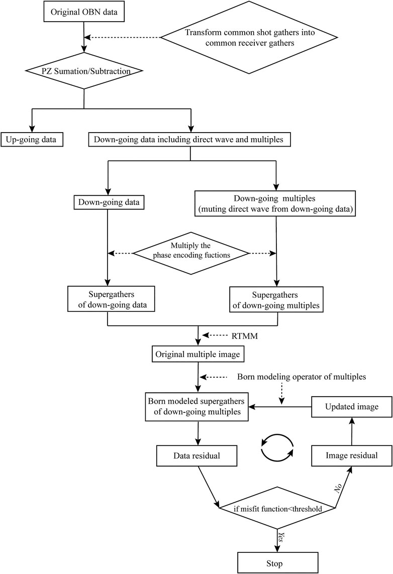
FIGURE 5. The workflow of the fast LSRTM using down-going multiples.

The probability that the polarity reversal function $S_n$ takes a value of 1 or -1 for each blended CRG is 1/2. According to the property of normal distribution, the polarity reversal function $S_n$ can be defined by the following:

$S_n=sgn\left({\tau }_n\right),(16)$

where $sgn$ represents the sign function. If ${\tau }_n\ge 0 S_n=1$, otherwise $S_n=-1$.

Numerical Examples

In this section, we apply the proposed phase-encoding-based LSRTM of OBN down-going multiples on the Marmousi model. A high-order staggered-grid finite-difference algorithm with PML absorbing boundaries is utilized to solve the first-order velocity-stress acoustic wave equations and produce the OBN data. The results of conventional RTM using primaries and mirror migration are also used to verify the effectiveness of the proposed approach.

The Behavior of Conventional LSRTM of OBN Down-Going Multiples

Figure 6 shows the Marmousi velocity model. The model is discretized into 351 grids in the vertical direction and 1,001 grids in the horizontal direction both with a 10 m grid interval. The seismic source is selected as the Ricker wavelet with a peak frequency of 20 Hz. A set of 1,001 CSGs with a source interval of 10 m are simulated to certify the performance of the novel approach. The total recording time of each CSG is 4s with a sampling interval of 4 m s. First, we make use of 20 OBNs, distributed evenly from 2.98 to 6.78 km in the horizontal direction with a 200-m node interval, to test the imaging performances of RTM and LSRTM of down-going multiples. The pressure components of a CSG and a converted CRG are illustrated in Figure 7A,B respectively. The up-going and down-going records after PZ summation are displayed in Figure 8A,B, respectively. The down-going multiples after muting the direct wave from the down-going record (Figure 8) are shown in Figure 8C.

FIGURE 6

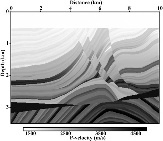
FIGURE 6. The Marmousi velocity model.

FIGURE 7

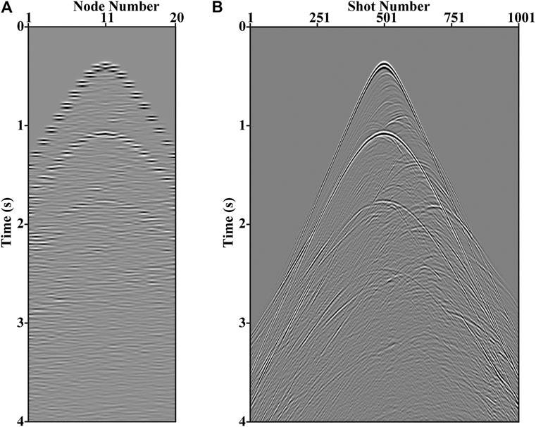
FIGURE 7. The hydrophone pressures of (A) a CSG and (B) a converted CRG with a node interval.

FIGURE 8

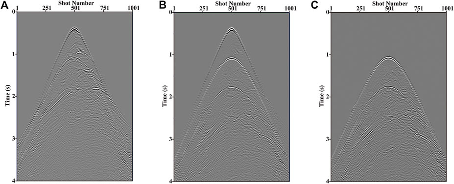
FIGURE 8. The CRGs of (A) the up-going and (B) down-going pressures obtained after applying PZ summation (C) the down-going multiples acquired by muting direct wave from panel B.

In the CRG domain, since the seismometers are placed at the seabed and they act as the virtual sources, there is strong aliasing noise around the seabed in the image of the conventional RTM using up-going primaries as shown by the arrow in Figure 9A. Moreover, the illumination range of Figure 9A is limited to the vicinity of the node positions due to the insufficient subsurface coverage of up-going primaries. To settle the above-mentioned problems, the RTM using the down-going first-order multiples (mirror migration) is developed. As shown in Figure 9B, the imaging quality of the seabed has been greatly improved pointed out by the arrow, and the illumination range has also been expanded compared with the imaging result of up-going primaries in Figure 9A. To make full advantage of higher-order multiples, the proposed RTM of OBN down-going multiples algorithm is implemented, and the imaging result is displayed in Figure 9C. Compared with the results in Figures 9A,B, the imaging result of all-order multiples in Figure 9C shows a much wider illumination range. However, the interferences among unrelated multiples cause crosstalk artifacts which degrade the imaging fidelity as denoted by the arrows in Figure 9C. The kind of crosstalks is inherent in conventional RTMM results (Eq. (7) or the valid term of Eq. (12)) (Liu et al., 2011). Compared with RTM of down-going multiples, the developed LSRTM of down-going multiples can suppress the crosstalks effectively as pointed out by the arrows in Figures 9C,D, and produce a higher-resolution image (Figure 9D).

FIGURE 9

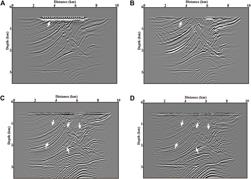
FIGURE 9. Migration results of (A) up-going primaries (B) down-going first-order multiples, and down-going all-order multiples (C) with and (D) without least-squares algorithm (10 iterations) with a node interval of 100 m. The arrows in panels C and D denote the inherent crosstalks which can be suppressed effectively by LSRTMM.

The Behavior of the Proposed Phase-Encoding-Based LSRTM of OBN Down-Going Multiples

Subsequently, the node interval is reduced from 200 to 100 m, and a total of 40 nodes are evenly placed at the seabed from 2.98 to 6.88 km. After the simulation and PZ summation, 40 CRGs are encoded into 1, 2, 4, 8, 20 supergathers to verify the effectiveness and efficiency of the proposed phased-encoding-based algorithm. The random encoding function which combines the random time delays and polarity reversals is utilized to blend different CRGs. The random time delay sequences distribute normally with a 0.5 standard deviation and zero mean. The blended supergathers of 1, 2, 5,10, 20, and 40 CRGs of down-going multiples are illustrated in Figure 10, respectively. Images generated by RTM of up-going primaries, down-going first-order multiples (mirror migration), and down-going multiples are shown in Figures 11A–C, respectively. Figure 11D represents the result of LSRTM of down-going multiples. Compared with the images with the 200 m node interval in Figure 9, the corresponding images with the 100 m node interval provide more sufficient subsurface coverage, more continuous strata, and a higher S/N ratio.

FIGURE 10

FIGURE 10. The blended supergathers by encoding (A) 1 (B) 2 (C) 5 (D) 10 (E) 20, and (F) 40 CRGs of down-going multiples with a node interval of 100 m.

FIGURE 11

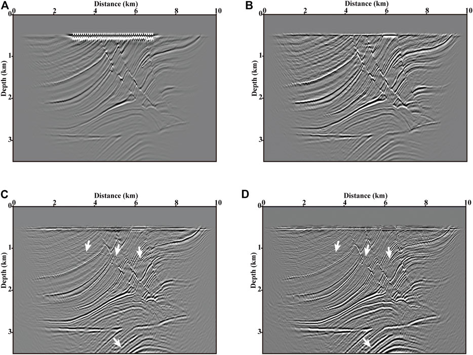
FIGURE 11. Migration images of (A) up-going primaries (B) down-going first-order multiples, and down-going all-order multiples (C) with and (D) without least-squares algorithm (10 iterations) with a node interval of 100 m. As denoted by the arrows in panels C and D, the LSRTM can improve the imaging quality effectively.

In the following, we use five sets of supergathers that regard the number of encoding CRGs as the variable to present the effectivity and efficiency of the proposed phase-encoding-based LSRTM of down-going multiples. Figures 12–16 display the RTM and LSRTM (10 iterations) images using the supergathers in Figures 10B–F, respectively. Compared with the RTM, the LSRTM can effectively suppress the noise caused by the interferences among encoded CRGs (the noise term of Eq. 12) and significantly improve the imaging resolution as shown by the arrows in panels A and B of Figures 12–16. From the five pairs of migration results, as the number of encoding CRGs decreases, the imaging results are getting closer to those of conventional migrations (Figures 11C,D). The trend is caused by the decrease of the energy proportion of the noise term in Eq. (12). However, as the number of encoding CRGs decreases, the computational cost will increase. In the last two experiments, the original 40 shot gathers are encoded into 8 and 20 supergathers, respectively. And the final results (Figures 15, 16) show better imaging qualities and a higher S/N ratio compared with those results in Figures 12–14. Therefore, we choose them to conduct the calculation comparison with conventional LSRTM of down-going multiples. Scaling all calculations to the forward modeling, each iteration of the LSRTM requires 6 forward modelings including two for the RTM, two for the de-migration, and two for the gradient calculation. The conventional LSRTM of down-going multiples with 40 supergathers and 10 iterations (see Figure 11D) requires a computational cost of 40 × 6 × 10 = 2,400 forward modelings. The computational costs for LSRTM images in Figure 15B (8 supergathers) and Figure 16B (20 supergathers) are 8 × 6 × 10 = 480 and 20 × 6 × 10 = 1,200 forward modelings, respectively. The comparison of computational cost demonstrates that the proposed phased-encoded LSRTM method can provide the results which can meet the requirement of interpretation and improve the computational efficiency manyfold.

FIGURE 12

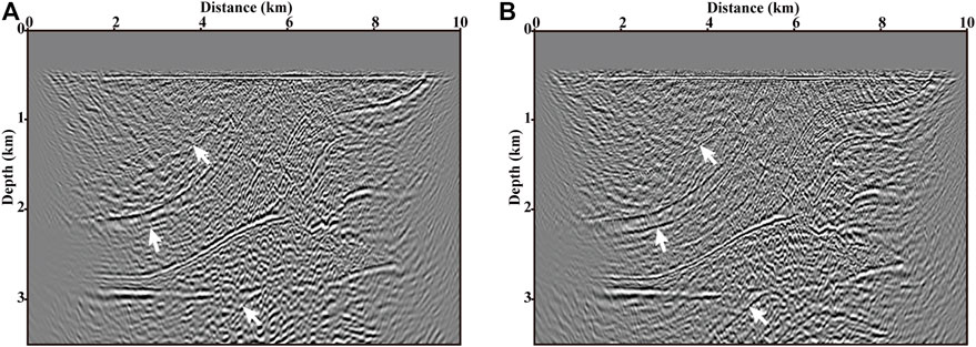
FIGURE 12. Images provided by (A) RTM and (B) LSRTM of one blended supergather of 40 CRGs after 10 iterations.

FIGURE 13

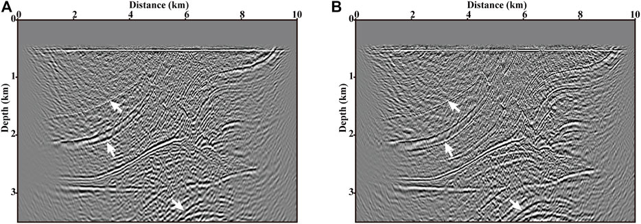
FIGURE 13. Images provided by (A) RTM and (B) LSRTM of two blended supergathers of 20 CRGs after 10 iterations.

FIGURE 14

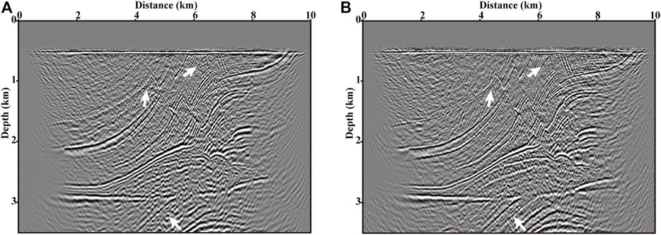
FIGURE 14. Images provided by (A) RTM and (B) LSRTM of four blended supergathers of 10 CRGs after 10 iterations.

FIGURE 15

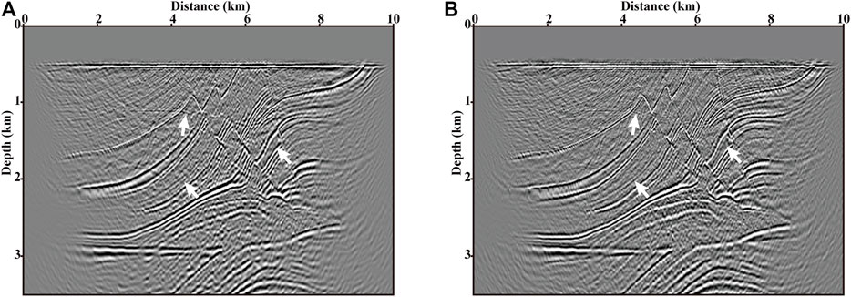
FIGURE 15. Images provided by (A) RTM and (B) LSRTM of eight blended supergathers of 5 CRGs after 10 iterations.

FIGURE 16

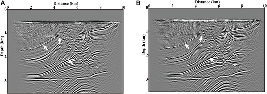
FIGURE 16. Images provided by (A) RTM and (B) LSRTM of twenty blended supergathers of two CRGs after 10 iterations.

Discussion

Up to now, there are two widely used crosstalk suppression methods in the migration of multiples. The first one is the LSRTMM which introduces least-squares optimal algorithms to suppress crosstalks and obtains higher-precision images of multiples migration. The second one is the RTM of controlled-order multiples (RTM-CM) in which the different orders of multiples are extracted before migration procedures and the separated nth-order and (n+1)th-order multiples respectively act as the source and receiver data. RTM-CM can significantly reduce the crosstalks due to the simplifies of the forward- and backward-propagating data. Liu Y. et al. (2016) separated different orders of multiples using surface-related multiple elimination (SRME) and then proposed LSRTM-CM. Compared with LSRTMM, LSRTM-CM obtains images with a higher S/N ratio. When extracting multiples of different orders by conventional SRME, the locations of sources and receivers must keep coincident. However, in OBN acquisition, shots are activated densely on the sea surface and seismometers are sparsely placed at the seabed, which makes it difficult to isolate different-order up- or down-going multiples. Therefore, in this study, LSRTMM is utilized to suppress crosstalks rather than RTM-CM. The least-squares algorithms can not only suppress the inherent crosstalks of multiple imaging but also reduce the noises caused by interactions among the encoding CRGs.

In this paper, we select the static phase encoding strategy, that is, during the entire least squares implementation the encoding function remains constant, which will result in the undesired suppression of the crosstalk noise generated by the encoded CRGs. In the following research, we will design an optimal dynamic phase encoding scheme to achieve a better noise suppression effect. It should be illustrated that we assumed that the geophones and the hydrophones are placed above the seabed. Consequently, the acquired synthetic data only contain P-wave components. And the pressure component P and the particle velocity component Z directly can be obtained directly by using the first-order velocity-stress acoustic wave equation. S-wave information is the key to the data processing of OBN acquisition, and the availability and efficiency of the proposed method on S-wave remain to be verified. In the following researches, we will concentrate on the exploitation of S-wave information.

Conclusion

Conventional imaging approaches of OBN data account for the up-going primaries and the down-going first-order multiples. However, OBN data contain the up-going multiples and down-going higher-order multiples, and the information carried by those multiples could also be used to enhance the imaging quality. In this paper, we developed a CRG-domain LSRTM of OBN down-going multiples with a random phase encoding scheme in which the full down-going data and down-going multiples are recognized as secondary sources and observed data. The encoding function is composed of random time delay sequences and random polarity reversals which are designed as a normal distribution. Synthetic experiments demonstrate that the proposed approach can efficiently produce images with a wide illumination range and high resolution. Our approach has the potential to serve as a powerful tool for imaging OBN data of complex subsurface structures.

Data Availability Statement

The original contributions presented in the study are included in the article/Supplementary Material, further inquiries can be directed to the corresponding author.

Author Contributions

YZ and YL contributed as the major authors of the manuscript. JY did a part of writing and coding works. XL provided some constructive ideas and polished the manuscript. All authors contributed to the article and improved the submitted version.

Funding

The research was partially funded by the National Nature Science Foundation of China (Grant No. 41730425), the Special Fund of the Institute of Geophysics, China Earthquake Administration (Grant No. DQJB20K42), and the Institute of Geology and Geophysics, Chinese Academy of Sciences Project (Grant No. IGGCAS-2019031).

Conflict of Interest

The authors declare that the research was conducted in the absence of any commercial or financial relationships that could be construed as a potential conflict of interest.

Publisher’s Note

All claims expressed in this article are solely those of the authors and do not necessarily represent those of their affiliated organizations, or those of the publisher, the editors and the reviewers. Any product that may be evaluated in this article, or claim that may be made by its manufacturer, is not guaranteed or endorsed by the publisher.

References

Alerini, M., Traub, B., Ravaut, C., and Duveneck, E. (2009). Prestack Depth Imaging of Ocean-Bottom Node Data. Geophysics 74 (6), WCA57–WCA63. doi:10.1190/1.3204767

CrossRef Full Text | Google Scholar

Barr, F. J., and Sanders, J. I. (1989). Attenuation of Water‐column Reverberations Using Pressure and Velocity Detectors in a Water‐bottom cable. 59th Annu. Int. Meet. SEG, Expanded Abstr. 8, 653–655. doi:10.1190/1.1889557

CrossRef Full Text | Google Scholar

Berkhout, A. J., and Verschuur, D. J. (2006). Imaging of Multiple Reflections. Geophysics 71 (4), SI209–SI220. doi:10.1190/1.2215359

CrossRef Full Text | Google Scholar

Dai, W., Fowler, P., and Schuster, G. T. (2012). Multi-source Least-Squares Reverse Time Migration. Geophys. Prospect. 60, 681–695. doi:10.1111/j.1365-2478.2012.01092.x

CrossRef Full Text | Google Scholar

Dash, R., Spence, G., Hyndman, R., Grion, S., Wang, Y., and Ronen, S. (2009). Wide-area Imaging from OBS Multiples. Geophysics 74, Q41–Q47. doi:10.1190/1.3223623

CrossRef Full Text | Google Scholar

Dragoset, B., Verschuur, E., Moore, I., and Bisley, R. (2010). A Perspective on 3D Surface-Related Multiple Elimination. Geophysics 75 (5), 75A245–75A261. doi:10.1190/1.3475413

CrossRef Full Text | Google Scholar

Grion, S., Exley, R., Manin, M., Miao, X., Pica, A. L., Wang, Y., et al. (2007). Mirror Imaging of OBS Data. First Break 25, 37–42. doi:10.3997/1365-2397.2007028

CrossRef Full Text | Google Scholar

He, B., Liu, Y., and Zhang, Y. (2019). Improving the Least-Squares Image by Using Angle Information to Avoid Cycle Skipping. Geophysics 84 (6), S581–S598. doi:10.1190/geo2018-0816.1

CrossRef Full Text | Google Scholar

Jiang, Z., Sheng, J., Yu, J., Schuster, G. T., and Hornby, B. E. (2007). Migration Methods for Imaging Different-Order Multiples. Geophys. Prospect. 55, 1–19. doi:10.1111/j.1365-2478.2006.00598.x

CrossRef Full Text | Google Scholar

Katzman, R., Holbrook, W. S., and Paull, C. K. (1994). Combined Vertical-Incidence and Wide-Angle Seismic Study of a Gas Hydrate Zone, Blake Ridge. J. Geophys. Res. 99 (B9), 17975–17995. doi:10.1029/94JB00662

CrossRef Full Text | Google Scholar

Knopoff, L., and Gangi, A. F. (1959). Seismic Reciprocity. Geophysics 24, 681–691. doi:10.1190/1.1438647

CrossRef Full Text | Google Scholar

Krebs, J. R., Anderson, J. E., Hinkley, D., Neelamani, R., Lee, S., Baumstein, A., et al. (2009). Fast Full-Wavefield Seismic Inversion Using Encoded Sources. Geophysics 74 (6), WCC177–WCC188. doi:10.1190/1.3230502

CrossRef Full Text | Google Scholar

Li, Z., Li, Z., Wang, P., and Zhang, M. (2017). Reverse Time Migration of Multiples Based on Different-Order Multiple Separation. Geophysics 82 (1), S19–S29. doi:10.1190/geo2015-0710.1

CrossRef Full Text | Google Scholar

Liu, X., Liu, Y., Hu, H., Li, P., and Khan, M. (2016a). Imaging of First-Order Surface-Related Multiples by Reverse-Time Migration. Geophys. J. Int. 208 (2), 1077–1087. doi:10.1093/gji/ggw437

CrossRef Full Text | Google Scholar

Liu, X., Liu, Y., and Khan, M. (2018). Fast Least-Squares Reverse Time Migration of VSP Free-Surface Multiples with Dynamic Phase-Encoding Schemes. Geophysics 83 (4), S321–S332. doi:10.1190/geo2017-0419.1

CrossRef Full Text | Google Scholar

Liu, X., Liu, Y., Lu, H., Hu, H., and Khan, M. (2017). Prestack Correlative Least-Squares Reverse Time Migration. Geophysics 82 (2), S159–S172. doi:10.1190/geo2016-0416.1

CrossRef Full Text | Google Scholar

Liu, X., and Liu, Y. (2018). Plane-wave Domain Least-Squares Reverse Time Migration with Free-Surface Multiples. Geophysics 83 (6), S477–S487. doi:10.1190/geo2017-0570.1

CrossRef Full Text | Google Scholar

Liu, Y., Chang, X., Jin, D., He, R., Sun, H., and Zheng, Y. (2011). Reverse Time Migration of Multiples for Subsalt Imaging. Geophysics 76 (5), WB209–WB216. doi:10.1190/geo2010-0312.1

CrossRef Full Text | Google Scholar

Liu, Y., Hu, H., Xie, X.-B., Zheng, Y., and Li, P. (2015). Reverse Time Migration of Internal Multiples for Subsalt Imaging. Geophysics 80, S175–S185. doi:10.1190/geo2014-0429.1

CrossRef Full Text | Google Scholar

Liu, Y., Jin, D., Chang, X., Li, P., Sun, H., and Luo, Y. (2010). Multiple Subtraction Using Statistically Estimated Inverse Wavelets. Geophysics 75 (6), WB247–WB254. doi:10.1190/1.325549910.1190/1.3494082

CrossRef Full Text | Google Scholar

Liu, Y., Liu, X., Osen, A., Shao, Y., Hu, H., and Zheng, Y. (2016b). Least-squares Reverse Time Migration Using Controlled-Order Multiple Reflections. Geophysics 81 (5), S347–S357. doi:10.1190/geo2015-0479.1

CrossRef Full Text | Google Scholar

Lu, S., Whitmore, D. N., Valenciano, A. A., and Chemingui, N. (2015). Separated-wavefield Imaging Using Primary and Multiple Energy. The Leading Edge 34, 770–778. doi:10.1190/tle34070770.1

CrossRef Full Text | Google Scholar

Muijs, R., Robertsson, J. O., and Holliger, K. (2007). Prestack Depth Migration of Primary and Surface-Related Multiple Reflections: Part I - Imaging. Geophysics 72 (2), S59–S69. doi:10.1190/1.2422796

CrossRef Full Text | Google Scholar

Nemeth, T., Wu, C., and Schuster, G. T. (1999). Least‐squares Migration of Incomplete Reflection Data. Geophysics 64, 208–221. doi:10.1190/1.1444517

CrossRef Full Text | Google Scholar

Romero, L. A., Ghiglia, D. C., Ober, C. C., and Morton, S. A. (2000). Phase Encoding of Shot Records in Prestack Migration. Geophysics 65, 426–436. doi:10.1190/1.1444737

CrossRef Full Text | Google Scholar

Schalkwijk, K. M., Wapenaar, C. P. A., and Verschuur, D. J. (2003). Adaptive Decomposition of Multicomponent Ocean‐bottom Seismic Data into Downgoing and Upgoing P‐ and S‐waves. Geophysics 68, 1091–1102. doi:10.1190/1.1581081

CrossRef Full Text | Google Scholar

Schuster, G. T., Wang, X., Huang, Y., Dai, W., and Boonyasiriwat, C. (2011). Theory of Multisource Crosstalk Reduction by Phase-Encoded Statics. Geophys. J. Int. 184, 1289–1303. doi:10.1111/j.1365-246X.2010.04906.x

CrossRef Full Text | Google Scholar

Verschuur, D. J., and Berkhout, A. J. (2011). Seismic Migration of Blended Shot Records with Surface-Related Multiple Scattering. Geophysics 76 (1), A7–A13. doi:10.1190/1.3521658

CrossRef Full Text | Google Scholar

Verschuur, D. J., Berkhout, A. J., and Wapenaar, C. P. A. (1992). Adaptive Surface‐related Multiple Elimination. Geophysics 57, 1166–1177. doi:10.1190/1.1443330

CrossRef Full Text | Google Scholar

Wong, M., Biondi, B. L., and Ronen, S. (2015). Imaging with Primaries and Free-Surface Multiples by Joint Least-Squares Reverse Time Migration. Geophysics 80 (6), S223–S235. doi:10.1190/geo2015-0093.1

CrossRef Full Text | Google Scholar

Zhang, D., and Schuster, G. T. (2014). Least-squares Reverse Time Migration of Multiples. Geophysics 79 (1), S11–S21. doi:10.1190/geo2015-0479.110.1190/geo2013-0156.1

CrossRef Full Text | Google Scholar

Zhang, Y., Liu, Y., and Liu, X. (2019). Reverse Time Migration Using Controlled-Order Water-Bottom-Related Multiples. 89th Annu. Int. Meet. SEG, Expanded Abstr., 4261–4265. doi:10.1190/segam2019-3206145.1

CrossRef Full Text | Google Scholar

Zhang, Y., Liu, Y., Liu, X., and Zhou, X. (2020). Reverse Time Migration Using Water‐bottom‐related Multiples. Geophys. Prospecting 68 (2), 446–465. doi:10.1111/1365-2478.12851

CrossRef Full Text | Google Scholar

Zuberi, A., and Alkhalifah, T. (2013). Imaging by Forward Propagating the Data: Theory and Application. Geophys. Prospect. 61, 248–267. doi:10.1111/1365-2478.12006

CrossRef Full Text | Google Scholar

Appendix A: Born modeling for OBN down-going data

The LSRTM is generally utilized to enhance the quality of an image $R$ by minimizing the difference between the observed data $d_{obs}\left(x_r,t\right)$ and the predicted data $d_{pre}\left(x_r,t\right)$ via the following misfit function:

$f\left(R\right)=\frac{1}{2}{\displaystyle \sum }_{i=0}^n\Vert d_{obs}\left(x_r,t\right)-d_{pre}{\left(x_r,t\right)\Vert }_2^2.(\mathrm{A1})$

The acoustic wave equation in the time $t$ and space $\left(x,z\right)$ domain is provided in a reference medium as

$\frac{1}{v_0{\left(x,z\right)}^2}\frac{{\partial }^2{P}_0\left(x,z,t\right)}{\partial t^2}-{\nabla }^2{P}_0\left(x,z,t\right)=\delta \left(x-x_s,z-z_s\right)S\left(t\right)(\mathrm{A2})$

where $v_0\left(x,z\right)$represents the acoustic wave propagation velocity in the background/reference medium, $P_0\left(x,z,t\right)$ denotes the pressure wavefield. $\left(x_s,z_s\right)$ is the location of a source, and $S\left(t\right)$ indicates the source function. The perturbation method is used to explain the wavefield $P\left(x,z,t\right)$ in the real medium $v(x,z)$. A velocity perturbation $\delta v\left(x,z\right)=v-v_0$ between the real and background medium can cause a wavefield perturbation$\mathit{ \delta P}\left(\mathit{x},\mathit{z},\mathit{t}\right)=\mathit{P}-{\mathit{P}}_0$, which can be estimated by Born modeling:

$\frac{1}{v_0{\left(x,z\right)}^2}\frac{{\partial }^2\delta P\left(x,z,t\right)}{\partial t^2}-{\nabla }^2\delta P\left(x,z,t\right)\approx R\left(x,z\right)\frac{{\partial }^2{P}_0\left(x,z,t\right)}{\partial t^2}.(\mathrm{A3})$

where $R\left(x,z\right)=-2\delta v\left(x,z\right)/v_0{\left(x,z\right)}^3$ is the reflectivity model which is corresponding to the velocity perturbation$\delta v\left(x,z\right)$. The wavefield perturbation $\delta P\left(x,z,t\right)$ can be obtained by solving Eqs A2 and A3, and then the predicted data can be acquired by $d_{pre}\left(x_r,t\right)=\delta P\left(x_r,0,t\right)$.

In imaging with multiples, the lower-order multiples can be recognized as the virtual secondary source, and then they are forward extrapolated into the earth to produce higher-order multiples. Consequently, for OBN down-going multiples, we adjust Eq. A2 by incorporating direct wave$d\left(x_r,t\right)$ and down-going multiples$m\left(x_r,t\right)$ in the right side of the equation and combine it with Eq. A3. The Born modeling operator associated with the OBN down-going data is thus given by:

$\{\begin{array}{c}\frac{1}{v_0{\left(x,z\right)}^2}\frac{{\partial }^{2}M\left(x,z,t\right)}{\partial t^2}-{\nabla }^{2}M\left(x,z,t\right)=d\left(x_r,t\right)+m\left(x_r,t\right)\\ \frac{1}{v_0{\left(x,z\right)}^2}\frac{{\partial }^2{M}_r\left(x,z,t\right)}{\partial t^2}-{\nabla }^2{M}_r\left(x,z,t\right)=-R(x,z)\frac{{\partial }^{2}M\left(x,z,t\right),}{\partial t^2}\\ m_{pre}\left(x_r,t\right)=M_r\left(x_r,z=0,t\right)\end{array}(\mathrm{A4})$

where $m_{pre}\left(x_r,t\right)$ denotes the predicted down-going multiples. $M$ and $M_r$ represents the background and perturbation wavefields, respectively.