Long-Term Spatial and Temporal Variation of Near Surface Air Temperature in Southwest China During 1969–2018

Introduction

Near surface air temperature (NSAT) is a key meteorological parameter involved in exchanges of energy and water in land-atmosphere interactions. It is also a key atmospheric variable with direct influence on physical and biological processes, including energy and water balances, nutrient cycling, growth and yield, carbon dynamics, and ecosystem adaption (Joly et al., 2011; Wang et al., 2017; Cui and Shi, 2021). NSAT is typically measured at a height of 2.0 m above the ground with high precision and high temporal resolution, through irregularly distributed meteorological stations (Wang et al., 2017). Understanding about the spatial-temporal variability of NSAT is required in hydrology, meteorology, and ecology (Peng et al., 2019). Thus, it is important to assess how climate change has altered the NSAT in spatial and temporal terms, and to enhance our understanding of its variability. However, this is often limited by the spatial coverage of instrumental records, especially in regions where meteorological stations are insufficient and distributed unevenly in space (Ilori and Ajayi, 2020).

A typical way to fill in this gap is by adopting the interpolation method, which estimates plausible values based on the discrete known values (Nalder and Wein, 1998). As a result, interpolation is commonly applied to estimate the spatial distribution of NSAT for regional scales (Fick and Hijmans, 2017). However, it is known that no single interpolation method is optimal for all regions, and the performance of an interpolating method is strongly affected by many factors, e.g., sample distribution and density, surface type, data variance, data normality, grid resolution, as well as the interactions among these factors (Li and Heap, 2011). Consequently, there has been growing interest in the development of methods for interpolating in-situ gauged data from sparse networks (Khosravi and Balyani, 2019). So far, a number of interpolation methods have been developed to obtain spatially continuous NSAT from point station measurements, including inverse distance weighting, regression analysis, kriging, and spline methods (Wu and Li, 2013; Kayikci and Kazanci, 2016; Hadi and Tombul, 2018; Jiang et al., 2019; Collados-Lara et al., 2021).

Many studies have evaluated the spatial-temporal variations of NSAT around the globe. In general, they reported the consistent and significant increase in NSAT over the past 100 years (Ding et al., 2007; Ren et al., 2016; Luo and Lau, 2017; Amato et al., 2019; Zhou et al., 2020). For example, the global average NSAT was trending upward at 0.145°C/decade in 1951–2019 (Li et al., 2021). In China, the NSAT was increasing at 0.150°C/decade in 1959–2014 (Cui et al., 2017). Moreover, there was a hiatus or slowdown in the warming period following the 1997/1998 EL Niño event at both global and regional scales (Easterling and Wehner, 2009; Cahill et al., 2015; Fyfe et al., 2016; Sun et al., 2018; Lewandowsky et al., 2018; Risbey et al., 2018; Li et al., 2021). For China, some studies have also indicated about a slowdown in the warming trend since 1998 (Tang et al., 2012; Li et al., 2015), which is more pronounced than the global mean (Du et al., 2019).

The challenge of estimating NSAT is primarily in mountainous or high elevation areas, where instrumental records are not always available due to the paucity of weather stations (Wang et al., 2017; Collados-Lara et al., 2021). Earlier studies have demonstrated that co-kriging and ANUSPLIN (abbreviation for Australian National University Spline) are more suitable for sparse data in these regions (Hutchinson and Gessler, 1994; Price et al., 2000; Islam and Déry, 2017; Mohammadi et al., 2017; Zhao et al., 2019; Belkhiri et al., 2020; Cheng et al., 2020; Guo et al., 2020). An advantage of these two interpolation methods is that they can model the terrain effect by considering additional variables during interpolation process (Cuervo-Robayo et al., 2014). Nevertheless, in most cases, both co-kriging and ANUSPLIN would ignore some important terrain-related factors (such as slope and aspect), which could influence the amount of Sun radiation on land surface and then affect NSAT (Minder et al., 2010; Zhao et al., 2019; Persaud et al., 2020). Thus, it is reasonable to refine the interpolation results of NSAT by incorporating more terrain-related variables, especially in topographically heterogeneous regions (Price et al., 2000).

It was reported that mountainous areas are especially sensitive and vulnerable to climate change (Diaz and Bradley, 1997). Even relatively small climate changes could have major implications for animal, plant, and people living in these regions (Fan et al., 2011). Hence, man studies have been conducted to understand the associated impacts of climate change in mountainous regions (Lin et al., 2017; Li et al., 2020). Nevertheless, biases in results are generally inevitable due to limited in-situ instrumental records, which make quantifying the climate trend, and variability inherently difficult (Chen et al., 2018; Sun et al., 2018). Therefore, one of the current research challenges is to seek ways to fill these gaps and reduce uncertainties for the climate change investigation in data-scarce mountainous areas.

Southwest China, a region with varied and complex topography, has abundant mountainous regions, and is one of the most sensitive areas to climate change (Du et al., 2017; Qian et al., 2019). In addition, it is one of the key regions of grain production in China, with a grain yield of ∼12% of national total. There were no consistent findings about the trends and variabilities of NSAT in Southwest China. For example, cooling trends in the southwestern parts of China were reported in 1951–2001 (Hu et al., 2003) and 1963–2012 (Dong et al., 2015). However, other studies have shown that in response to global warming, Southwest China has exhibited warming trends in 1961–2004 (Fan et al., 2011) and 1961–2012 (Wang, 2018). In addition, Ren et al. (2016) indicated about the warming in Southwest China during 1992–2011, against its cooling during 1973–1992. Except for the different study periods, another important reason for this inconsistency might be related to the failure of sparse weather stations in Southwest China to fully satisfy the requirements for NSAT estimation (Yang and Jiang, 2017).

Consequently, despite some previous reports on the general characteristics of NSAT in Southwest China, no consistent results were identified. Moreover, to date, few attentions have been paid to the accurate interpolation of climate variables, and the spatial and temporal features of NSAT over Southwest China are not well recognized. Thus, Southwest China presents a good opportunity to improve and test the interpolation method by comprehensively taking into account the terrain effects on NSAT. The key objectives of the current study are: 1) optimization of ANUSPLIN by incorporating more terrain-related factors to improve the accuracy of NSAT estimation; 2) evaluation of the performance of the improved interpolation method by comparing interpolated values to withheld station data, the WorldClim datasets and the HMTC datasets (short for gridded data sets cover China at 1 km × 1 km resolution); and 3) identification of the trends and spatio-temporal variability of NSAT during 1969–2018 over Southwest China.

Study Area and Materials

Study Area

The study area (83.87°E–112.07°E and 21.14°N–36.49°N) is located in Southwest China, including Guangxi, Guizhou, Chongqing, Yunnan, Sichuan, southern Qinghai and some parts of the Tibet Autonomous Region, with a total area of 2.33 × 10⁶ km² (Xu et al., 2020) (Figure 1). The elevation in Southwest China presents a considerable variation with a difference of ∼8,000 m, exhibiting complicated topographic structures (e.g., mountains, plateaus, hills, basins, and plains). Due to the wide range of latitudes and complex topography, Southwest China is characterized by a variety of climates and environments, ranging from monsoon region in the southeast zone to semi-arid region in the northwest zone (Jin and Wang, 2016). There are various ecosystems, including tropical rain forest, tropical seasonal rain forest, subtropical evergreen broad-leaved forest, and alpine vegetation (Gao et al., 2018).

FIGURE 1

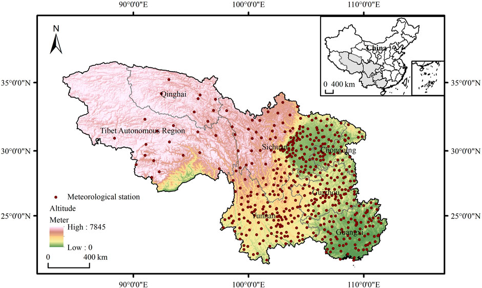
FIGURE 1. Study area and 494 meteorological stations in Southwest China.

Data Sources

Meteorological Data

NSAT datasets during 1969–2018 were downloaded from China Meteorological Data Service Center (http://data.cma.cn), covering 494 meteorological stations in Southwest China (Table 1). Its quality and uniformity were assessed by the National Meteorological Information Center. The data include daily and monthly averages, maximum and minimum temperatures. The annual and seasonal temperatures for each station were obtained by averaging the corresponding month temperatures. Specifically, the spring (T_spring), summer (T_summer), autumn (T_autumn), and winter (T_winter) denote the averages of March–May, June–August, September–November, and December–February, respectively.

TABLE 1

TABLE 1. Datasets used to analyze NSAT in Southwest China.

Terrain Morphology Data

The Digital Elevation Model (DEM) at the spatial resolution of 90 m that was measured by the NASA Shuttle Radar Topographic Mission (SRTM). The DEM data were collected from the Computer Network Information Center, Chinese Academy of Sciences (http://www.gscloud.cn). In this study, the measures used were elevation, slope, and aspect. Prior to formal interpolation, we evaluated the performances of the DEM data with different spatial resolutions. We noticed that with the resolution of 500 m, the interpolation process can be completed with speed and the quality was satisfactory. Thus, all the terrain data were resampled to 500 m × 500 m, and the medians in each grid cell were used.

Other Air Temperature Datasets

The monthly mean near surface air temperature data for 1970–2000 on a 30 arc-second resolution grid were obtained from the WorldClim Data Portal (https://www.worldclim.org). The gridded data sets cover China at 1 km × 1 km resolution (HMTC) for the same period (Peng et al., 2019) were obtained from the National Earth System Science Data Center (http://www.geodata.cn). Specifically, WorldClim dataset is a set of global climate layers, while HMTC dataset was spatially downscaled from the 30 arc-minute resolution Climatic Research Unit (CRU) time series dataset. These reference datasets could provide detailed climatology data, and could be evaluated against the land-based observations. Moreover, they could reflect orographic effects, and are available for monthly mean, minimum and maximum NSATs.

Methodology

Improved ANUSPLIN Model

The ANUSPLIN is created using thin-plate smoothing splines, which make it suitable for interpolating climate data with large noises (Hutchinson and Gessler, 1994; Price et al., 2000; Guo et al., 2020). The noisy multivariable climatic data are treated as a function with one or more independent variables during the fitting process of a climatic surface, and thus can produce mean error lower than other interpolation methods (Islam and Déry, 2017; Zhao et al., 2019; Cheng et al., 2020). The theoretical statistical model is expressed as:

${\text{Z}}_i=f\left(x_i\right)+b^T{y}_i+e_i\left(i=1,\dots ,N\right)(1)$

where Z_i represents the predicted value at location i; x_i is the spline independent variable as a multidimensional vector, and f represents a smoothing function of x_i which needs to be estimated; y_i is the independent covariable as a multidimensional vector, and b is the unknown coefficients for the y_i; n is the number of observational data. Each e_i is an independent, zero mean error term with variance w_iσ², where W_i is the known relative error variance and σ² is the error variance which is constant across all data points.

The traditional ANUSPLIN treats longitude and latitude as independent variables, with elevation as a covariate. To optimize the ANUSPLIN model, we improved it by incorporating more terrain-related factors, with slope, and aspect also as covariates (hereafter called M-ANUSPLIN).

Interpolation Methods

The NSAT parameters in Southwest China are estimated using co-kriging, ANUSPLIN and M-ANUSPLIN models, respectively. Due to the complex topography of the domain over Southwest China, we tested the performance of these models using different combinations of covariates (Table 4) to identify the best model in this region, and to find which variable contributes more to NSAT variability.

Model Assessment

To evaluate these models, a 10-fold cross validation test was conducted to assess the overall error of the interpolated NSAT grid. The advantage of 10-fold cross validation is that all observations are used for both training and validation, and each observation is used for validation exactly once. Thus, it is widely used to validate gridded observations (Appelhans et al., 2015; Yoo et al., 2018). In 10-fold cross validation for this study, the original observation data of 494 meteorological stations were randomly partitioned into ten subsamples. Of the ten subsamples, a single subsample was retained as the validation data for testing the model, and the remaining nine subsamples were used as training data. The cross validation process was then repeated ten times, with each of the ten subsamples used exactly once as the validation data. Hence, 10 different combinations of training and test sets were formed, and each of training and test pair was applied and evaluated. Final evaluation of 10-fold cross validation test was determined by the average mis-classification probability over the ten test sets to produce a single estimation.

Based on the results of 10-fold cross validation test, the statistical indices of Mean Absolute Error (MAE), Root Mean Square Error (RMSE) and R-squared (R²) between predicted and observed values were selected as interpolation performance evaluation criteria. Briefly, MAE provides a measure of how far the estimate can be in error; RMSE provides a measure that is, sensitive to outliers; and R² provides the proportion of variation that is, explained by the predictor variables. The performance and bias were then compared by using the three indices, and the interpolation method with better performance was further selected. The calculation formulas of them are shown below:

$MAE=\frac{1}{n}{\displaystyle \sum _{i=1}^n\left|P_i-O_i\right|}(2)$

$RMSE=\sqrt{\frac{1}{n}{{\displaystyle \sum _{i=1}^n\left(P_i-O_i\right)}}^2}(3)$

$R^2=1-\frac{{\displaystyle {\sum }_{i=1}^n{\left(P_i-O_i\right)}^2}}{{\displaystyle {\sum }_{i=1}^n{\left(O_i-\overline{O}\right)}^2}}(4)$

where P_i and O_i are the estimated NSAT and original observational NSAT at each station, respectively; $\overline{O}$ is the mean of observational NSAT; and n is the sample number.

Accuracy Comparison

To further examine the accuracy of obtained data set, two published and widely used air temperature products were compared. One is the 30 arc-second resolution grid product obtained from WorldClim Data Portal (hereafter called WorldClim2), the other is the gridded data sets cover China at 1 km × 1 km resolution (hereafter called HMTC). Mean temperature values in time series of 1970–2000 derived from all datasets were compared. The M-ANUSPLIN and WorldClim2 values were resampled to 1 km × 1 km to render them consistent with the HMTC reference products.

Trend Analysis

A trend slope ratio analysis was examined to investigate the changing trends of NSAT for each pixel in 1969–2018 at both annual and seasonal scales. The formula is as follows (Vogelsang and Nawaz, 2017):

$slope=\frac{n\times {\displaystyle {\sum }_{i=1}^{n}i\times Te{m}_i}-{\displaystyle {\sum }_{i=1}^{n}i}{\displaystyle {\sum }_{i=1}^{n}Te{m}_i}}{n\times {\displaystyle {\sum }_{i=1}^n{i}^2}-{\left({\displaystyle {\sum }_{i=1}^{n}i}\right)}^2}(5)$

where slope is the degree of change in Tem; n is the number of studied years; i is the order of year from 1 to 50 in the study period; and Tem_i is the average Tem in the ith year. Slope >0 means that the air temperature over n years increased (warming trend); while slope<0 signifies a decreasing trend (cooling trend). To test the significance of these trends, a significance test (F-test) was applied. According to the F-test, the trends were divided into categories of extremely significant (p < 0.01), significant (0.01 < p< 0.05), and non-significant level (p > 0.05).

A coefficient of variation (CV) index was also considered to evaluate the spatio-temporal variation of NSAT. The CV was calculated as follows (Yang and Jiang, 2017):

$CV=\frac{1}{\overline{Tem}}\times \sqrt{\frac{1}{n-1}{\displaystyle \sum _{i=1}^n{\left(Te{m}_i-\overline{Tem}\right)}^2}}\times 100\%(6)$

where CV is the coefficient of variation for NSAT; $\overline{Tem}$ is the mean temperature; Tem_i is the temperature for year i; n is the number of studied years; i is the order of year from 1 to 50 in the study period. The significance test is carried out based on the p value. The CV is classified into three categories of weak variation (0 < CV ≤ 10%), medium variation (10% < CV ≤ 100%) and strong variation (CV > 100%).

Change Points Detection

For a long-term climatic dataset, it is expected to experience multiple changes rather than a single break (Khapalova et al., 2018). To detect and identify the time when significant changes for NSAT happened in the time series of 1969–2018, pruned exact linear time (PELT) was also conducted in this study. The superiority of PELT exists in the ability of accurate and fast detection and identification of multiple change-points (Killick et al., 2012).

Results

Model Performance

Table 2 compares the MAE, RMSE and R² of the predicted NSAT parameters using different models over Southwest China in 1969–2018. Apparently, the prediction of M-ANUSPLIN model gave lower MAE and RMSE compared to the ANUSPLIN and co-kriging models for both annual and seasonal NSATs. The R² values of the M-ANUSPLIN model were 0.077–0.328°C above those of the other two models. Specifically, for annual parameters, relative to the ANUSPLIN and co-kriging models, the MAEs and RMSEs for the M-ANUSPLIN model were 0.02–0.04°C lower for mean temperature (T_mean); 0–0.02°C lower for maximum temperature (T_max); and 0.03–0.07°C lower for minimum temperature (T_min). For seasonal parameters, the MAEs and RMSEs for the M-ANUSPLIN model were also 0.01–0.04°C and 0–0.05°C lower than the ANUSPLIN and co-kriging models. These results indicate the improvement of the M-ANUSPLIN model by incorporating slope and aspect as interpolators. Moreover, Table 2 also reflects the seasonal dependence of the model performance. In general, the MAEs and RMSEs decline in the order from winter to autumn to spring then to summer, while the R² basically has the opposite trend.

TABLE 2

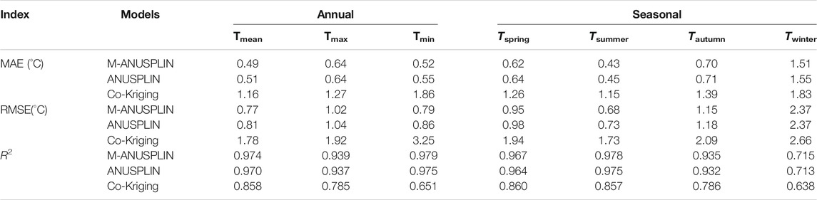
TABLE 2. 10-fold cross-validation results of the co-kriging, ANUSPLIN, and M-ANUSPLIN models.

Figure 2 and Table 3 show the performances of co-kriging, ANUSPLIN and M-ANUSPLIN models along altitudinal gradients. It can be seen that in general, the M-ANUSPLIN model has obvious advantages in regions with altitude <4,000 m, followed by the ANUSPLIN and co-kriging models. However, with the exception of elevation >4000 m, the MAE and RMSE of the M-ANUSPLIN model were slightly higher than those of the ANUSPLIN model. Moreover, in areas with altitude >4,000 m, all the three models generally gave overestimated values.

FIGURE 2

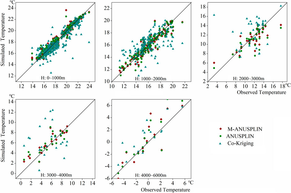
FIGURE 2. The MAEs of co-kriging, ANUSPLIN, and M-ANUSPLIN models along altitudinal gradients.

TABLE 3

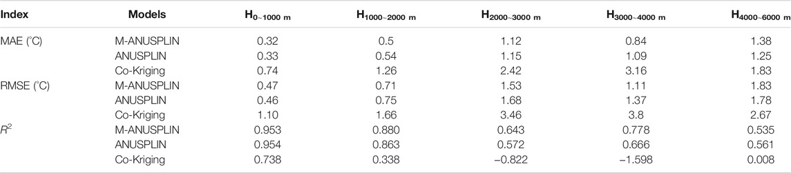
TABLE 3. Accuracy metrics of co-kriging, ANUSPLIN, and M-ANUSPLIN for the different altitudinal gradients.

A summary of the performances of the ANUSPLIN and M-ANUSPLIN models were further compared using different combinations of covariates (Table 4). It can be seen that the incorporation of additional terrain-related factors resulted in more accurate results, and slope angle contribute more to NSAT than slope orientation.

TABLE 4

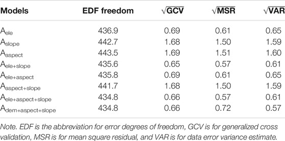
TABLE 4. Comparisons of the ANUSPLIN model using different combinations of covariates.

Temporal Variation

Trends of Annual Temperature

The magnitude of change for annual mean NSAT ranged 15.20–16.81°C. Figure 3 shows the annual variation of NSAT in the last 5 decades in Southwest China. It can be seen that over the whole region, with respect to the mean temperature during the period 1969–2018, the anomalies of mean temperature (T_mean) ranged −0.80 to 0.80°C; maximum temperature (T_max) ranged −0.93 to 1.07°C; while minimum temperature (T_min) ranged −0.77 to 0.96°C. In addition, T_mean, T_max, and T_min increased by 0.21°C/decade, 0.23°C/decade, and 0.28°C/decade over the past 50 years, respectively. Moreover, the warming rates for minimum temperature (0.28°C/decade) were greater than those for maximum temperature (0.23°C/decade), with T_min about 1.22 times of T_max.

FIGURE 3

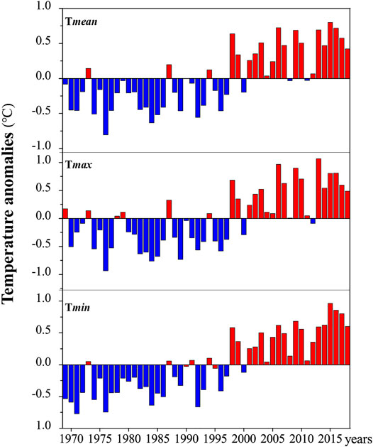
FIGURE 3. Annual variations of NSAT anomalies in Southwest China for the period 1969–2018.

Trends of Seasonal Temperature

The changes of seasonal NSAT for spring, summer, autumn and winter were 15.54–18.06°C, 22.15–24.13°C, 14.63–16.82°C, and 6.26–8.88°C, respectively. Figure 4 indicates the similarity between the temporal patterns of the seasonal NSAT and the annual NSAT trends. Nevertheless, compared with annual NSAT, the temporal variations of seasonal NSAT could not be divided into cooling and warming phases clearly. Specifically, the temperature variations in summer were more stable than that in other seasons. Moreover, for spring, autumn and winter, the temperature variations showed stronger inter-annual fluctuations. This could lead to extreme weather events in Southwest China.

FIGURE 4

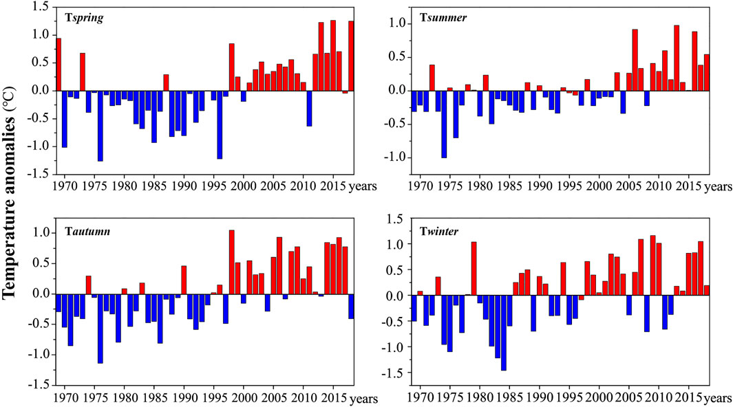
FIGURE 4. Seasonal variations of NSAT anomalies in Southwest China for the period 1969–2018.

In Figure 4, the warming rate in summer (0.16°C/decade) was lower than those in spring (0.22°C/decade), winter (0.22°C/decade), and autumn (0.23°C/decade). This means that the most unnotable contribution to the warming in Southwest China as a whole comes from summer.

Change-Points of NSAT

Annual and seasonal variations of NSAT anomalies show that the overall warming over Southwest China started in the late 1990s and accelerated after it (Figures 3, 4). Specifically, for mean temperature (T_mean), 18 out of 21 years were above the long-term average after 1998, while it was 3 out of 29 before 1998. This indicates that the NSAT of Southwest China was characterized by the transitions from cold to warm phases in the late 1990s.

To detect and identify the time when significant changes of NSAT occurred, the significant changes of each NSAT parameters were identified by using the PELT method at both annual and seasonal scales (as shown in Figure 5). It can be seen that the annual changes for maximum, average and minimum NSATs were quite similar to the seasonal changes. Moreover, there is strong evidence for the changes in all variables in the late 1990s and early 2000s. Specifically, for the annual mean temperature (T_mean) and maximum temperature (T_max), the significant changes began after 1997. While for the minimum temperature (T_min), there were two significant change points with both of them indicating a warming phase. The first change also started after 1997, and the second change began after 2011. Regarding the seasonal parameters, the change began after 1997, 2004, 1997, and 1985 for spring, summer, autumn and winter, respectively.

FIGURE 5

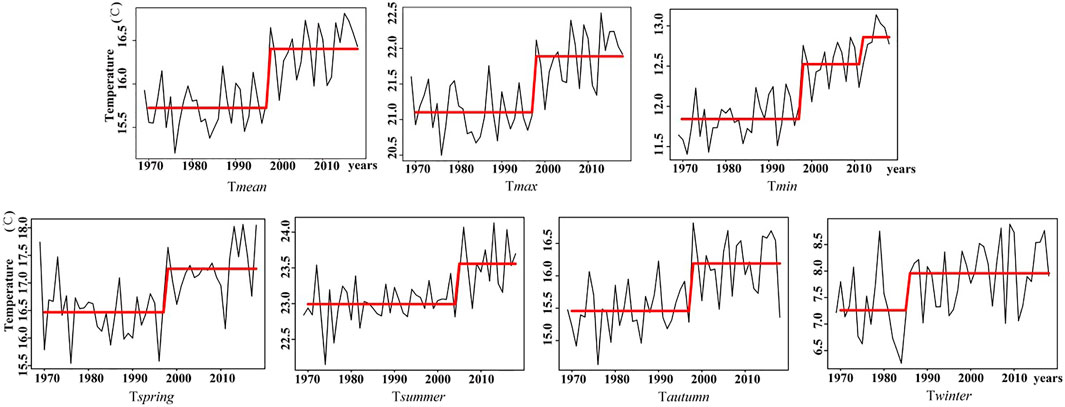
FIGURE 5. Change-points for annual and seasonal NSATs in Southwest China for the period 1969–2018 (p-value < 0.05).

Overall, it is clear that most of the significant changes of NSAT occurred either in the late 1990s or in the early 2000s. Thus, in terms of NSAT variations, the late 1990s and early 2000s can be remarked as the abrupt change period in Southwest China.

Spatial Variation of NSAT

To further probe into the spatial variation patterns of annual and seasonal NSATs over Southwest China, the variations with significance test were analyzed at the pixel scale. The area proportions occupied by extremely significant, significant and non-significant NSAT related indices are shown in Figures 6, 7. It can be seen that the M-ANUSPLIN interpolation datasets can capture the detailed NSAT very well, and they can accurately represent the climate characteristics in Southwest China, such as the extremely significant cooling regions with high elevations (e.g., the northwest of Qinghai-Tibet Plateau), the non-significant warming regions with low elevations (e.g., the northeast of Sichuan Basin), and extremely significant warming regions in most part of the study area. Moreover, despite slight differences between the spatial variations of annual NSAT and those of the seasonal indices, they exhibited highly consistent characteristics. Specifically, for the mean annual NSAT, during the period 1969–2018, 85.66% of the study area showed extremely significant warming with the most notable increases in the southeast region. Areas occupied by non-significant warming accounted for 2.48%, followed by significant warming with 1.32%, leading to an overall warming tendency across Southwest China. Nevertheless, the northwest region experienced a contrary characteristic, with extremely significant, and significant cooling accounted for 8.35%. This could be attributed to the high altitude in this region, which belongs to the Qinghai-Tibetan Plateau. Regarding the mean seasonal NSAT, areas occupied by extremely significant warming in spring, summer, autumn and winter accounted for 63.48, 71.47, 72.36 and 54.77%, respectively. Otherwise, it can be seen that winter has the highest proportions for non-significant warming, comparing to other seasons (Figure 7).

FIGURE 6

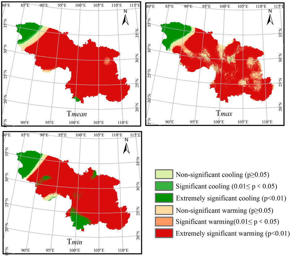
FIGURE 6. Trends of annual NSAT over Southwest China for the period 1969–2018. Panels (A–C) correspond to the mean annual, mean annual maximum, and minimum temperatures, respectively.

FIGURE 7

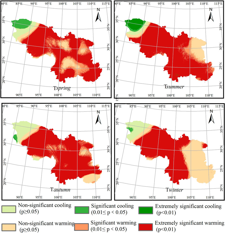
FIGURE 7. Trends of NSAT over southwest China for the period 1969–2018. Panels (A–D) correspond to the mean spring, summer, autumn, and winter NSATs, respectively.

Figure 8 shows the coefficient maps of variation (CV) index for NSAT over Southwest China. It indicates the high consistency of the CV index of annual NSAT with that of seasonal index over the past 50 years. Both annual and seasonal CV indices were generally stable and mainly dominated by weak or medium variations. Strong variations were mainly observed in high altitude regions, or in the combined section for encompassing plain and mountainous regions. For seasonal NSAT indices, it also mainly exhibited weak or medium variations, with different patterns in different seasons. Specifically, strong variations were identified in autumn and spring, followed by winter, while summer was the most stable, denoting that autumn maybe more susceptible to the warming.

FIGURE 8

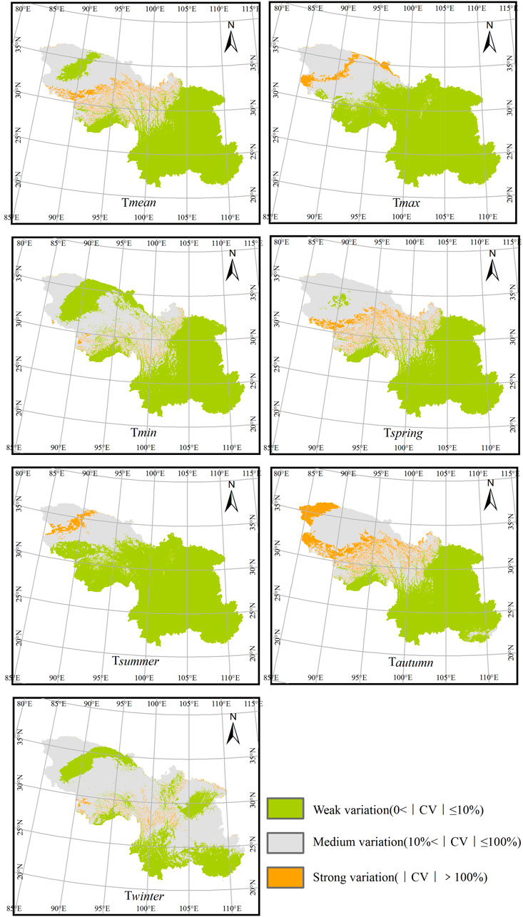
FIGURE 8. Coefficient of variation (CV) index for NSAT over Southwest China for the period 1969–2018. Panels (A–G) correspond to the mean annual, mean annual maximum, mean annual minimum, mean spring, mean summer, mean autumn, and mean winter NSATs, respectively.

Discussion

Priority of M-ANUSPLIN

Previous studies indicated that topographic information might be the key factor in climate indices prediction, especially in mountainous or high altitude areas with low density of meteorological stations (Gao et al., 2018; Peng et al., 2019). Therefore, it is possible that the precision of interpolation could be further improved by incorporating more detail terrain-related factors (Cheng et al., 2020). Nevertheless, traditional interpolation method is usually processed under the assumption that the NSAT is only dependent on the altitude. However, Šafanda (1999) demonstrated the strong dependence of NSAT on slope angle and orientation. Therefore, it is possible that the precision of interpolation for NSAT could be improved by considering slope angle and orientation in the interpolation process.

In this study, we included longitude and latitude as independent variables, and incorporated elevation, slope and aspect as covariates. We found that compared to the ANUSPLIN model, the MAE and RMSE values decreased by 0–5.77 and 1.96–8.86% for annual parameters, and 1.43–4.65 and 0–7.35% for seasonal parameters. As a result, the M-ANUSPLIN exhibited smaller deviation and performed better against other interpolation methods, especially in mountainous regions. However, our results also reflected the relatively poor performance of the M-ANUSPLIN model in regions with altitude >4,000 m, suggesting that it is not optimal for all regions.

Our study confirmed that slope is an important terrain-related factor in the interpolation process for NSAT (Table 4). As slope angle affects the temperature of surface objects by influencing the incidence angle and reflectivity of solar radiation, and then alters NSAT (Li et al., 2015; Peng et al., 2020). However, our study revealed the much smaller contribution of slope orientation to NSAT estimation than slope angle. This is not consistent with existing knowledge, which believes that slope orientation plays an important role in NSAT prediction. Earlier studies reported that in the middle latitudes of the Northern Hemisphere, the north slopes are generally colder at the same elevation than the south slopes because sunny aspects receive more direct solar radiation than northern aspects (Šafanda, 1999; Li et al., 2015). One reason for this inconsistent might be due to the different vegetation types in Southwest China. For example, Šafanda (1999) explained that the surface temperature in the meadow is higher than that in the forest because much of the Sun radiation is absorbed by the trees. Thus, the NSAT for meadows located at north slopes might be higher than the NSAT for forests located at south slopes. Another reason might be due to the existence and duration of the snow cover in high altitude regions, which can offset the effects of slope orientation on NSAT. Consequently, the effect of slope orientation on NSAT in Southwest China was smaller compared to those in other regions.

Comparisons With Other Datasets

To examine the accuracy of M-ANUSPLIN interpolated dataset, the predicted results were compared to both the WorldClim 2.0 dataset (Fick and Hijmans, 2017) and the HMTC dataset (Peng et al., 2019). The 10-fold cross validation test was used to evaluate the overall error of the interpolated NSAT grid obtained from each dataset and the original observation data of 494 meteorological stations (Table 5).

TABLE 5

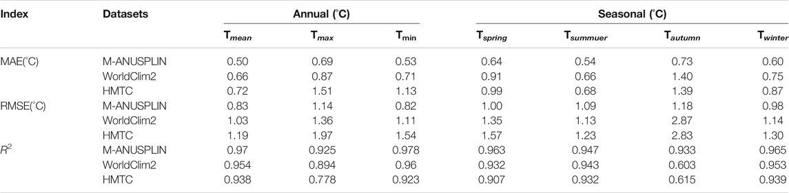
TABLE 5. Comparisons of annual and seasonal climatology indices among different datasets.

Table 5 lists the mean, maximum, minimum values for annual and seasonal NSAT variables obtained from different datasets. It can be seen that the climatology anomaly of M-ANUSPLIN dataset is the lowest comparing to the WorldClim 2.0 and the HMTC datasets. Specifically, the anomalies are relatively high for HMTC (0.72–1.51°C for MAE and 1.19–1.97°C for RMSE); intermediate for WorldClim2 (0.66–0.87°C for MAE and 1.03–1.36°C for RMSE); and the lowest for M-ANUSPLIN (0.50–0.69°C for MAE and 0.82–1.14°C for RMSE). The seasonal NSAT variables shows the similar trend, where HMTC gives the highest estimation error, followed by WorldClim2 and M-ANUSPLIN. The good performance of M-ANUSPLIN can be mainly attributed to two reasons. Firstly, in case of WorldClim2 and HMTC datasets, only ∼300 sites and ∼500 sites of in-situ observation stations were respectively used for interpolation, and therefore significant biases occurred due to the complex terrain (Peng et al., 2019). Secondly, the M-ANUSPLIN model incorporated more detailed topographic information than traditional models, and thus can capture NSAT features with better precision.

Overall, the results indicate that the improved M-ANUSPLIN model can produce more accurate NSAT values than traditional interpolation models, and has apparent advantages over other interpolation methods in complex terrain areas like Southwest China.

Study Limitations

Whilst this study demonstrated that the improved M-ANUSPLIN method can estimate more accurate NSAT than traditional models, especially in complex terrain areas like Southwest China, uncertainties still remain regarding the density of meteorological stations, input datasets and urbanization effect. Firstly, as gauge stations are relatively sparse in the western region of the study area, acquiring a correct distribution of NSAT through interpolation is difficult. The interpolated NSAT grid surface might contain some biases, which could introduce some uncertainty, especially in regions where the NSAT varies significantly in space and time. In addition, as the satellite SRTM product represents the average value in a 500 m × 500 m pixel, it does not provide the fine details and thus could not fully represent the real situation, which might also lead to additional biases.

Secondly, another source of uncertainty could be due to the input datasets. The NSAT is affected not only by topographical factors, but also closely related to other factors, e.g., vegetation and soil (Cho and Choi, 2014; Lensky et al., 2018). Moreover, as mentioned above, the effects of snow cover could be stronger than general expectation. It implies the need of careful interpretation of NSAT. Therefore, to further improve the accuracy of NSAT prediction, more information should be taken into account in the future.

Thirdly, the urbanization heat effect, which has a strong warming effect on NSAT (Kalnay and Cai, 2003; Ren et al., 2008; Luo and Lau, 2021), has not been considered in this study. This could cause an underestimation of NSAT, especially in the eastern region of Southwest China with a lot of big cities. Nonetheless, the results of this work should still, at least qualitatively, reveal the trends and spatial-temporal variations of NSAT in Southwest China over the past 50 years.

Lastly, elevation is an important factor affecting spatial variability of climate (Pepin et al., 2015). It is well known that for a stationary atmosphere, an increase in elevation leads to a subsequent decrease in air pressure and NSAT (You et al., 2008). According to EI Kenawy et al., 2009, different regions can experience different variations of NSAT, as each region has a unique terrain (Limsakul & Goes, 2008). Moreover, the variation of NSAT was not consistent between high and low land areas. Many studies suggested that NSAT increased more rapidly at higher than at lower elevations (Beniston, 2003; You et al., 2008; Pepin et al., 2015), which has been defined as elevation-dependent warming (EDW). However, this faster warming is not ubiquitous across the globe (Thakuri et al., 2019). In general, this study agrees with the previous studies of the EDW phenomenon with most high-altitude areas show significant warming. Nevertheless, we also observed a significant cooling trend in some high altitude regions like the northwestern part of Southwest China in the past 50 years. The reason for this phenomenon is still unclear, thus further investigation would be required.

Conclusion

This study enhanced the ANUSPLIN model by incorporating elevation, slope angle and orientation as covariates; and constructed monthly NSAT datasets with a spatial resolution of 500 m in Southwest China from January 1969 to December 2018. The accuracy of the M-ANUSPLIN model was evaluated by analyzing error statistics based on comparisons between interpolated values against withheld stations data. Furthermore, we compared the M-ANUSPLIN predicted dataset against existing datasets. To our knowledge, this is one of the few studies which considered slope angle and orientation to account for the terrain effects on NSAT. The independent validation results confirmed the clear advantages of the optimized M-ANUSPLIN model against other interpolation methods in Southwest China. Our methodology therefore represents a significant and practical improvement in NSAT estimation. Therefore, it has great potential for meteorological and climatological research, especially in mountainous regions with diverse topography.

As mentioned above, during the period 1969–2018, consistent warming and significant EDW were found in most part of Southwest China, while some sporadic areas like northwestern region exhibited opposite trends. In general, Southwest China experienced an overall warming with a rate of 0.21°C/decade, obviously higher than mainland China and global averages. This implies that Southwest China is more sensitive to global warming than generally recognized. The warming mainly started in the late 1990s, and the hiatus or slowdown phenomenon was not observed as expected, and the NSAT experienced a persistent and even more significant warming after the 1997/1998 EL Niño event. This means that climate change in Southwest China should be of particular concern. Moreover, the increase of low temperature was significantly greater than that of high temperature, where the warming rate of T_min (0.28°C/decade) about 1.22 times of T_max (0.23°C/decade); and that of T_winter (0.22°C/decade) about 1.38 times of T_summer (0.16°C/decade). These indicate that the increases of T_min and T_winter contribute the most to the warming effect in Southwest China over the past 50 years.

Data Availability Statement

The raw data supporting the conclusion of this article will be made available by the authors, without undue reservation.

Author Contributions

JZ and TL conceived the study, performed the analysis, drafted the manuscript; TL supervised the project. All authors listed have made a substantial, direct, and intellectual contribution to the work and approved it for publication.

Funding

This research was supported by the Second Tibetan Plateau Scientific Expedition and Research program (2019QZKK04020301), the National Natural Science Foundation of China (42071238, 41371126), the Program for Biodiversity Protection of Ministry of Ecology and Environment of the People’s Republic of China (9311341), the National Key Research and Development Program of China (2016YFC0502101).

Conflict of Interest

The authors declare that the research was conducted in the absence of any commercial or financial relationships that could be construed as a potential conflict of interest.

Publisher’s Note

All claims expressed in this article are solely those of the authors and do not necessarily represent those of their affiliated organizations, or those of the publisher, the editors and the reviewers. Any product that may be evaluated in this article, or claim that may be made by its manufacturer, is not guaranteed or endorsed by the publisher.

References

Amato, R., Steptoe, H., Buonomo, E., and Jones, R. (2019). High-Resolution History: Downscaling China's Climate from the 20CRv2c Reanalysis. J. Appl. Meteorol. Clim. 58 (10), 2141–2157. doi:10.1175/JAMC-D-19-0083.1

CrossRef Full Text | Google Scholar

Appelhans, T., Mwangomo, E., Hardy, D. R., Hemp, A., and Nauss, T. (2015). Evaluating Machine Learning Approaches for the Interpolation of Monthly Air Temperature at Mt. Kilimanjaro, Tanzania. Spat. Stat. 14, 91–113. doi:10.1016/j.spasta.2015.05.008

CrossRef Full Text | Google Scholar

Belkhiri, L., Tiri, A., and Mouni, L. (2020). Spatial Distribution of the Groundwater Quality Using Kriging and Co-kriging Interpolations. Groundwater Sustain. Dev. 11, 100473. doi:10.1016/j.gsd.2020.100473

CrossRef Full Text | Google Scholar

Beniston, M. (2003). Climatic Change in Mountain Regions: A Review of Possible Impacts. Climatic Change 59, 5–31. doi:10.1007/978-94-015-1252-7_2

CrossRef Full Text | Google Scholar

Cahill, N., Rahmstorf, S., and Parnell, A. C. (2015). Change Points of Global Temperature. Environ. Res. Lett. 10 (8), 084002. doi:10.1088/1748-9326/10/8/084002

CrossRef Full Text | Google Scholar

Chen, X., Li, N., Zhang, Z., Feng, J., and Wang, Y. (2018). Change Features and Regional Distribution of Temperature Trend and Variability Joint Mode in mainland China. Theor. Appl. Climatol 132 (3-4), 1049–1055. doi:10.1007/s00704-017-2148-z

CrossRef Full Text | Google Scholar

Cheng, J., Li, Q., Chao, L., Maity, S., Huang, B., and Jones, P. (2020). Development of High Resolution and Homogenized Gridded Land Surface Air Temperature Data: A Case Study over Pan-East Asia. Front. Environ. Sci. 8, 588570. doi:10.3389/fenvs.2020.588570

CrossRef Full Text | Google Scholar

Cho, E., and Choi, M. (2014). Regional Scale Spatio-Temporal Variability of Soil Moisture and its Relationship with Meteorological Factors over the Korean peninsula. J. Hydrol. 516, 317–329. doi:10.1016/j.jhydrol.2013.12.053

CrossRef Full Text | Google Scholar

Collados-Lara, A.-J., Fassnacht, S. R., Pardo-Igúzquiza, E., and Pulido-Velazquez, D. (2021). Assessment of High Resolution Air Temperature Fields at Rocky Mountain National Park by Combining Scarce Point Measurements with Elevation and Remote Sensing Data. Remote Sensing 13 (1), 113. doi:10.3390/rs13010113

CrossRef Full Text | Google Scholar

Cuervo-Robayo, A. P., Téllez-Valdés, O., Gómez-Albores, M. A., Venegas-Barrera, C. S., Manjarrez, J., and Martínez-Meyer, E. (2014). An Update of High-Resolution Monthly Climate Surfaces for Mexico. Int. J. Climatol. 34 (7), 2427–2437. doi:10.1002/joc.3848

CrossRef Full Text | Google Scholar

Cui, L. L., Shi, J., Du, H. Q., and Wen, K. M. (2017). Characteristics and Trends of Climatic Extremes in China during 1959-2014. J. Trop. Meteorol. 23 (4), 368–379. 1006-8775(2017) 04-0368-12.

Google Scholar

Cui, L., and Shi, J. (2021). Evaluation and Comparison of Growing Season Metrics in Arid and Semi-arid Areas of Northern China under Climate Change. Ecol. Indicators 121, 107055. doi:10.1016/j.ecolind.2020.107055

CrossRef Full Text | Google Scholar

Diaz, H. F., and Bradley, R. S. (1997). Temperature Variations during the Last century at High Elevations Sites. Climatic Change 36 (3-4), 253–279. doi:10.1023/A:1005335731187

CrossRef Full Text | Google Scholar

Ding, Y., Ren, G., ZhaoXu, Z. Y., Xu, Y., Luo, Y., Li, Q., et al. (2007). Detection, Causes and Projection of Climate Change over China: An Overview of Recent Progress. Adv. Atmos. Sci. 24 (6), 954–971. doi:10.1007/s00376-007-0954-4

CrossRef Full Text | Google Scholar

Dong, D., Huang, G., Qu, X., Tao, W., and Fan, G. (2015). Temperature Trend-Altitude Relationship in China during 1963-2012. Theor. Appl. Climatol. 122, 285–294. doi:10.1007/s00704-014-1286-9

CrossRef Full Text | Google Scholar

Du, H., Hu, F., Zeng, F., Wang, K., Peng, W., Zhang, H., et al. (2017). Spatial Distribution of Tree Species in evergreen-deciduous Broadleaf Karst Forests in Southwest China. Sci. Rep. 7, 15664. doi:10.1038/s41598-017-15789-5

PubMed Abstract | CrossRef Full Text | Google Scholar

Du, Q., Zhang, M., Wang, S., Che, C., Ma, R., and Ma, Z. (2019). Changes in Air Temperature over China in Response to the Recent Global Warming Hiatus. J. Geogr. Sci. 29 (4), 496–516. doi:10.1007/s11442-019-1612-3

CrossRef Full Text | Google Scholar

Easterling, D. R., and Wehner, M. F. (2009). Is the Climate Warming or Cooling. Geophys. Res. Lett. 36, L08706. doi:10.1029/2009GL037810

CrossRef Full Text | Google Scholar

El Kenawy, A. M., López-Moreno, J. I., Vicente-Serrano, S. M., and Mekld, M. S. (2009). Temperature Trends in Libya over the Second Half of the 20th century. Theor. Appl. Climatol 98, 1–8. doi:10.1007/s00704-008-0089-2

CrossRef Full Text | Google Scholar

Fan, Z.-X., Bräuning, A., Thomas, A., Li, J.-B., and Cao, K.-F. (2011). Spatial and Temporal Temperature Trends on the Yunnan Plateau (Southwest China) during 1961-2004. Int. J. Climatol. 31 (14), 2078–2090. doi:10.1002/joc.2214

CrossRef Full Text | Google Scholar

Fick, S. E., and Hijmans, R. J. (2017). WorldClim 2: New 1‐km Spatial Resolution Climate Surfaces for Global Land Areas. Int. J. Climatol 37 (12), 4302–4315. doi:10.1002/joc.5086

CrossRef Full Text | Google Scholar

Fyfe, J. C., Meehl, G. A., England, M. H., Mann, M. E., Santer, B. D., Flato, G. M., et al. (2016). Making Sense of the Early-2000s Warming Slowdown. Nat. Clim Change 6 (3), 224–228. doi:10.1038/nclimate2938

CrossRef Full Text | Google Scholar

Gao, J., Jiao, K., and Wu, S. (2018). Quantitative Assessment of Ecosystem Vulnerability to Climate Change: Methodology and Application in China. Environ. Res. Lett. 13 (9), 094016. doi:10.1088/1748-9326/aadd2e

CrossRef Full Text | Google Scholar

Guo, B., Zhang, J., Meng, X., Xu, T., and Song, Y. (2020). Long-term Spatio-Temporal Precipitation Variations in China with Precipitation Surface Interpolated by ANUSPLIN. Sci. Rep. 10 (1), 81. doi:10.1038/s41598-019-57078-3

PubMed Abstract | CrossRef Full Text | Google Scholar

Hadi, S. J., and Tombul, M. (2018). Comparison of Spatial Interpolation Methods of Precipitation and Temperature Using Multiple Integration Periods. J. Indian Soc. Remote Sens 46 (7), 1187–1199. doi:10.1007/s12524-018-0783-1

CrossRef Full Text | Google Scholar

Hu, Z.-Z., Yang, S., and Wu, R. G. (2003). Long-term Climate Variations in China and Global Warming Signals. J. Geophys. Res. 108 (19), 4614. doi:10.1029/2003JD003651

CrossRef Full Text | Google Scholar

Hutchinson, M. F., and Gessler, P. E. (1994). Splines-more Than Just a Smooth Interpolator. Geoderma 62 (1-3), 45–67. doi:10.1016/0016-7061(94)90027-2

CrossRef Full Text | Google Scholar

Ilori, O. W., and Ajayi, V. O. (2020). Change Detection and Trend Analysis of Future Temperature and Rainfall over West Africa. Earth. Syst. Environ. 4 (3), 493–512. doi:10.1007/s41748-020-00174-6

CrossRef Full Text | Google Scholar

Islam, S. U., and Déry, S. J. (2017). Evaluating Uncertainties in Modelling the Snow Hydrology of the Fraser River Basin, British Columbia, Canada. Hydrol. Earth Syst. Sci. 21 (3), 1827–1847. doi:10.5194/hess-21-1827-2017

CrossRef Full Text | Google Scholar

Jiang, S., Liang, C., Cui, N., Zhao, L., Du, T., Hu, X., et al. (2019). Impacts of Climatic Variables on Reference Evapotranspiration during Growing Season in Southwest China. Agric. Water Manag. 216, 365–378. doi:10.1016/j.agwat.2019.02.014

CrossRef Full Text | Google Scholar

Jin, J., and Wang, Q. (2016). Assessing Ecological Vulnerability in Western China Based on Time-Integrated NDVI Data. J. Arid Land 8 (4), 533–545. doi:10.1007/s40333-016-0048-1

CrossRef Full Text | Google Scholar

Joly, D., Brossard, T., Cardot, H., Cavailhes, J., Hilal, M., and Wavresky, P. (2011). Temperature Interpolation Based on Local Information: the Example of France. Int. J. Climatol. 31 (14), 2141–2153. doi:10.1002/joc.2220

CrossRef Full Text | Google Scholar

Kalnay, E., and Cai, M. (2003). Impact of Urbanization and Land-Use Change on Climate. Nature 423 (6939), 528–531. doi:10.1038/nature01675

PubMed Abstract | CrossRef Full Text | Google Scholar

Khapalova, E. A., Jandhyala, V. K., Fotopoulos, S. B., and Overland, J. E. (2018). Assessing Change-Points in Surface Air Temperature over Alaska. Front. Environ. Sci. 6, 121. doi:10.3389/fenvs.2018.00121

CrossRef Full Text | Google Scholar

Khosravi, Y., and Balyani, S. (2019). Spatial Modeling of Mean Annual Temperature in Iran: Comparing Cokriging and Geographically Weighted Regression. Environ. Model. Assess. 24 (3), 341–354. doi:10.1007/s10666-018-9623-5

CrossRef Full Text | Google Scholar

Killick, R., Fearnhead, P., and Eckley, I. A. (2012). Optimal Detection of Changepoints with a Linear Computational Cost. J. Am. Stat. Assoc. 107, 1590–1598. doi:10.1080/01621459.2012.737745

CrossRef Full Text | Google Scholar

Lensky, I. M., Dayan, U., and Helman, D. (2018). Synoptic Circulation Impact on the Near-Surface Temperature Difference Outweighs that of the Seasonal Signal in the Eastern Mediterranean. J. Geophys. Res. Atmos. 123, 11333–11347. doi:10.1029/2017JD027973

CrossRef Full Text | Google Scholar

Lewandowsky, S., Cowtan, K., Risbey, J. S., Mann, M. E., Steinman, B. A., Oreskes, N., et al. (2018). Erratum: The 'pause' in Global Warming in Historical Context: II. Comparing Models to Observations (2018 Environ. Res. Lett . 13 123007). Environ. Res. Lett. 14 (4), 049601. doi:10.1088/1748-9326/aafbb7

CrossRef Full Text | Google Scholar

Li, J., and Heap, A. D. (2011). A Review of Comparative Studies of Spatial Interpolation Methods in Environmental Sciences: Performance and Impact Factors. Ecol. Inform. 6, 228–241. doi:10.1016/j.ecoinf.2010.12.003

CrossRef Full Text | Google Scholar

Li, Q., Sun, W., Yun, X., Huang, B., Dong, W., Wang, X. L., et al. (2021). An Updated Evaluation of the Global Mean Land Surface Air Temperature and Surface Temperature Trends Based on CLSAT and CMST. Clim. Dyn. 56 (1-2), 635–650. doi:10.1007/s00382-020-05502-0

CrossRef Full Text | Google Scholar

Li, X., Li, L., Yuan, S., Yan, H., and Wang, G. (2015). Temporal and Spatial Variation of 10-day Mean Air Temperature in Northwestern China. Theor. Appl. Climatol. 119 (1-2), 285–298. doi:10.1007/s00704-014-1100-8

CrossRef Full Text | Google Scholar

Li, Y., Zhang, D., Andreeva, M., Li, Y., Fan, L., and Tang, M. (2020). Temporal-spatial Variability of Modern Climate in the Altai Mountains during 1970-2015. Plos. One 15 (3), e0230196. doi:10.1371/journal.pone.0230196

PubMed Abstract | CrossRef Full Text | Google Scholar

Limsakul, A., and Goes, J. I. (2008). Empirical Evidence for Interannual and Longer Period Variability in Thailand Surface Air Temperatures. Atmos. Res. 87, 89–102. doi:10.1016/j.atmosres.2007.07.007

CrossRef Full Text | Google Scholar

Lin, P., He, Z., Du, J., Chen, L., Zhu, X., and Li, J. (2017). Recent Changes in Daily Climate Extremes in an Arid Mountain Region, a Case Study in Northwestern China's Qilian Mountains. Sci. Rep. 7, 2245. doi:10.1038/s41598-017-02345-4

PubMed Abstract | CrossRef Full Text | Google Scholar

Luo, M., and Lau, N.-C. (2017). Heat Waves in Southern China: Synoptic Behavior, Long-Term Change, and Urbanization Effects. J. Clim. 30 (2), 703–720. doi:10.1175/JCLI-D-16-0269.1

CrossRef Full Text | Google Scholar

Luo, M., and Lau, N. C. (2021). Increasing Human‐Perceived Heat Stress Risks Exacerbated by Urbanization in China: A Comparative Study Based on Multiple Metrics. Earth's Future 9, e2020EF001848. doi:10.1029/2020EF001848

CrossRef Full Text | Google Scholar

Minder, J. R., Mote, P. W., and Lundquist, J. D. (2010). Surface Temperature Lapse Rates over Complex Terrain: Lessons from the Cascade Mountains. J. Geophys. Res. 115, D14122. doi:10.1029/2009JD013493

CrossRef Full Text | Google Scholar

Mohammadi, S. A., Azadi, M., and Rahmani, M. (2017). Comparison of Spatial Interpolation Methods for Gridded Bias Removal in Surface Temperature Forecasts. J. Meteorol. Res. 31, 791–799. doi:10.1007/s13351-017-6135-1

CrossRef Full Text | Google Scholar

Nalder, I. A., and Wein, R. W. (1998). Spatial Interpolation of Climatic Normals: Test of a New Method in the Canadian Boreal forest. Agric. For. Meteorology 92 (4), 211–225. doi:10.1016/S0168-1923(98)00102-6

CrossRef Full Text | Google Scholar

Peng, S., Ding, Y., Liu, W., and Li, Z. (2019). 1 Km Monthly Temperature and Precipitation Dataset for China from 1901 to 2017. Earth Syst. Sci. Data 11 (4), 1931–1946. doi:10.5194/essd-11-1931-2019

CrossRef Full Text | Google Scholar

Peng, X., Wu, W., Zheng, Y., Sun, J., Hu, T., and Wang, P. (2020). Correlation Analysis of Land Surface Temperature and Topographic Elements in Hangzhou, China. Sci. Rep. 10 (1), 10451. doi:10.1038/s41598-020-67423-6

PubMed Abstract | CrossRef Full Text | Google Scholar

Pepin, N., Bradley, R. S., Diaz, H. F., Baraer, M., Caceres, E. B., Forsythe, N., et al. (2015). Elevation-dependent Warming in Mountain Regions of the World. Nat. Clim. Change 5, 424–430. doi:10.1038/nclimate2563

CrossRef Full Text | Google Scholar

Persaud, B. D., Whitfield, P. H., Quinton, W. L., and Stone, L. E. (2020). Evaluating the Suitability of Three Gridded‐datasets and Their Impacts on Hydrological Simulation at Scotty Creek in the Southern Northwest Territories, Canada. Hydrological Process. 34 (4), 898–913. doi:10.1002/hyp.13663

CrossRef Full Text | Google Scholar

Price, D. T., McKenney, D. W., Nalder, I. A., Hutchinson, M. F., and Kesteven, J. L. (2000). A Comparison of Two Statistical Methods for Spatial Interpolation of Canadian Monthly Mean Climate Data. Agr. For. Meteorol. 101 (2-3), 81–94. doi:10.1016/S0168-1923(99)00169-0

CrossRef Full Text | Google Scholar

Qian, H., Deng, T., Jin, Y., Mao, L., Zhao, D., and Ricklefs, R. E. (2019). Phylogenetic Dispersion and Diversity in Regional Assemblages of Seed Plants in China. Proc. Natl. Acad. Sci. USA 116 (46), 23192–23201. doi:10.1073/pnas.1822153116

PubMed Abstract | CrossRef Full Text | Google Scholar

Ren, G., Zhou, Y., ChuZhou, Z. J. X., Zhou, J., Zhang, A., Guo, J., et al. (2008). Urbanization Effects on Observed Surface Air Temperature Trends in north China. J. Clim. 21 (6), 1333–1348. doi:10.1175/2007JCLI1348.1

CrossRef Full Text | Google Scholar

Ren, Y., Parker, D., Ren, G., and Dunn, R. (2016). Tempo-spatial Characteristics of Sub-daily Temperature Trends in mainland China. Clim. Dyn. 46 (9-10), 2737–2748. doi:10.1007/s00382-015-2726-7

CrossRef Full Text | Google Scholar

Risbey, J. S., Lewandowsky, S., Cowtan, K., Oreskes, N., Rahmstorf, S., Jokimäki, A., et al. (2018). A Fluctuation in Surface Temperature in Historical Context: Reassessment and Retrospective on the Evidence. Environ. Res. Lett. 13 (12), 123008. doi:10.1088/1748-9326/aaf342

CrossRef Full Text | Google Scholar

Šafanda, J. (1999). Ground Surface Temperature as a Function of Slope Angle and Slope Orientation and its Effect on the Subsurface Temperature Field. Tectonophysics 306, 367–375. doi:10.1016/S0040-1951(99)00066-9

CrossRef Full Text | Google Scholar

Sun, X., Ren, G., Ren, Y., Fang, Y., Liu, Y., Xue, X., et al. (2018). A Remarkable Climate Warming Hiatus over Northeast China since 1998. Theor. Appl. Climatol. 133 (1-2), 579–594. doi:10.1007/s00704-017-2205-7

CrossRef Full Text | Google Scholar

Tang, G. L., Luo, Y., Huang, J. B., Wen, X. Y., Zhu, Y. N., Zhao, Z. C., et al. (2012). Continuation of the Global Warming. Clim. Chang. Res. 8 (4), 235–242. (in Chinese). doi:10.3969/j.issn.1673-1719.2012.04.001

CrossRef Full Text | Google Scholar

Tanır Kayıkçı, E., and Zengin Kazancı, S. (2016). Comparison of Regression-Based and Combined Versions of Inverse Distance Weighted Methods for Spatial Interpolation of Daily Mean Temperature Data. Arab. J. Geosci. 9 (17), 690. doi:10.1007/s12517-016-2723-0

CrossRef Full Text | Google Scholar

Thakuri, S., Dahal, S., Shrestha, D., Guyennon, N., Romano, E., Colombo, N., et al. (2019). Elevation-dependent Warming of Maximum Air Temperature in Nepal during 1976-2015. Atmos. Res. 228, 261–269. doi:10.1016/j.atmosres.2019.06.006

CrossRef Full Text | Google Scholar

Vogelsang, T. J., and Nawaz, N. (2017). Estimation and Inference of Linear Trend Slope Ratios with an Application to Global Temperature Data. J. Time Ser. Anal. 38 (5), 640–667. doi:10.1111/jtsa.12209

CrossRef Full Text | Google Scholar

Wang, M., He, G., Zhang, Z., Wang, G., Zhang, Z., Cao, X., et al. (2017). Comparison of Spatial Interpolation and Regression Analysis Models for an Estimation of Monthly Near Surface Air Temperature in China. Remote Sensing 9 (12), 1278. doi:10.3390/rs9121278

CrossRef Full Text | Google Scholar

Wang, S.-J. (2018). Spatiotemporal Variability of Temperature Trends on the Southeast Tibetan Plateau, China. Int. J. Climatol 38, 1953–1963. doi:10.1002/joc.5308

CrossRef Full Text | Google Scholar

Wu, T., and Li, Y. (2013). Spatial Interpolation of Temperature in the United States Using Residual Kriging. Appl. Geogr. 44, 112–120. doi:10.1016/j.apgeog.2013.07.012

CrossRef Full Text | Google Scholar

Xu, K., Wang, X., Jiang, C., and Sun, O. J. (2020). Assessing the Vulnerability of Ecosystems to Climate Change Based on Climate Exposure, Vegetation Stability and Productivity. For. Ecosyst. 7 (3), 23. doi:10.1186/s40663-020-00239-y

CrossRef Full Text | Google Scholar

Yang, K., and Jiang, D. (2017). Interannual Climate Variability Change during the Medieval Climate Anomaly and Little Ice Age in PMIP3 Last Millennium Simulations. Adv. Atmos. Sci. 34 (4), 497–508. doi:10.1007/s00376-016-6075-1

CrossRef Full Text | Google Scholar

Yoo, C., Im, J., Park, S., and Quackenbush, L. J. (2018). Estimation of Daily Maximum and Minimum Air Temperatures in Urban Landscapes Using MODIS Time Series Satellite Data. ISPRS J. Photogrammetry Remote Sensing 137, 149–162. doi:10.1016/j.isprsjprs.2018.01.018

CrossRef Full Text | Google Scholar

You, Q., Kang, S., Pepin, N., and Yan, Y. (2008). Relationship between Trends in Temperature Extremes and Elevation in the Eastern and central Tibetan Plateau, 1961-2005. Geophys. Res. Lett. 35, L14704. doi:10.1029/2007GL032669

CrossRef Full Text | Google Scholar

Zhao, H., Huang, W., Xie, T., Wu, X., Xie, Y., Feng, S., et al. (2019). Optimization and Evaluation of a Monthly Air Temperature and Precipitation Gridded Dataset with a 0.025° Spatial Resolution in China during 1951-2011. Theor. Appl. Climatol. 138 (1-2), 491–507. doi:10.1007/s00704-019-02830-y

CrossRef Full Text | Google Scholar

Zhou, Z., Shi, H., FuLi, Q. T. X., Li, T., Gan, T. Y., Liu, S., et al. (2020). Is the Cold Region in Northeast China Still Getting Warmer under Climate Change Impact. Atmos. Res. 237, 104864. doi:10.1016/j.atmosres.2020.104864

CrossRef Full Text | Google Scholar