3D Convolution Conjugate Gradient Inversion of Potential Fields in Acoculco Geothermal Prospect, Mexico

1 Introduction

Potential field data such as gravity and magnetics are among the first geophysical data used in mineral and hydrocarbon exploration. Their continued use has resulted in a historical improvement on data acquisition and interpretation methodologies as well as in the development of surveying instruments. One example is the development of modern airborne gravity gradiometers (Zhdanov et al., 2004; Nabighian et al., 2005; Dransfield and Zeng, 2009; Jekeli, 2006) and the increased use of unmanned aerial vehicles for aeromagnetic surveys (e.g., Aleshin et al., 2020; Jiang et al., 2020; Parshin et al., 2020; Walter et al., 2020). These technological developments have yielded the assimilation of the larger potential field data sets needed to achieve higher subsurface detail for reservoir, mineral, and archaeological studies.

Most algorithms for the numerical computation of the potential fields due to the arbitrarily shaped volumes are based on analytical responses of defined volumes such as rectangular prisms (Sorokin, 1951). Some examples of these algorithms are the 2D inversion linear programming developments by Mottl and Mottlová (1972), Cuer and Bayer (1980), and Safon et al. (1997). A complete review of existing algorithms for the computation of gravity and gravity gradient effects due to some geometric bodies such as rectangular prisms and polyhedrae can be found in Li and Chouteau (1998).

In order to carry out a large-scale data inversion, we need a fine three-dimensional discretization of the subsoil with a large number of parameters; thus, we need an efficient algorithm. Whereas exact analytical expressions allow the computation of arbitrarily shaped models, the reiterated computation of trigonometric and logarithm functions bears some computational cost. To face this challenge, several approaches have been developed. They include the extensive use of computational resources using parallel computing (e.g., Moorkamp et al., 2010) as well as various data-model compression strategies such as fast Fourier transform (e.g., Pilkington, 1997; Shin et al., 2006; Caratori Tontini et al., 2009), wavelet transform for sensitivity matrix compression (e.g., Li and Oldenburg, 2003; Davis and Li, 2011; Martin et al., 2013; Sun et al., 2018), or mesh refinement (e.g., Ascher and Haber, 2001).

While we concede that all the computational approaches described above have a large history of success when applied to the inversion of potential field data for large data sets, we consider that the especial properties of potential field data can be used further to reduce the industriousness of potential field data inversion problems. We note that potential fields follow the same principles: they are conservative (i.e., result on harmonic fields that can be described by a scalar field) and also depend on the relative position between the source and the measurement point. Both features are fundamental for Fourier transform processing and inversion approaches that have long been in place (e.g., Parker and Huestis, 1974). They have also proven advantageous for multiple tools for data processing and analysis (cf. Blakely, 1996).

The convolution property of the potential fields have been used by Caratori Tontini et al. (2009) to get a simple expression in the Fourier domain and perform a 3D forward modeling for both gravity and magnetic anomalies of a given distribution of density or magnetization contrasts and provide a faster tool for modeling anomalies; similarly, Chen and Liu (2019) express the gravity field like a convolution integral and introduce an optimized algorithm using the FFT to compute the gravity response along a plane; nevertheless, none of these algorithms is applied to the inversion of gravity and magnetic data.

In this work, we propose that given the regular accommodation of both large spatial data grids and discretized three-dimensional volumes, we can take the advantage of the superposition principle inherent to potential fields as well as the convolution-based property of their associated integral equations to establish a general framework for an exact sensitivity matrix compression useful for an efficient 3D inversion of potential field data such as gravity, magnetics, and gravity gradient data. We first show the theoretical foundations and the resolution power through conventional singular value decomposition. We then propose a computational framework for a convolution-based conjugate gradient 3D inversion algorithm for potential field data and prove the algorithm for various potential field data combined in a test example. We apply our algorithm to gravity and magnetic data from the Acoculco geothermal zone in Mexico.

2 Convolution-Based Potential Field Formulations

2.1 Computation of Potential Fields for 3D Volumes of Rectangular Prisms

Let dm be a physical property of a particle or elemental volume of matter (e.g., mass or electric charge) located at the r′ position in space; a set of these particles will interact with a certain force depending on the associated properties as gravitational or electric force. Historically, the mathematical description of these forces was given independently in what it is described as some fundamental laws of physics, for instance the law of universal gravitation of Newton. For this law, the differential gravity potential $dU\left(\mathbf{r}\right)$ is inversely proportional to the distance between a source point at ${\mathbf{r}}^{\prime }=\left(x^{\prime },y^{\prime },z^{\prime }\right)$ and the measurement point at $\mathbf{r}=\left(x,y,z\right)$ and can be expressed as

$dU\left(\mathbf{r}\right)=-{\gamma }_g\frac{dm\left({\mathbf{r}}^{\prime }\right)}{r},(1)$

where γ_g is the gravitational constant, $r=|\mathbf{r}-{\mathbf{r}}^{\prime }|=\sqrt{{\left(x-x^{\prime }\right)}^2+{\left(y-y^{\prime }\right)}^2+{\left(z-z^{\prime }\right)}^2}$ is the source–receiver distance, and dm is the fraction of mass as shown in Figure 1. The differential contribution on the gravity vector $\left(\mathbf{d}\mathbf{g}\right)$ is conservative, irrotational, and according to the Helmholtz theorem, it can be described by the gradient of the differential gravity potential (e.g., Blakely, 1996),

$\mathbf{d}\mathbf{g}\left(\mathbf{r}\right)=-{\gamma }_{g}dm\left({\mathbf{r}}^{\prime }\right)\nabla \left(\frac{1}{r}\right).(2)$

For a finite volume V′, the total potential can be described in the form of a volume integral (e.g., Zhdanov et al., 2004)

$U\left(\mathbf{r}\right)=-{\gamma }_g{\iiint }_{V^{\prime }}\frac{1}{|\mathbf{r}-{\mathbf{r}}^{\prime }|}\rho \left({\mathbf{r}}^{\prime }\right)d{v}^{\prime }.(3)$

A similar treatment can be performed for dipolar sources such as the magnetic field $\left(\mathbf{B}\right)$. A stationary magnetic field B can be described by a scalar magnetic potential $V\left(\mathbf{r}\right)$.

FIGURE 1

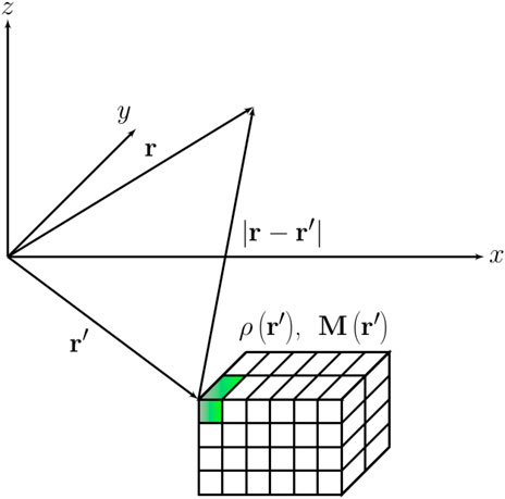
FIGURE 1. Illustration of the contribution to the potential $U\left(\mathbf{r}\right)$ associated with the three-dimensional distribution of monopolar $\left(\rho \left({\mathbf{r}}^{\prime }\right)\right)$ or dipolar $\left(\mathbf{M}\left({\mathbf{r}}^{\prime }\right)\right)$ sources.

For a finite volume V′, the total magnetic potential $V\left(\mathbf{r}\right)$ can be computed using the magnetization vector $\mathbf{M}\left({\mathbf{r}}^{\prime }\right)$ by:

$V\left(\mathbf{r}\right)=-\kappa {\iiint }_{V^{\prime }}\mathbf{M}\left({\mathbf{r}}^{\prime }\right)\cdot \nabla \left(\frac{1}{|\mathbf{r}-\mathbf{r}{|}^{\prime }}\right)d{v}^{\prime },(4)$

where κ = 4π × 10⁻⁷ H/m is the magnetic permeability of free space. Similar equations are also applicable to gradients of monopole fields including the gravity tensor.

It is important to note that all these fields depend on the relative position (e.g., Equations 3 and 4); these equations depend on a common factor that can be defined as a new function $W_0\left(\mathbf{r}\right)=\frac{1}{|\mathbf{r}|}$. This change of variable allows us to express Equations 3 and 4 in terms of three-dimensional convolution integrals, resulting in

$U\left(\mathbf{r}\right)=-{\gamma }_g\rho \left(\mathbf{r}\right)\ast W_0\left(\mathbf{r}\right),(5)$

for the gravity potential and

$V\left(\mathbf{r}\right)=-\kappa \mathbf{M}\left(\mathbf{r}\right)\cdot \ast \nabla \left(W_0\left(\mathbf{r}\right)\right),(6)$

for the magnetic potential, where ⋅∗ denotes 3D convolution $\left(\ast \right)$ for every inner product $\left(\cdot \right)$.

We can see that Equations 5 and 6 have the form of a convolution; this convolution can be solved for a finite volume using the appropriate W filter, computed by the field response of an individual prism for each depth layer.

In general, for a discretized volume divided in various layers of homogenous rectangular prisms with x − and y − regular dimensions (Figure 1), Equation 5 yields:

$U\left(x_l,y_m,z_n\right)={\gamma }_g\sum _i\sum _j\sum _k{\rho }_{ijk}{W}_k^D\left(x_l-x_i,y_m-y_j,z_n-z_k\right),(7)$

where $W_k^D\left(\alpha ,\beta ,\gamma \right)={\int }_{\alpha }^{\alpha +\mathrm{\Delta }x}{\int }_{\beta }^{\beta +\mathrm{\Delta }y}{\int }_{\gamma }^{\gamma +\mathrm{\Delta }{z}_k}\frac{1}{\sqrt{x^2+y^2+z^2}}dxdydz$. Using a discrete 2D convolution $\left(*\right)$ for a Δx, Δy equally spaced grid:

$U={\gamma }_g\sum _k{\rho }_k\ast W_k^D.(8)$

With this notation, we may compute g_z as:

$g_z=-{\gamma }_g\sum _k{\rho }_k\ast W_k^{g_z},(9)$

where $W_k^{g_z}=\frac{\partial W_k^D}{\partial z}$, i.e., (following Banerjee and Das Gupta, 1977)

$W_k^{g_z}\left(\alpha ,\beta ,\gamma \right)=\left[\alpha \ln \left(\beta +r\right)+\beta \ln \left(\alpha +r\right)-\gamma {\tan }^{-1}\left(\frac{\alpha \beta }{\gamma \rho }\right)\right]{|}_{\alpha }^{\alpha +\mathrm{\Delta }x}{|}_{\beta }^{\beta +\mathrm{\Delta }y}{|}_{\gamma }^{\gamma +\mathrm{\Delta }{z}_k}.(10)$

The gradient of the gravity field (gravity gradient tensor or GGT) contains the information of the vertical and horizontal gradients as well as the gravity field curvature (Jekeli, 2006); this means that it defines better lateral contrasts and discriminate depths and improves structural or geometrical indicators of the field (Butler, 1995). Similarly, we may compute the full GGT $\left(\mathbf{T}\right)$ as

$\mathbf{T}=-{\gamma }_g\sum _k{\rho }_k*W_k^T,(11)$

where $W_k^T=\nabla \nabla W_k^T\left(\alpha ,\beta ,\gamma \right)$, i.e.,

$W_k^T\left(\alpha ,\beta ,\gamma \right)=\left[\begin{array}{ccc}\hfill {\tan }^{-1}\left(\frac{\gamma \beta }{r\alpha }\right)\hfill & \hfill -\ln \left(r+\gamma \right)\hfill & \hfill -\ln \left(r+\beta \right)\hfill \\ \hfill -\ln \left(r+\gamma \right)\hfill & \hfill {\tan }^{-1}\left(\frac{\alpha \gamma }{r\beta }\right)\hfill & \hfill -\ln \left(r+\alpha \right)\hfill \\ \hfill -\ln \left(r+\beta \right)\hfill & \hfill -\ln \left(r+\alpha \right)\hfill & \hfill {\tan }^{-1}\left(\frac{\alpha \beta }{r\gamma }\right)\hfill \end{array}\right]{|}_{\alpha }^{\alpha +\mathrm{\Delta }x}{|}_{\beta }^{\beta +\mathrm{\Delta }y}{|}_{\gamma }^{\gamma +\mathrm{\Delta }{z}_k}.(12)$

We may also use the same function $\left(W_k^T\right)$ for the magnetic field as:

$\mathbf{B}=\kappa \sum _k{\mathbf{M}}_k\cdot \ast W_k^T.(13)$

The discrete convolution implies that if we have a fixed z position and a constant cell width, the derivative is the convolution of a characteristic 2D filter, which does not need to be evaluated individually. This allows for an efficient computation of sensitivities for thousands of observed data and horizontal cells. In fact, due to its symmetry, we only need to compute a single quadrant of the filter to cover the complete two-dimensional domain for each layer of cells (Figure 2), which can also be easily stored to avoid repeated computations when applying iterative procedures for inversion.

FIGURE 2

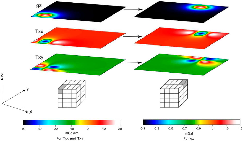
FIGURE 2. Illustration of convolution filters $\left(W_k\right)$ for the g_z, T_xx, and T_xy elements when acting on two shifted rectangular prisms located on the k − th layer of the model. Note that the anomalies result on a simple displacement in space.

2.2 Convolution-Based Conjugate Gradient Inversion

In order to solve the inverse problem, we use a quadratic norm to define the following objective function:

$\varphi =\Vert {\mathbf{d}}_{obs}-\mathbf{A}\mathbf{m}{\Vert }_{{\mathbf{C}}_{dd}^{-1}}^2+\Vert \mathbf{m}-{\mathbf{m}}_0{\Vert }_{{\mathbf{C}}_{00}^{-1}}^2+{\alpha }_p^2\Vert D\mathbf{m}{\Vert }^2,(14)$

where d_obs are the observed data, A is the sensitivity matrix, m accommodates all the model parameters (in our case either density or magnetization values per cell), C_dd is the covariance matrix of the observed data d_obs (assumed diagonal), C₀₀ is the covariance matrix of the a priori model m₀, and D is a discrete derivative operator that depends on the α_p penalty term and gears the search toward smoothed property distributions as a regularizing constraint. Am is the 3D model response that includes all the convolution coefficients indicated by Equations 9, 11, and 13.

We use a least-squares minimization, i.e., deriving (14) with respect to m and equating to zero for each component (Tarantola and Valette, 1982). We then obtain a linear system of equations for the optimal $\widehat{\mathbf{m}}$ estimator given by:

$\left({\mathbf{A}}^T{\mathbf{C}}_{dd}^{-1}\mathbf{A}+{\mathbf{C}}_{00}^{-1}+{\alpha }_p^2{\mathbf{D}}^T\mathbf{D}\right)\widehat{\mathbf{m}}={\mathbf{A}}^T{\mathbf{C}}_{dd}^{-1}{\mathbf{d}}_{obs}+{\mathbf{C}}_{00}^{-1}{\mathbf{m}}_0,(15)$

where T means transposed.

This system of linear equations can be solved using various linear algebra strategies. Direct solutions, however, may be prohibitive for large-scale three-dimensional problems, whereas the use of iterative schemes have to either face the repeated computation of the sensitivity matrix A or the storage of their compressed versions, usually at the cost of losing some resolution power.

To solve (15), we adapt the preconditioned conjugate gradient method (CG) described by Nocedal and Wright (2006) and take full advantage of the convolution property of the gravity and magnetic fields for an ensemble of equally sized cells. With this strategy, we avoid storing the sensitivity matrix or its Hessian and also the repetition of costly mathematical computations. As usual, preconditioners are recommended to reduce the number of iterations needed to solve the inversion problem.

To incorporate the convolution approach described in section 2.1, we modify the algorithm and illustrate the basic change using g_z as an example. The two main changes to incorporate the discrete convolution in the CG search are given as follows: 1) when computing the model response $\left(g=\mathbf{A}\mathbf{m}\right)$ and 2) when updating the search direction $\mathbf{r}=\mathbf{b}-{\mathbf{A}}^T{\mathbf{C}}_{dd}^{-1}\mathbf{A}$. They are computed as:

$g_{lm}=\sum _k\left[\sum _j\sum _i{\mathbf{m}}_{0ijk}{W}_{k\left(x_l-x_i,y_m-y_j\right)}^{g_z}\right],(16)$

and

${\mathbf{r}}_{\alpha ,\beta ,\gamma }={\mathbf{b}}_{\alpha ,\beta ,\gamma }-\left[\sum _l\sum _m\frac{g_{lm}}{{\sigma }_{lm}^2}\cdot W_{\gamma \left(\alpha -l,\beta -m\right)}^{g_z}\right].(17)$

We can see the full adaption of the algorithm in Table 1.

TABLE 1

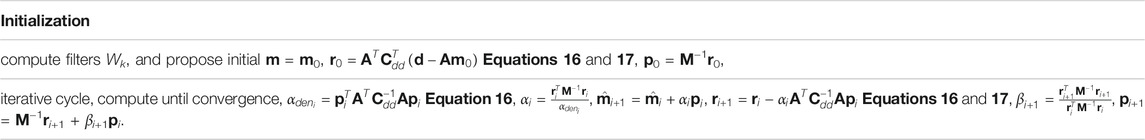
TABLE 1. Example of a M-preconditioned convolution-based conjugate gradient algorithm for the inversion of a set d data.

M-preconditioned convolution-based.

conjugate gradient algorithm to solve

$\left({\mathbf{A}}^T{\mathbf{C}}_{dd}^{-1}\mathbf{A}\right)\widehat{\mathbf{m}}={\mathbf{A}}^T{\mathbf{C}}_{dd}^{-1}\mathbf{d}$.

3 Synthetic Test Model

3.1 Test Model

We performed a rather conventional singular value decomposition (SVD) resolution analysis using the complete gravity tensor information to characterize exclusively the data sensitivity matrix. In this theory, a general rectangular m × n matrix A is factorized into two orthogonal vector basis U_m×n and V_n×n in the form

$\mathbf{A}={\mathbf{U}\mathbf{S}\mathbf{V}}^T,(18)$

where S_m×n is a partially diagonal matrix. With the aim of comparing the lateral and depth resolution of g_z and the six elements of GGT, the matrix A is analyzed for two cases: a) using g_z data along with the six elements of the gravity gradient tensor (GGT) and b) using only g_z.

Our synthetic model consists of a 2000, ×, 2000, ×, 1000 m volume discretized with 21 × 21 × 20 equally spaced rectangular prisms. Two density heterogeneities are formed with 3 × 3 × 3 elemental prims as shown in Figure 3. For the sole purpose of this sensitivity analysis, the A matrix is reassembled column by column using W filters as needed for each one of the 8,820 individual prisms that comprise the model.

FIGURE 3

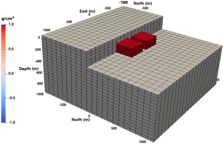
FIGURE 3. Three-dimensional configuration of the test density model. The model is composed of two anomalous rectangular prisms embedded in a homogenous and finite three-dimensional volume.

3.2 SVD Resolution Analysis

In this section, we only discuss the resolution analysis results in terms of the singular values S, leaving the singular vector (U and V) inspection in the appendix for the interested reader. As in conventional plots, the singular values are ordered from the highest to the lowest (Lanczos, 1996) and plotted in a log–log scale. Figure 4 shows the singular values normalized by the highest value for both g_z plus GGT data and g_z data alone cases.

FIGURE 4

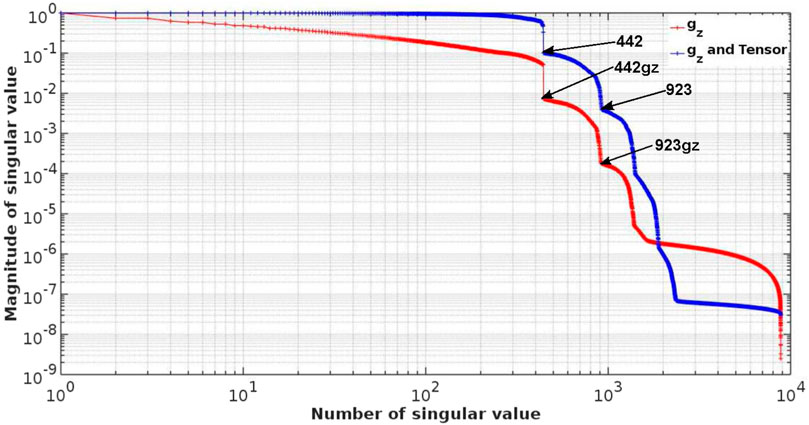
FIGURE 4. Singular values for the sensitivity matrix A when using only g_z (blue line) and with GGT (red line). Note the stepwise arrangement of the values and the faster decay of the g_z-computed values (in red).

For this plot, we may observe the following:

• Given both sets of singular values are normalized, it is clear that singular values when using only g_z decay faster than when adding GGT data. This accounts for the effective information supplied by the various forms of potential field data.

• For both cases, the decrease of the singular values becomes significant at discrete numbers. In this example, roughly every 441 element, which is the number of cells for each individual depth slice, indicating that resolution at depth decays faster when using a map of any potential field data.

• The magnitude of the sharp decreases at every 441 element is at least one order of magnitude: by example, the S₁ singular value for the sensitivity matrix of g_z and GGT together is 11.50 times greater than that of S₄₄₂ and 140.32 times greater than that of S₉₂₃; as comparison, for the first singular value of g_z alone, (S_gz1) is 136.19 times greater than S_gz442 and 5,571.42 times greater than S_gz923. This reflects a rapid loss of resolution when descending through each layer of the model.

3.3 Inversion Experiment

We use the synthetic model shown in Figure 3 to test the 3D inversion of synthetic gravimetric and magnetic data through our convolution-based CG method. Using this test model, we created synthetic data for both the vertical component of gravity g_z and the GGT and added normal random noise of 5% of the maximum value of the corresponding data type. This resulted in σ_dd = 0.01 mGal for g_z and σ_dd = 0.1 mGal/cm for all the components of the GGT data. Additionally, we start the inversion program with a density contrast of m₀ = 0.0 g/cm³, a standard deviation of the model σ₀₀ = 0.01 g/cm³, and a regularization parameter of α_p = 10.

The inversion process was stopped after 100 iterations, and the resulting model is shown in Figure 5. We note that when inverting only g_z data, the recovered density contrast values range between − 0.204 and 0.605 g/cm³, and the location of the largest positive contrast corresponds exactly to that of the heterogeneities of the original test model. The negative values accommodate around the recovered positive density contrast and may reflect the smoothed response when facing the original sharp contrast existent in the test model. As expected from the resolution analysis, the models bear a large smearing effect at depth when data resolution decreases.

FIGURE 5

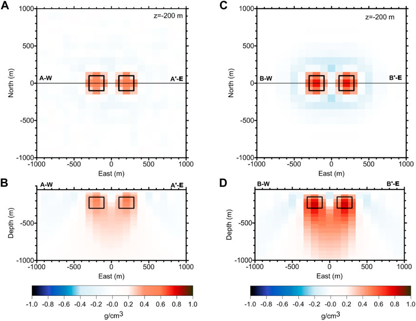
FIGURE 5. Plan (A) and vertical section (B) view of the recovered model after inversion of the gravity data in comparison to the plan (C) and vertical section (D) view of the model after inversion of g_z and GGT data. Outlined are the original borders of the test model heterogeneities.

We also note that when inverting GGT and g_z data together, the recovered density contrast values range between − 0.243 and 0.817 g/cm³, thus achieving a closer match to the values of the original test model heterogeneities. The distribution of these positive heterogeneities also depicts better the original boundaries of the test blocks and shows a reduced relative smearing at depth. In all these scenarios, the algorithm proves successful at retaining the expected resolution power in iterative schemes.

4 Field Data Experiment: Acoculco Geothermal Area

4.1 Geological Framework

The Acoculco caldera (AC) belongs to the Trans-Mexican Volcanic Belt (TMVB), the largest Neogene volcanic arc in North America with a length of almost 1000 km between 18°30′ and 21°30′ N in central Mexico, where volcanic activity is reported to have started about 16 Ma ago (Ferrari et al., 2012; Calcagno et al., 2018). The AC is located approximately 35 km southeast of the city of Pachuca, in the Mexican state of Hidalgo, in the eastern part of the TMVB. This caldera locates between the coordinates UTM 14 570 000 & 610,000 E and 2,190,000 & 2,220,000 N (López-Hernández et al., 2009); it has a semicircle shape and covers an area of ca. 40 × 30 km (Figure 6).

FIGURE 6

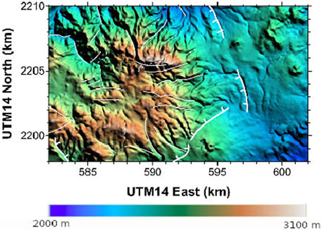
FIGURE 6. Digital elevation model of the Acoculco area and its geographical location. The solid lines indicate the major structural features identified in Avellán et al. (2019).

The AC is interesting for geothermal potential because of the presence of an extensive surface hydrothermal alteration, cold acid springs, and gas dischargers. Since 1981, the area has been analyzed by the Comision Federal de Electricidad (CFE) of Mexico that has drilled an exploratory well near Los Azufres with a depth of 2000 m in 1994, where stabilized temperatures rise above 300°C. The main objective of the well was to determine whether high temperatures and permeabilities existed at depth (López-Hernández et al., 2009). A second exploratory well (EAC-2) was drilled in 2008 with a depth of 1900 m and a maximum temperature of 264°C. None of the wells produced fluids; so, the zone is currently considered as a prospect to develop an enhanced geothermal system (EGS).

The caldera complex sits at the intersection of two regional fault systems with NE–SW and NW–SE orientations. A NE–SW alignment of volcanic cones and medium-sized composite volcanoes can be observed. These volcanoes could be related to the NE-striking Apan–Piedras Encimadas Lineament (López-Hernández et al., 2009; Calcagno et al., 2018). The NW–SE-trending fault system is represented by subtle morphological lineaments between the Pachuca and Apan regions, NW of the Acoculco zone (López-Hernández et al., 2009). The AC was built atop Cretaceous limestones, the Zacatán basaltic plateau of unknown age, early Miocene domes ($\sim 12.7-10.98Ma$), and Pliocene ($\sim 3.9,-,3Ma$) lava domes (Avellán et al., 2020).

The oldest outcropping rocks are located in the eastern area and correspond to Cretaceous sedimentary rocks from the Sierra Madre Oriental. These rocks cannot be found in other zones inside the region; nevertheless, various exploratory wells in the AC show their existence at depth. These rocks are affected for various calco-alkaline events, which occurred in most of the area, resulting in several sequences of volcaniclastic deposits, lava flows, and intrusives. The existing igneous materials vary both in their composition (from basaltic to rhyolitic) and their structural arrangement, making the area a difficult target of exploration (López-Hernández et al., 2009).

According to López-Hernández et al. (2009), the stratigraphic sequence of the Tulancingo–Acoculco complex can be described from the exploratory well EAC-1 with the following lithology (from bottom to top): 340 m of an intrusive body who is responsible for metamorphism of the boxing rock, 870 m of an intensely metamorphosed sedimentary sequence (skarn), and 790 m of a volcanic sequence related with the activity of the complex.

4.2 Gravity Data Inversion

The analyzed area inside the AC is located between the coordinates UTM 14 582 000 & 602,000 E and 2,198,000 & 2,210,000 N covering an area of 20 × 12 km; the gravity data were collected in stations located through existing roads and highways in the area, to make a network of stations distributed in the form of polygons with a mean diameter of 5 km and measurement points separated every 250 m (Figure 7). The measurements were made using Worden Master (Texas Instruments) gravity meters with an accuracy of tenths of μGal (López-Hernández et al., 2009).

FIGURE 7

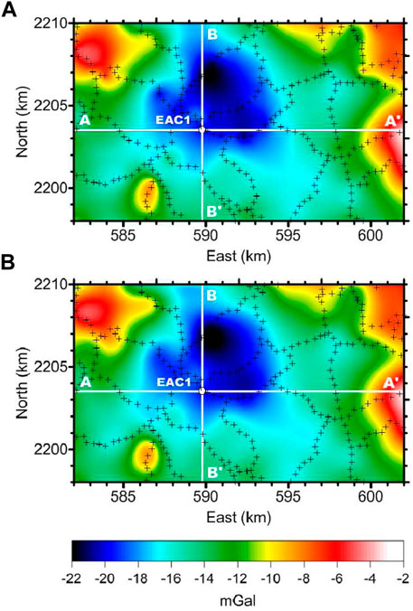
FIGURE 7. Observed (A) and computed (B) residual gravity response for the studied area. Note the resemblance of the major and local features and the overall match of the main geological lineaments (Figure 6). The stations of collected data are shown as black cross; the white solid lines indicate the location of the shown sections of the estimated three-dimensional density contrast model. EAC-1 corresponds to the exploratory borehole.

The Bouguer anomaly data were re-sampled on a grid spaced 200 m and processed to obtain a regular grid for analysis. A linear regional trend using the values at the ends of the map was removed to capture the gravimetric effect of the overlying material to basement. The gravity values were shifted to produce a residual negative gravity anomaly suitable for inversion (Figure 7). We see that the minimum gravity value locates near the center of the studied map and forms a semicircular structure located north of the borehole EAC-1. This negative gravity anomaly extends, with lower intensities, in the preferential regional directions (NW–SE and NE–SW). The maximum gravity values are located to the NE and NW of the studied area denoting a decreased vulcanosedimentary thickness.

The Acoculco density model was composed of a 20 × 12 km volume using 101 × 61 × 100 equally sized (200m × 200m × 30m) rectangular prisms. We assigned a standard deviation for the observed data of σ_dd = 0.01 mGal.

Our program starts with an initial model m_ini = 0.0 g/cm³ and was stopped when the rms reached a value less than 2% with respect to the maximum gravity value; the average time of the iterations was of 458.35 s compared with the 1,250.1 s of the computation time of the matrix A. The model response is displayed in Figure 7.

The estimated density contrast model is shown in Figure 8. For the deepest model slice (2,800 m), it becomes clear that the high-density contrast material surrounds (E, NE, NW, and SW) the less dense material to the north of borehole EAC-1, which goes in agreement with the overall structural caldera. There are, however, clear preferential directions of the less dense materials (NW–SE, NE–SW, E–W, and N–S), which agrees with the known regional tectonic scenario. These features also imprint in the shallower depth slice shown in Figure 8B, which indicates the action of the normal smearing of the model at depth. This depth smearing is confirmed by the selected vertical sections included in Figure 8.

FIGURE 8

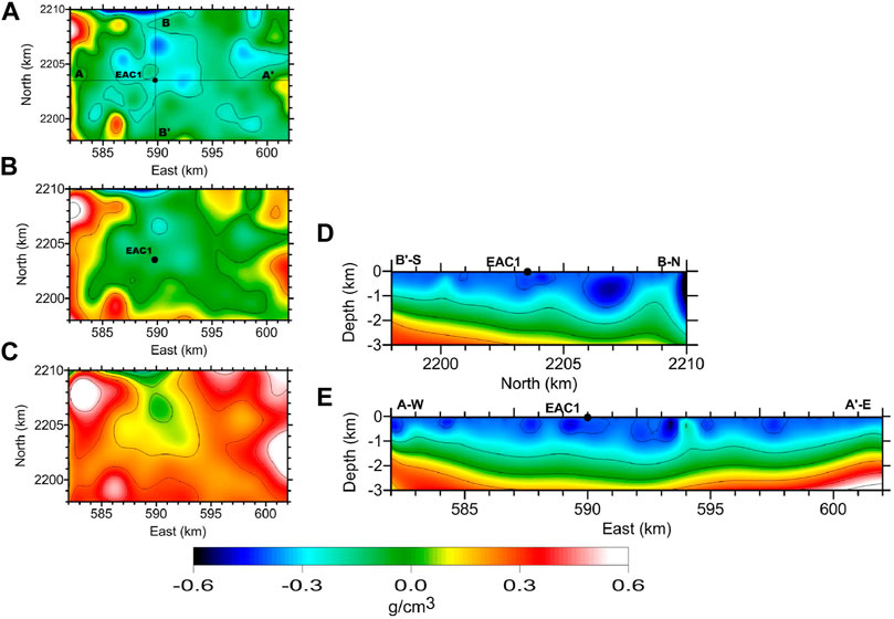
FIGURE 8. Selected horizontal slices at depths (A) 1,500 m, (B) 2000 m, and (C) 2,800 m and vertical sections (D) S-N and (E) E-W of the estimated density contrast model for the selected Acoculco area.

The shallowest model slice (Figure 8A) is almost completely dominated by low-density contrast materials that more likely belong to the upper vulcanosedimentary sequence that fill in the structural crater left by the various calderic episodes.

Figures 8D,E are vertical sections, which mainly denote the varied thicknesses of the vulcanosedimentary cover.

4.3 Magnetic Data Inversion

As in the case of the gravimetric data, the area of the AC for the magnetic data is between the coordinates UTM 14 582 000 & 602,000 E and 2,198,000 & 2,210,000 N. The aeromagnetic total magnetic field (TMI) data were provided by the Servicio Geologico Mexicano for the Acoculco area. The distance among flight lines was 1 km with direction N–S; the E–W control lines are 5 km separated, and the flight height was 300 m above ground level. The data were processed with MagMap tools in Oasis Montaj^® to produce the 200 m-spaced reduced-to-the-pole (RTP) anomaly map used for inversion (Figure 9).

FIGURE 9

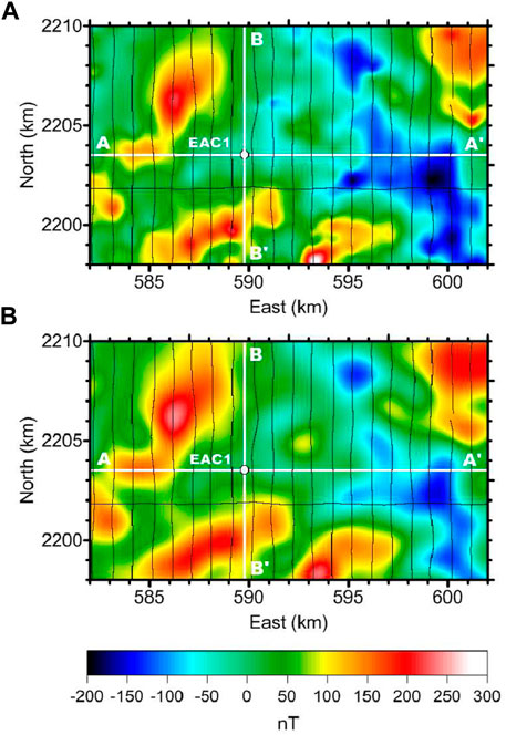
FIGURE 9. Observed (A) and computed (B) reduced to pole magnetic anomaly for the studied area. Note the resemblance of the major and local features and the overall match of the main geological lineaments (Figure 6). The flight lines are shown in black solid lines; the white solid lines indicate the location of the shown sections of the estimated three-dimensional density model. EAC-1 corresponds to the exploratory borehole.

To perform the RTP data inversion from Acoculco and maintain a magnetization contrast model consistent to the previous density model for Acoculco, we used a magnetization contrast model with exactly the same dimensions and spacing to that used for the density contrast model. We then assumed a standard deviation to the observed RTP data of 0.1 nT and started the process with an initial model of m_ini = 0.0 A/m. The program stopped at the 100th iteration taking an average time per iteration of 450.98 s. The model reached an acceptable normalized data misfit (rms = 3.34), and their data response is shown in Figure 9B.

Figure 10 shows various slices of the resulting magnetization contrast model. At the deepest horizontal slice, at 2,800 m depth below ground, we can observe several major magnetization contrast zones with trends in different directions. The largest zone with minimum magnetization contrast intensities orients NW–SE. This zone is flanked east by a narrower zone with large magnetization contrast. The borehole EAC-1 locates exactly between two of these positive magnetization contrast zones.

FIGURE 10

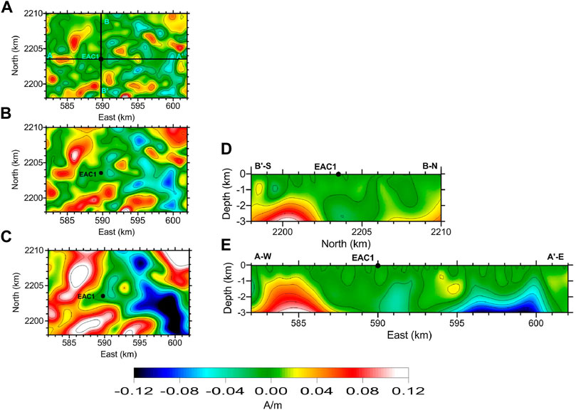
FIGURE 10. Selected horizontal slices at depths (A) 1,500 m, (B) 2000 m, and (C) 2,800 m and vertical sections (D) S-N and (E) E-W of the magnetization contrast model for the Acoculco area.

At 2000 m depth (Figure 10B), the largest negatively magnetized heterogeneity trending NE–SW and the positive magnetization contrast volume shown at the largest depth remain but are narrower; in the north-east corner, a positive magnetization contrast region with trend NW–SE is found. All these anomalous volumes are subdivided in smaller regions depicting an increased geological heterogeneity. At 1,500 m depth (Figure 10A), we observe several isolated volumes with local positive or negative magnetization contrast. The borehole EAC-1 is flanked NE–SW by two local negative magnetization contrast regions.

The EW section (Figure 10D) evidences the continuity at depth of the positive (west) and negative (east) magnetization contrast heterogeneities. These regions are overlain by several local magnetization contrast areas. Differently, the S–N section (Figure 10E) shows two deeper high-magnetization contrast volumes flanking the low-magnetization contrast heterogeneity around the borehole EAC-1.

5 Integrated Interpretation

The resulting 3D distributions of density contrast (Figure 8) and magnetization contrast (Figure 10) are somewhat limited in resolution. This is a natural consequence of the divergent decay of both potential fields reflected not only at depth but also laterally due to the separation of the original aeromagnetic flight lines and the sparsity of the actual gravity stations. Nevertheless, there are several geological features that can be confidently inferred from the interpreted models. From the point of view of the density contrast model of Figure 8, the clearest feature to identify corresponds to the distribution of the volcanosedimentary infill in the area, which is delimited by the shallow largest negative density contrast. Differently, the magnetization contrast distribution depicts various located units of both magnetic and non-magnetic materials, most of them inferred at basement depths that may be originated by various intrusive events.

In general, we may identify at least four units, which clearly match the reported lithological groups in their stratigraphic and structural disposition (see, for e.g., López-Hernández et al., 2009; Avellán et al., 2020). They include (see Figure 11):

Unit I. A low-density contrast zone with various magnetization contrast values. These combined values imply unconsolidated materials with a range of mineralogical compositions. These materials correlate with the alluvial and volcaniclastic deposits with a low level of compaction that came to occupy the large caldera structure.

Unit II. A zone with high-density contrast and high-positive magnetization contrast. This unit may correlate to various intrusions dominated by ferromagnetic compositions as reported in the late events of the volcanic sequences of the area (cf. Sosa-Ceballos et al., 2018; Avellán et al., 2020).

Unit III. A zone with high-density contrast and high-negative magnetization contrast. This zone may correspond to non-magnetic intrusions. According to the apparent intrusion sequence, these intrusions precede the magnetic intrusions of Unit II, since it is intersected by them at various locations.

Unit IV. A high-density contrast and null magnetization contrast zone. This unit matches the position of the cretaceous limestone that conforms to the regional basement in the area. This basement is largely intruded by units II and III.

FIGURE 11

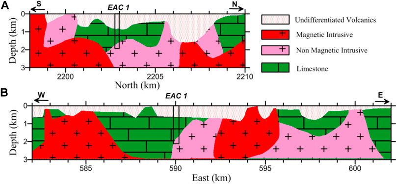
FIGURE 11. Interpreted south–north (A) and east–west (B) sections for the Acoculco area. Selection of lithologies is based on the combined values of density and magnetization contrasts of the inverted model (Figures 8, 10). Note that the distinction between the proposed intrusives is mainly based on their differences in magnetization contrast.

The structure of the caldera is noticeable in Figure 8A by the lower density contrast of the deposits that came to fill the formed topographic depression. Differently, the basement shows an evident structural control, having dominant non-magnetic intrusives (Unit III) along a preferable trend NW–SE which runs along the east of the mapped volume. One of these intrusives seems to correspond to the hornblende granite reached by the exploratory well EAC-1 (López-Hernández et al., 2009). The intrusives of the more ferromagnetic composition occur in various events aligned in a preferential SW–NE direction (Figure 10) and are likely to be associated with the latest events of magmatism in the area that resulted in several basalt-dominant deposits of more recent age (Avellán et al., 2020). Both alignments are clearly associated with more regional lineaments identified in the larger extension of the TMVB (see, for e.g., Avellán et al., 2019).

From a geothermal potential point of view, it seems clear that the area around the exploratory well EAC-1 is largely extended in between Cretaceous limestone and the various intrusives which are naturally highly impermeable rocks. The evidence of high temperature in the well, however, indicates the influence of a nearby heat source. Considering the various potential ages of the intrusive events and the closeness of the intrusive of Unit II to EAC-1, it seems very likely that this material or their younger magmatic feed may be responsible of both fracture motivation and heat transfer as suggested by Sosa-Ceballos et al. (2018). In this scenario, the mapped flanks of this Unit II may be a suitable place to explore temperature potential to evaluate the feasibility of developing an enhanced geothermal system. It is noted that this high temperature evidence only occurs at depth in the well surroundings and does not seem to be correlated to the shallower basin of the caldera filled with volcanic deposits that may conform to upper aquifers for the zone.

6 Conclusion

We have developed a convolution-based conjugate gradient algorithm for the inversion of potential field data to produce three-dimensional volumes of density or magnetization contrasts. The algorithm computes exact convolutional filters that permit the storage of a highly compressed but exact sensitivity matrix. By using regular data grids and models, the convolution prevents not only the repeated computation of costly mathematical instructions but also the use of interpolated values from the filters.

Using singular value decomposition and a synthetic test, we show that the proposed methodology bears neither loss of data information nor model resolution achieving highly detailed inversion models in small computational infrastructures.

We prove the algorithms applicability on the Acoculco geothermal area in Mexico, where we successfully inverted land gravity and aeromagnetic data. From the combined density and magnetization contrasts values and the lithological information provided by an exploratory well, we could distinguish a group of intrusive bodies at depth as potential low-permeability geothermal reservoirs and their interaction with younger intrusive bodies as potential heat sources. We found no apparent connection of the deep basement with the volcanosedimentary cover and thus no direct connection with local aquifers in the area. The combined models yielded a coherent interpretation of a complicated volcanic caldera and helped to elucidate their implications for the development of an actual enhanced geothermal system.

Data Availability Statement

The data analyzed in this study is subjected to the following licenses/restrictions: private data for copyright. Requests to access these data sets should be directed to lgallard@cicese.mx.

Author Contributions

JC contributed to investigation, conceptualization, methodology, visualization, and writing–original draft. LG contributed to conceptualization, methodology, supervision, resources, and writing–review and editing.

Funding

The research was partially funded by the GEMex project. (Conacyt-Sener #268074; Horizon 2020 #727550).

Conflict of Interest

The authors declare that the research was conducted in the absence of any commercial or financial relationships that could be construed as a potential conflict of interest.

Publisher’s Note

All claims expressed in this article are solely those of the authors and do not necessarily represent those of their affiliated organizations, or those of the publisher, the editors, and the reviewers. Any product that may be evaluated in this article, or claim that may be made by its manufacturer, is not guaranteed or endorsed by the publisher.

Acknowledgments

The authors appreciate supporting funding for this research from the GEMex project (Conacyt-Sener #268074; Horizon 2020 #727550). JC thanks CONACYT for the scholarship awarded during the doctoral period at CICESE.

References

Aleshin, I. M., Soloviev, A. A., Aleshin, M. I., Sidorov, R. V., Solovieva, E. N., and Kholodkov, K. I. (2020). Prospects of Using Unmanned Aerial Vehicles in Geomagnetic Surveys. Seism. Instr. 56, 522–530. doi:10.3103/s0747923920050059

CrossRef Full Text | Google Scholar

Ascher, U. M., and Haber, E. (2001). Grid Refinement and Scaling for Distributed Parameter Estimation Problems. Inverse Probl. 17, 571–590. doi:10.1088/0266-5611/17/3/314

CrossRef Full Text | Google Scholar

Avellán, D. R., Macías, J. L., Layer, P. W., Cisneros, G., Sánchez-Núñez, J. M., Gómez-Vasconcelos, M. G., et al. (2019). Geology of the Late Pliocene–Pleistocene Acoculco Caldera Complex, Eastern Trans-mexican Volcanic belt (México). J. Maps 15, 8–18. doi:10.1080/17445647.2018.1531075

CrossRef Full Text | Google Scholar

Avellán, D. R., Macías, J. L., Layer, P. W., Sosa-Ceballos, G., Gómez-Vasconcelos, M. G., Cisneros-Máximo, G., et al. (2020). Eruptive Chronology of the Acoculco Caldera Complex–A Resurgent Caldera in the Eastern Trans-mexican Volcanic belt (México). J. South Am. Earth Sci. 98, 102412. doi:10.1016/j.jsames.2019.102412

CrossRef Full Text | Google Scholar

Banerjee, B., and Das Gupta, S. P. (1977). Gravitational Attraction of a Rectangular Parallelepiped. Geophysics 42, 1053–1055. doi:10.1190/1.1440766

CrossRef Full Text | Google Scholar

Blakely, R. J. (1996). Potential Theory in Gravity and Magnetic Applications. New York: Cambridge University Press.

Google Scholar

Butler, D. K. (1995). Generalized Gravity Gradient Analysis for 2-d Inversion. Geophysics 60, 1018–1028. doi:10.1190/1.1443830

CrossRef Full Text | Google Scholar

Calcagno, P., Evanno, G., Trumpy, E., Gutiérrez-Negrín, L. C., Macías, J. L., Carrasco-Núñez, G., et al. (2018). Preliminary 3-D Geological Models of Los Humeros and Acoculco Geothermal fields (Mexico) - H2020 GEMex Project. Adv. Geosci. 45, 321–333. doi:10.5194/adgeo-45-321-2018

CrossRef Full Text | Google Scholar

Caratori Tontini, F., Cocchi, L., and Carmisciano, C. (2009). Rapid 3-d Forward Model of Potential fields with Application to the Palinuro Seamount Magnetic Anomaly (Southern Tyrrhenian Sea, italy). J. Geophys. Res. Solid Earth 114, B02103. doi:10.1029/2008jb005907

CrossRef Full Text | Google Scholar

Chen, L., and Liu, L. (2019). Fast and Accurate Forward Modelling of Gravity Field Using Prismatic Grids. Geophys. J. Int. 216, 1062–1071. doi:10.1093/gji/ggy480

CrossRef Full Text | Google Scholar

Cuer, M., and Bayer, R. (1980). Fortran Routines for Linear Inverse Problems. Geophysics 45, 1706–1719. doi:10.1190/1.1441062

CrossRef Full Text | Google Scholar

Davis, K., and Li, Y. (2011). Fast Solution of Geophysical Inversion Using Adaptive Mesh, Space-Filling Curves and Wavelet Compression. Geophys. J. Int. 185, 157–166. doi:10.1111/j.1365-246x.2011.04929.x

CrossRef Full Text | Google Scholar

Dransfield, M., and Zeng, Y. (2009). Airborne Gravity Gradiometry: Terrain Corrections and Elevation Error. Geophysics 74, I37–I42. doi:10.1190/1.3170688

CrossRef Full Text | Google Scholar

Ferrari, L., Orozco-Esquivel, T., Manea, V., and Manea, M. (2012). The Dynamic History of the Trans-mexican Volcanic belt and the mexico Subduction Zone. Tectonophysics 522-523, 122–149. doi:10.1016/j.tecto.2011.09.018

CrossRef Full Text | Google Scholar

Jekeli, C. (2006). Airborne Gradiometry Error Analysis. Surv. Geophys. 27, 257–275. doi:10.1007/s10712-005-3826-4

CrossRef Full Text | Google Scholar

Jiang, D., Zeng, Z., Zhou, S., Guan, Y., and Lin, T. (2020). Integration of an Aeromagnetic Measurement System Based on an Unmanned Aerial Vehicle Platform and its Application in the Exploration of the Ma'anshan Magnetite Deposit. IEEE Access 8, 189576–189586. doi:10.1109/access.2020.3031395

CrossRef Full Text | Google Scholar

Lanczos, C. (1996). Linear Differential Operators. Philadelphia: SIAM.

Google Scholar

Li, X., and Chouteau, M. (1998). Three-dimensional Gravity Modeling in All Space. Surv. Geophys. 19, 339–368. doi:10.1023/a:1006554408567

CrossRef Full Text | Google Scholar

Li, Y., and Oldenburg, D. W. (2003). Fast Inversion of Large-Scale Magnetic Data Using Wavelet Transforms and a Logarithmic Barrier Method. Geophys. J. Int. 152, 251–265. doi:10.1046/j.1365-246x.2003.01766.x

CrossRef Full Text | Google Scholar

López-Hernández, A., García-Estrada, G., Aguirre-Díaz, G., González-Partida, E., Palma-Guzmán, H., and Quijano-León, J. L. (2009). Hydrothermal Activity in the Tulancingo-Acoculco Caldera Complex, central mexico: Exploratory Studies. Geothermics 38, 279–293. doi:10.1016/j.geothermics.2009.05.001

CrossRef Full Text | Google Scholar

Martin, R., Monteiller, V., Komatitsch, D., Perrouty, S., Jessell, M., Bonvalot, S., et al. (2013). Gravity Inversion Using Wavelet-Based Compression on Parallel Hybrid Cpu/gpu Systems: Application to Southwest ghana. Geophys. J. Int. 195, 1594–1619. doi:10.1093/gji/ggt334

CrossRef Full Text | Google Scholar

Moorkamp, M., Jegen, M., Roberts, A., and Hobbs, R. (2010). Massively Parallel Forward Modeling of Scalar and Tensor Gravimetry Data. Comput. Geosci. 36, 680–686. doi:10.1016/j.cageo.2009.09.018

CrossRef Full Text | Google Scholar

Mottl, J., and Mottlová, L. (1972). Solution of the Inverse Gravimetric Problem With the Aid of Integer Linear Programming. Geoexploration 10, 53–62. doi:10.1016/0016-7142(72)90013-0

CrossRef Full Text | Google Scholar

Nabighian, M. N., Ander, M. E., Grauch, V. J. S., Hansen, R. O., LaFehr, T. R., Li, Y., et al. (2005). Historical Development of the Gravity Method in Exploration. Geophysics 70, 63ND–89ND. doi:10.1190/1.2133785

CrossRef Full Text | Google Scholar

Nocedal, J., and Wright, S. (2006). Numerical Optimization. New York: Springer Science & Business Media.

Google Scholar

Parker, R. L., and Huestis, S. P. (1974). The Inversion of Magnetic Anomalies in the Presence of Topography. J. Geophys. Res. 79, 1587–1593. doi:10.1029/jb079i011p01587

CrossRef Full Text | Google Scholar

Parshin, A. V., Budyak, A. E., and Babyak, V. N. (2020). Interpretation of Integrated Aerial Geophysical Surveys by Unmanned Aerial Vehicles in Mining: a Case of Additional Flank Exploration. IOP Conf. Ser. Earth Environ. Sci. 459, 052079. doi:10.1088/1755-1315/459/5/052079

CrossRef Full Text | Google Scholar

Pilkington, M. (1997). 3-d Magnetic Imaging Using Conjugate Gradients. Geophysics 62, 1132–1142. doi:10.1190/1.1444214

CrossRef Full Text | Google Scholar

Safon, C., Vasseur, G., and Cuer, M. (1977). Some Applications of Linear Programming to the Inverse Gravity Problem. Geophysics 42, 1215–1229. doi:10.1190/1.1440786

CrossRef Full Text | Google Scholar

Shin, Y. H., Choi, K. S., and Xu, H. (2006). Three-dimensional Forward and Inverse Models for Gravity fields Based on the Fast Fourier Transform. Comput. Geosci. 32, 727–738. doi:10.1016/j.cageo.2005.10.002

CrossRef Full Text | Google Scholar

Sorokin, L. (1951). Gravimetry and Gravimetrical Prospecting. Moscow: State Technology Publising. in Russian.

Google Scholar

Sosa-Ceballos, G., Macías, J. L., Avellán, D. R., Salazar-Hermenegildo, N., Boijseauneau-López, M. E., and Pérez-Orozco, J. D. (2018). The Acoculco Caldera Complex Magmas: Genesis, Evolution and Relation with the Acoculco Geothermal System. J. Volcanol. Geothermal Res. 358, 288–306. doi:10.1016/j.jvolgeores.2018.06.002

CrossRef Full Text | Google Scholar

Sun, S.-Y., Yin, C.-C., Gao, X.-H., Liu, Y.-H., and Ren, X.-Y. (2018). Gravity Compression Forward Modeling and Multiscale Inversion Based on Wavelet Transform. Appl. Geophys. 15, 342–352. doi:10.1007/s11770-018-0676-7

CrossRef Full Text | Google Scholar

Tarantola, A., and Valette, B. (1982). Generalized Nonlinear Inverse Problems Solved Using the Least Squares Criterion. Rev. Geophys. 20, 219–232. doi:10.1029/rg020i002p00219

CrossRef Full Text | Google Scholar

Walter, C., Braun, A., and Fotopoulos, G. (2020). High‐resolution Unmanned Aerial Vehicle Aeromagnetic Surveys for mineral Exploration Targets. Geophys. Prospecting 68, 334–349. doi:10.1111/1365-2478.12914

CrossRef Full Text | Google Scholar

Zhdanov, M. S., Ellis, R., and Mukherjee, S. (2004). Three‐dimensional Regularized Focusing Inversion of Gravity Gradient Tensor Component Data. Geophysics 69, 925–937. doi:10.1190/1.1778236

CrossRef Full Text | Google Scholar

Appendix: SVD for Singular Vectors

Analysis of Singular Vectors U and Data Information

Selected singular vectors U of the SVD of the sensitivity matrix A (Equations 10 and 12) are shown in Figure 12. The images show a comparison of both data group scenarios toward reproducing any g_z anomaly: with g_z alone (at the left column) and with g_z and GGT (at the right column).

FIGURE 12

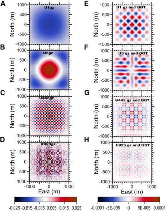
FIGURE 12. Comparison of the g_z components of the singular vector U when using only g_z (left column) and GGT plus g_z data (right column) for the following ordered singular value numbers: 1 (A,E), 5 (B,F), 442 (C,G), and 923 (D,H).

The general characteristics for the vectors of the matrix U are:

• The vector U₁ is the first information used by the algorithm to recover an anomaly.

• The first vectors anomalies have a wavelength equal to the size of the corresponding cell.

• The anomalies contribution direction depends of the gradient direction.

• The left matrix U represents the type of anomalies which would be necessary to activate the corresponding singular value, i.e., the first to be used during the inversion process.

A general remark for both columns is that when using only g_z data, the dominant information is provided by the overall domain, thus concentrating on the long wavelength anomaly, which in practical inversion problems, is likely to be reflected as border problems. After this border effect, the information decays rapidly for the singular vectors associated with smaller singular values, indicating a rapid loss of information extractable from the anomaly. Both effects are significantly reduced when using combined potential field data, which enables a more continuous use of information from the first singular vectors and continues gradually to vectors associated with smaller singular values.

Analysis of Singular Vectors V and Model Resolution

Selected singular vectors V (V₁, V₅, V₄₂₂, and V₉₂₃) are shown in Figure 13 when using g_z and GTT data combinedly. For V₁, it is noticeable that the intensity of the values is higher in the center of the top layer; this suggests that they are the first prisms to be resolved during inversion without taking much into account the lower layers. For vector V₅, we observe that it is only sensitive to upper layers; however, the intensities of the central prisms begin to decrease, leaving resolution capabilities to other cells of the upper layer of the model. Vectors V₄₂₂ and V₉₂₂ indicate that after using the first layers of information, the sensitivity matrix can effectively start solving intermediate layers more directly.

FIGURE 13

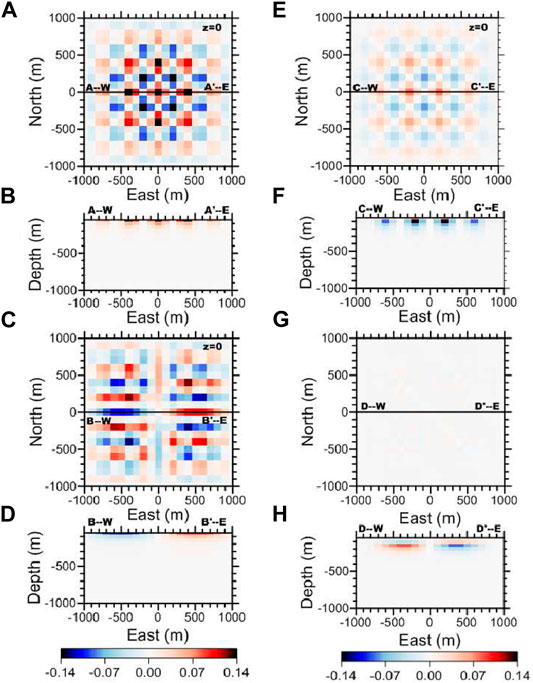
FIGURE 13. Illustration of selected V singular vectors of the matrix A when using g_z and GGT combinedly. (A) Horizontal and (B) vertical sections of V₁, (C) horizontal and (D) vertical sections of V₅, (E) horizontal and (F) vertical sections of V₄₂₂, and (G) horizontal and (H) vertical sections of V₉₂₂.