Using the Residual Network Module to Correct the Sub-Seasonal High Temperature Forecast

1 Introduction

Most of the existing high temperature forecasts are short term, with forecasts of a few hours to a few days with no time to prepare more adequately for extreme weather. Therefore, the establishment of forecasting models with longer extension periods meets the public’s need for longer lead times. Such models will provide early warnings of extreme weather that may come, making it easier for people to prepare in advance. The sub-season, a time scale between weather and seasons, soon entered the limelight. As early as 2010, the World Weather Research Programme (WWRP) and the World Climate Research Programme (WCRP) identified the need for in-depth research on the sub-seasonal to seasonal (S2S) scale to improve the prediction of extreme weather events, such as droughts, floods, and cyclones (Brunet et al., 2010). As the research continues, researchers have repeatedly argued the value of sub-seasonal forecasting studies as a key component of completing seamless forecasts (Pegion et al., 2019; Xiang et al., 2019; Phakula et al., 2020; Vijverberg et al., 2020; Manrique-Sun˜e´n et al., 2020; Merryfield et al., 2020). However, this timescale is hard to forecast due to the fact that the lead time is sufficiently long that the memory of the atmospheric initial conditions is lost and it is too short a time range for the variability of the ocean to have a strong influence on the atmosphere. Researchers have tried to study it through Kalman filtering and integrated models (Zhu, 2005; Gel, 2007; Durai and Bhradwaj, 2014). Although some results have been achieved, the high maintenance and development costs of the models and the large deviations in some areas, such as mountainous areas, have been difficult to solve.

The advent of artificial intelligence now provides a very different approach to alleviate these problems, with greater flexibility in extracting relationships in the data and building forecast models for target areas. In the field of deterministic forecasting, with this technology, researchers have made good progress in proposing several artificial intelligence models for sub-seasonal studies, showing that the application of these methods in the field of sub-seasonal forecasting is feasible (Cohen et al., 2019; Hwang et al., 2019; He et al., 2020). In 2019, researchers corrected and analyzed the systematic errors of sub-seasonal forecasts from the U.S. National Weather Center, and the experiments showed that the accuracy of the corrected forecasts was improved significantly. This provides a new idea for sub-seasonal-scale forecasting: error correction of existing forecasts (Guan et al., 2019). To implement this idea, we select hindcast data from the ECMWF (Son et al., 2020), which reflects sub-seasonal characteristics, and correct it for systematic errors over a 30-day period. To build a complete set of forecasting system from deterministic to probabilistic forecast, we focus on probabilistic forecasting at sub-seasonal scales. In the sub-seasonal domain, the integrated probabilistic model (Vigaud et al., 2019) and the machine learning (Peng et al., 2020) model achieve good results. After reflecting on the previous studies, we establish the connection between it and the probability distribution based on the error correction results in deterministic forecasts, and finally, build probabilistic forecast models for the next 30 days at the sub-seasonal scale. Unlike traditional methods and machine learning approaches, we used convolutional networks to consider interactions between grids, drawing on residual structures that have been successful in computer vision to complete the design of the model details. Ultimately, we tested and analyzed them.

2 Data, Models, and Other Details

2.1 Data Processing

To research the forecast of sub-seasonal high temperature, we use two datasets at a resolution of 1.5°×1.5°. One is the hindcast data of the maximum temperature at 2 m from ECMWF with four versions (2015, 2016, 2017, and 2018) from 1995 to 2014 and the other is 2-m temperature daily observation data by natural neighborhood interpolation from more than 2,400 stations in China. Our study area is part of China with a spatial range of 19.5°N–45°N and 105°E–132°E.

The European hindcast data uses the Universal Time and a six-hourly forecast cycle. To match the data to be input to the network with the observations, we convert the European hindcast data to Beijing time and reselect the maximum of four consecutive sets of forecasts as the hindcast high temperature data for the day of the observation. As is well-known, the European hindcast data contains eleven ensemble members which are represented below by “channel”: one control forecast and ten perturbed forecasts. Following the temporal treatment described earlier, for each forecast, it will correspond to eleven unordered high temperature data. We artificially specify their arrangement rules: the eleven unordered data are arranged in ascending order, and the same forecast days are selected from the different starting time to generate 30 different forecast day datasets, respectively, named eleven channel datasets. In Table 1, 0 to 10 is the sequence numbers after channel sorting. We take equal spacing to select channels to filter the dataset with six different channel numbers of 1, 2, 3, 4, 5, and 11. A checkmark indicates that the dataset contains the channel at that sequence. To verify the excellence of the eleven channel data, we performed regular channel selection according to Table 1 and generate five datasets with the different number of channels to compare the effect of various datasets. In addition, we use the ensemble mean of eleven channel data as a forecast baseline for European hindcast data.

TABLE 1

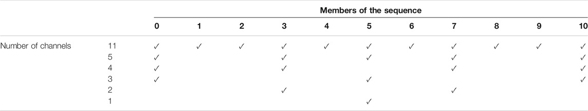
TABLE 1. Multi-dataset channel selection.

In Table 2, the testing results for different datasets are listed and five forecast days (2nd, 9th, 16th, 23rd, and 30th) are chosen as test subjects to compare the errors of the six datasets in the case of three residual modules (the experiments are like Section 3.1). LF and EI denote loss function and evaluation index, respectively. It can be noticed that the error decreases with the number of channels until it reaches a minimum at the eleven-channel dataset bolded in the table. This indicates that unnecessary filtering channels can lose some hidden feature information and, thus, reduce the prediction performance of the model, so the eleven-channel dataset is the best choice for the experiments.

TABLE 2

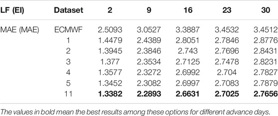
TABLE 2. Multi-channel dataset filtering results.

2.2 Framework and Model

As shown in Figure 1A, the proposed overall framework consists of two modules: a deterministic forecast module (red box) and a probabilistic forecast module (blue box). In the deterministic forecast module, the data of eleven channels as the input feed the trained network with Parameter 1 to obtain the revised forecast data. It is known that the high temperature probability satisfies the Gaussian distribution. To strengthen the connection between the deterministic module and the probabilistic forecast module, the output of the deterministic prediction module is taken as the input of the probabilistic forecast module and becomes the expectation of the probability distribution. The same network with Parameter 2 has been trained to obtain the corresponding standard deviation of the distribution. Finally, the expectation and the standard deviation are substituted into the Gaussian probability distribution formula to get the probability needed. The network structure of the deterministic forecast and the probabilistic forecast is the same on the same forecast day. Only the numbers of residual modules are the same, but the parameters are different, so they are denoted as Parameter 1 and Parameter 2, respectively. Our experiment has a total of 30 forecast days. We repeat the experimental process in the overall framework (Figure 1A) for each forecast day and select the optimal number of residual modules. Thirty groups of model structures and 60 groups of model parameters have been obtained at last.

FIGURE 1

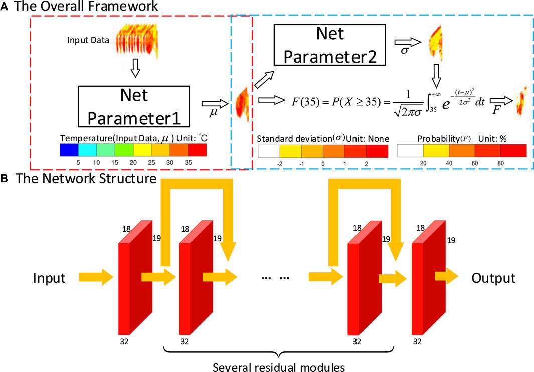
FIGURE 1. (A) Overall framework. The red box is the deterministic forecast module, and the blue box is the probabilistic forecast module. Parameter 1 represents the weights and biases of the trained network in the deterministic forecast, and so does Parameter 2 in the probabilistic forecast. NET is shown in (B). (B) Network structure. The network consists of convolution modules and residual modules.

The network structure is shown in Figure 1B. The size of the input data is 11*18*19(channels*width*height) in the deterministic forecast and 1*18*19 in the probabilistic forecast, which will pass through the single convolution module of the first layer and enter the residual module of the n-layer. Finally, the data will be output through the single convolution module in the size of 1*18*19. Our data will always keep the dimension of 32*18*19, without any other complex transformations during the whole process.

We further introduce the model in this article. The model consists of a convolution module and a residual module. The first layer of convolution transforms the input data into 32 channels of data to facilitate the subsequent calculation of the residual structure. The residual part consists of several residual modules, each consisting of a convolution module and a jump connection with constant mapping (He et al., 2016a; He et al., 2016b). Suppose the input of the ith layer is x, with the convolutional structure (Conv) and the jump connection layer, we obtain Conv(x) and x. Then, they are added together and the output y of the ith residual module is obtained after the activation function (AF). For details, see Equation 1. The use of multiple layers of residuals can always retain the data features of the previous layer, while continuously digging deeper into the data relationships so that the network can memorize previous information in the process of extracting information, and has better training performance compared to the convolutional network, as detailed in Section 4.2.

$y=AF\left(Conv\left(x\right)+x\right).(1)$

2.3 Index and Experimental Setting

Our experiment is divided into the deterministic forecast and probabilistic forecast, corresponding to different evaluation indexes, respectively. We use the mean absolute error (MAE) (Ji et al., 2019), root mean square error (RMSE) (Gneiting et al., 2005), equitable threat score (ETS) (Hamill and Juras, 2006), and anomaly correlation coefficient (ACC) (Ji et al., 2019) as the evaluation index of the deterministic forecast and use brier score (BS) (Weigel et al., 2008), brier skill scores (BSS) (Hamill and Juras, 2006), and continuous ranked probability score (CRPS) (Rasp and Lerch, 2018) as the evaluation index of the probabilistic forecast. They are, respectively, evaluated from the temperature value, fall area, the correlation degree, the probabilistic value, and forecast skill of the probabilistic forecast.

We use a server containing four blocks of Tesla V100 to experiment, and the language platform is Python3.8.5 and Torch 1.6.0. In the deterministic forecast, MAE is the loss function, and in probabilistic forecasting, CRPS is the loss function (Möller and Groß, 2016; Díaz et al., 2020). The optimizer for both experiments is Adam (Kingma and Ba, 2014). We set the learning rate as 0.0001 and perform 500 epochs of study. To achieve stable and effective learning results, we set the super parameters through many experiments and experiences.

In the next section, we compare the multilayer perceptron approach (MLP) and our deep learning approach (Resnet) with the forecast baseline (ECMWF).

3 Experiments

3.1 Deterministic Forecast

In deterministic forecasts, we use models consisting of 1–40 residual network modules to conduct experiments and obtain the respective evaluation results. The next step is to select the optimal model, and it is not easy to guarantee that all the indexes in each model are optimal. To address this situation, we further propose an equal weight voting screening mechanism with the following rules for the same loss function for the same forecast date:

1) The model with four or three dominant indexes is the optimal model.

2) The model with two dominant indexes in the first 15 days is the dominant model, and the model with two dominant indexes other than the ETS index in the last 15 days is the optimal model.

3) The two models each have two dominant indexes, and the model with the loss function corresponding to the dominant index is the optimal model.

4) Each of the four models occupies a dominant indicator, and the model in which the indicator corresponding to the loss function is located is the optimal model.

Finally, we select the 30 best models under each of the two loss functions, as shown in Table 3.

TABLE 3

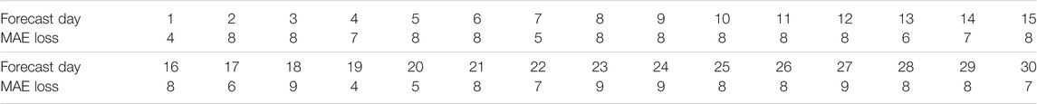
TABLE 3. Number of optimal modules of the model.

In Figure 2, it can be seen that the MLP only outperforms the forecast baseline in the early stage, while our deep learning approach can outperform the forecast baseline across the board. Overall, from the perspective of the whole test set, the deep learning method shows a more comprehensive performance in terms of forecast error, forecast fallout, and correlation coefficient and effectively revises the European hindcast data.

FIGURE 2

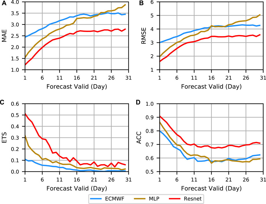
FIGURE 2. Evaluation curves of deterministic forecasts. (A–D) are MAE, RMSE, ETS, and ACC for deterministic forecast assessment, respectively. Different methods are indicated by different colors.

For more visual analysis of the revision effect, the spatial distribution of the mean absolute errors for different forecast durations (1st, 8th, 15th, 22nd, and 29th) is given in Figure 3. In the continental region, the lighter color, such as white and yellow, indicates the smaller difference with the observed value and better effect. Conversely, the darker color, such as orange and red, means that the difference is greater, and the effect is worse. For the baseline, the light-colored areas (errors of 0°C–2°C) are only concentrated in the North China Plain, the middle and lower reaches of the Yangtze River Plain, and the Northeast China Plain on the first day, while in the rest of the regions and forecast days, it is basically covered by darker colors (errors of 2°C–6°C), and even the areas with larger errors, such as near Wushan, show deep red color (errors of more than 6°C). In general, some plain areas have good forecasts, while high mountains, hills, and inland areas have high forecast errors due to their unique geographical factors, such as altitude or unpredictable atmospheric circulation, which makes it difficult for the traditional numerical model to capture the effects of various factors flexibly. In the second column, the revised results of the MLP have improved in the Pearl River and Yangtze River basins, and the overall color is lighter than that of the ECMWF, but in other regions, such as the northern part of the North China Plain and the northeastern corner of Inner Mongolia, negative optimization is produced. It may be since the method only explores the variation pattern of independent grids themselves and lacks attention to the surrounding area. The last column is the lightest in color from the overall view, and the errors do not exceed 5°C in all regions and forecast days which show more regions with errors of 0°C–2°C compared to the results in the first two columns. In difficult spots of baseline, such as the Wushan region and the northern part of the MLP negative optimization, our method can perform effective positive optimization. This shows that the deep learning method based on the residual network provides a more significant effect on the error correction of European hindcast data.

FIGURE 3

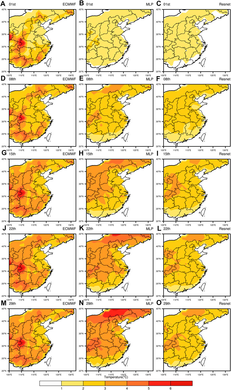
FIGURE 3. Spatial error distribution map for deterministic forecasts. The five rows represent the five forecast days (1st, 8th, 15th, 22nd, and 29th). The three columns are ECMWF (A, D, G, J, and M), MLP (B, E, H, K, and N), Resnet (C, F, I, L, and O).

3.2 Probabilistic Forecast

Probabilistic forecasting is a probabilistic estimate of whether the temperature will be within a certain temperature range based on a deterministic forecast. The 95th percentile of observations covered in this article is approximately 35°C, so we use 35°C as the high temperature threshold for probabilistic forecasting Wulff and Domeisen (2019). The data generated from the training and test sets of the deterministic forecasts after the network revise are used as the training and test sets of the revised probabilistic forecasts, respectively. The probabilistic forecasts of ECMWF are derived through the ensemble members, so there is no CRPS index.

According to BS (A), BSS (B), and CRPS(C) in Figure 4, MLP is superior to ECMWF, which shows that MLP does have some effect in probabilistic forecasting. However, because MLP ignores the relationship between lattice points, there is a large gap between MLP and our deep learning method. In summary, our deep learning method has the optimal effect in probabilistic forecasting.

FIGURE 4

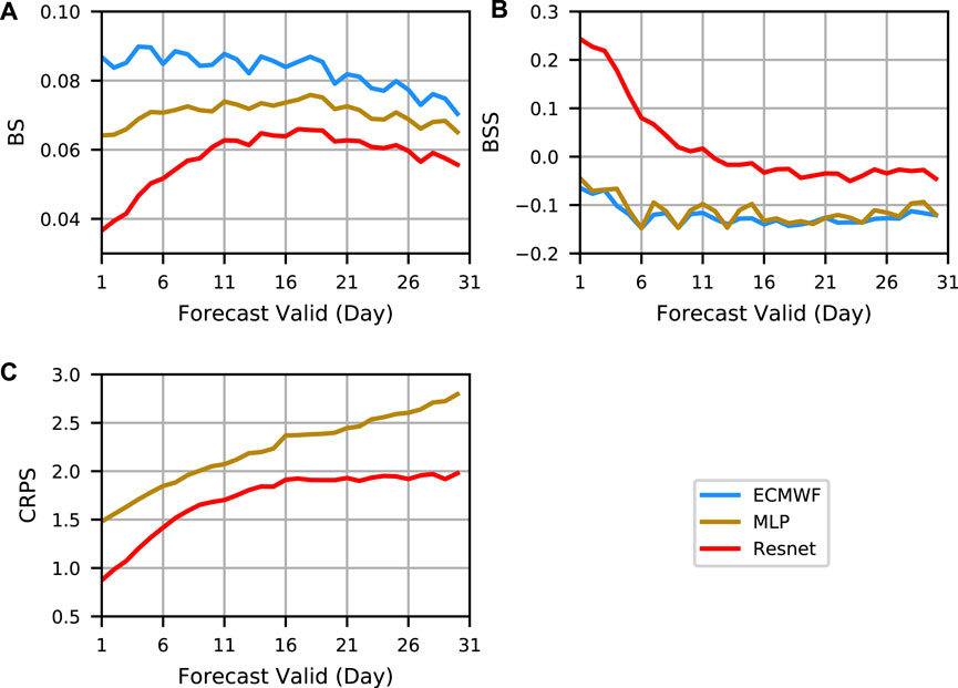
FIGURE 4. Evaluation curves of probabilistic forecasts. (A–C) are BS, BSS, and CRPS for probabilistic forecast assessment, respectively. Different methods are indicated by different colors.

In Figure 5, the probabilistic forecast distribution under five forecast days is shown. It can be seen that ECMWF and MLP can forecast part of the high temperature region in the first forecast day. Resnet, however, is better in the first forecast day: the fallout area and the probability values are larger. The poor results of ECMWF and MLP in the other four forecast days indicate that the probabilistic forecasts of both methods are not meaningful for longer extension periods. In contrast, Resnet successfully forecasts part of the high temperature region for the 8th and 15th forecast days with larger values, which indicates that our method has meaningful forecasts for the extended period.

FIGURE 5

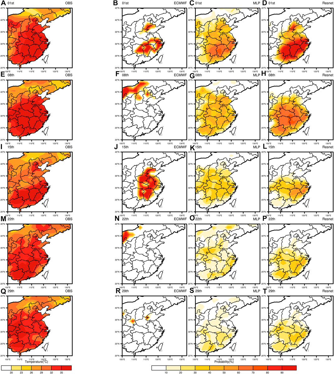
FIGURE 5. Spatial distribution of probabilistic forecasts. The five rows represent the five forecast days (1st, 8th, 15th, 22nd, and 29th). The four columns are Observation (A, E, I, M, and Q), ECMWF (B, F, J, N, and R), MLP (C, G, K, O, and S), and Resnet (D, H, L, P, and T).

4 Discussion

4.1 Reliability Study of Full Version Data

In the experiments, we directly select the training set consisting of four versions for training. From the original re-forecast data, the data of each version only have the overlapping date, and the forecast values are different, whose forecast accuracy will improve as the versions are updated and iterated. So, this then raises the question of whether different versions of data can be trained together. To answer it, we conduct a new experiment comparing four learning methods: same-version learning, cross-version learning, transfer learning, and full-version learning. The same version learning is learning on the training set of the 2017 version and testing on the testing set of the 2017 version. Cross version learning is learning on the training set of the 2016 version and then testing on the testing set of the 2017 version. Transfer learning is learning on the training set of the 2016 version, then learning in small batches on the training set of the 2017 version, and lastly testing on the testing set of the 2017 version.

As shown in Figure 6, all four methods obtain good results, among which the full version of the method shows optimal results in all cases except for slightly worse performance in the late stages of the ETS index. The performance of all methods in order from disadvantage to advantage is cross-version learning, transfer learning, same version learning, and full version learning.

FIGURE 6

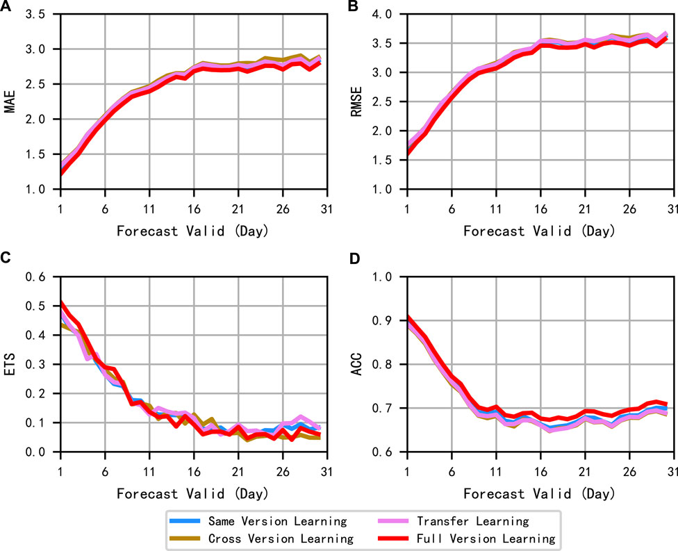
FIGURE 6. Evaluation curves for diverse learning methods. (A–D) are MAE, RMSE, ETS, and ACC, respectively.

Cross-version learning learns in different versions and achieves good results in the target version testing set, which indicates that there is not much difference between versions or even some correlations. Transfer learning is based on cross-version learning in small batches and can obtain slightly better experimental results than cross-versions, which indicates that learning from different versions to learning in small batches on the target version learns as many features as possible while reasonably grasping the feature that there is a correlation between versions and improving the testing results on the target version. The same version learning is only the learning of the target version, which directly finds the data features of the target version, extracting the own features of the target version better than the cross-version learning, and learns the target version more directly than the migration learning. The full-version learning approach mixing all versions of data takes advantage of the existence of certain differences and correlations between different versions to reasonably expand the dataset which leads that the generalization ability and feature learning ability of the model are improved again to finally achieve the best optimal testing results. Thus, different versions of the data can be trained together, and better results can be obtained.

4.2 Ablation Experiment of Residual Module

To verify whether the presence of the residual structure is necessary, we remove the skip branch of the residual module from the previously screened optimal models keeping only the main path convolutional structure.

Figure 7 shows the comparison of the curves of the convolutional model and the residual model under deterministic and probabilistic forecasts, respectively. The effect of the residual network is significantly better than that of the convolutional network, which indicates that the jumping branches of the network play a significant role in the improvement of the overall network performance, and the residual network has better forecasting performance compared with the convolutional network.

FIGURE 7

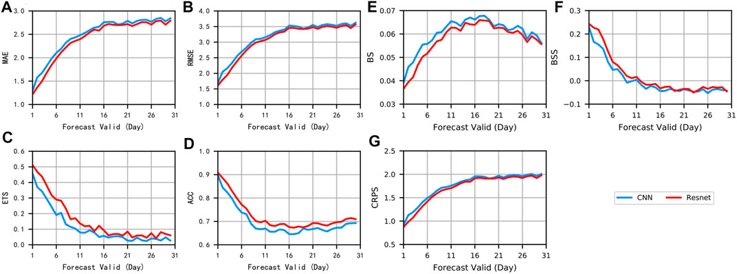
FIGURE 7. Evaluation curves of CNN and Resnet. (A–D) are MAE, RMSE, ETS, and ACC for deterministic forecast assessment, respectively, (E–G) are BS, BSS, and CRPS for probabilistic forecast assessment. Different methods are indicated by different colors.

The indexes are only a presentation of the overall effect and cannot be analyzed from the model itself. Therefore, it is discussed from the view of training point and model parameters. The first forecast day is taken for example: the residual model is four residual blocks, and the corresponding convolution model is four convolution blocks.

The first is the training perspective. Figure 8A shows the loss curve of the first forecast day. The red curve has a lower starting error value while also decreasing and converging faster which is always smaller than the error value of the blue curve inscribed at the same time during the training. This indicates that the residual model trains better and is more suitable for the current research work than the convolutional model. The second is the model parameter angle. Choosing any forecast result in the first forecast day, the observation for that day is shown in Figure 8B.

FIGURE 8

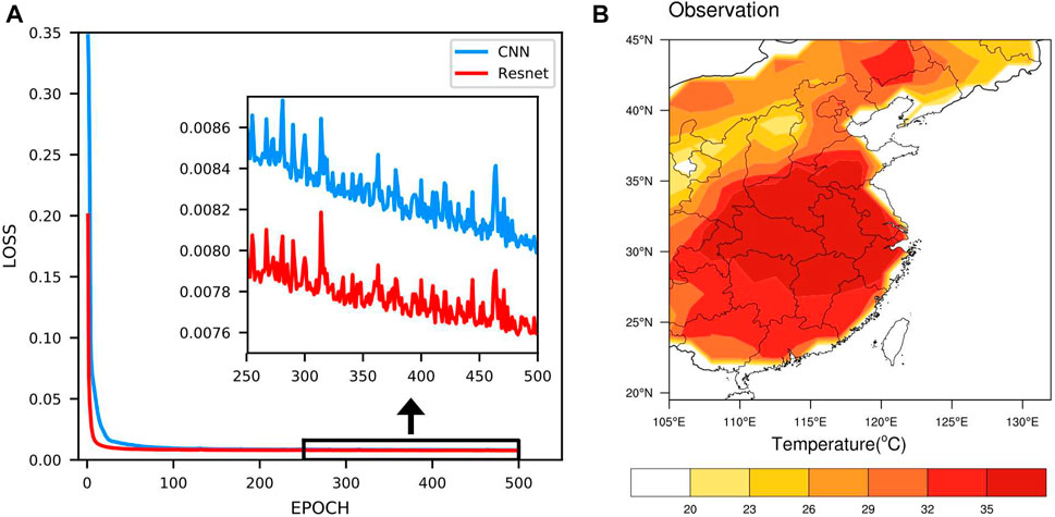
FIGURE 8. (A) Loss plot of CNN and Resnet on the first forecast day. Different methods are indicated by different colors. (B) Observation for the corresponding date.

In the deterministic forecasting, as shown in Figure 9, the parameters of the convolutional model after training are always kept below 0.5, and the variation between the parameters of each layer and different regions is small, which indicates that the model is always trained in a shallow layer only to explore limited superficial connections, and the parameters are adjusted in a relatively stable training way to obtain limited revisions. Such a training approach tends to ignore the deeper data relationships and cannot escape from the local optimum of the model. The parameters of the trained residual model increase from 0 to 0.9 layer by layer, and there is a significant difference between the southeast coastal region and the inland region. This great variation in parameters pushes the model to break the local shackles of stable training and keep searching for a larger range of optimal parameters in each layer of training to obtain a better revision effect. In the error distribution plot on the right, we can see that the red areas with larger errors in the residual model are lighter, meaning that the residual model has a better revised effect on the forecast errors.

FIGURE 9

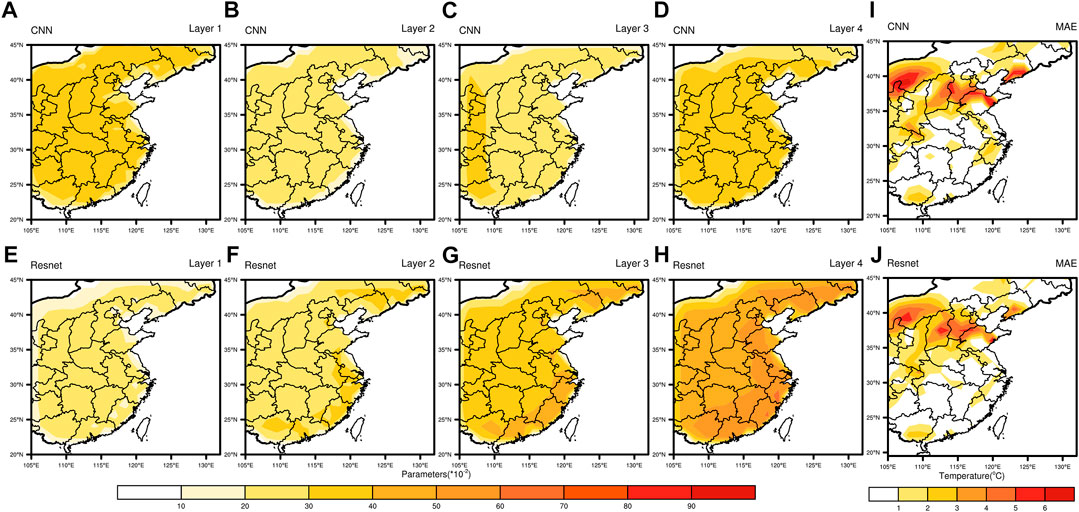
FIGURE 9. Heat map of network parameters and spatial absolute error distribution. It shows changes of average parameters (A–H) of the four modules and the absolute errors (I, J) in the deterministic forecasts. (A–J) are related to the CNN (Resnet).

In the probabilistic forecasting, as shown in Figure 10, the parameters of the convolutional model drop from 10 to less than 1.5 after training, and the color variety of the parameter visualization decreases layer by layer, which demonstrates that the model has captured a considerable amount of feature information from the beginning, but the surface feature extraction is always performed around the output of the previous layer in the subsequent layers of the module. At this point, the extraction capacity of the model is close to saturation, and the model performance has reached the upper limit. The pattern of parameter variation after training of the residual model is just the opposite of the convolutional model, where the parameter visualization progresses from shallow to deep, with each layer revealing new features at a deeper level, resulting in more significant parameter variation. The most intuitive manifestation of this change is in the probabilistic forecasts in the last column, where the residual model forecasts a larger range of high probability high temperature regions concerning the observed values (Figure 8B).

FIGURE 10

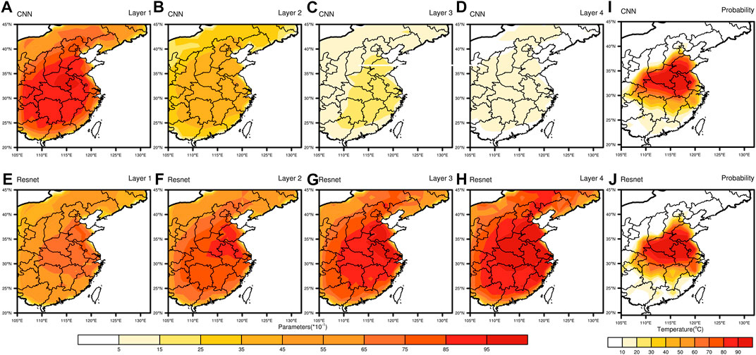
FIGURE 10. Heat map of network parameters and probabilistic distribution. It shows changes of average parameters (A–H) of the four modules and the probabilistic forecasts (I, J) in the probabilistic forecasts. (A–J) are related to the CNN (Resnet).

The superiority of the residual model over the convolutional model is reflected by the almost complete lead of the seven indexes in Figure 7. Overall, the residual module is more advantageous than the convolutional module, and the presence of the residual structure is necessary for this study.

4.3 Analysis of the Effectiveness of Sub-seasonal Forecasting

To analyze the sub-seasonal forecast effects, especially the 35°C forecast effect, this section selects July 29, 2010, as the sample with the most remarkable high temperature among the observations in the testing set (the largest number of 35°C grids on this day, accounting for nearly 50% of the total number of grids in the study area). Then, four sets of data are used in the testing set with an extended period of 30 days and initial dates of July 7, 2010; July 14, 2010; July 21, 2010; and July 28, 2010, in which the sample date corresponds to the 23rd forecast day, the 16th forecast day, the 9th forecast day, and the 2nd forecast day, respectively.

As shown in Figure 11, Resnet is closer to the observed values in the deterministic forecast, indicating that the correction of ECMWF by our method is effective. Compared with the 2nd and 9th forecast days, the effect of the left grid point forecast is significantly lower with longer lead time, which may be due to the spatial distribution of the grid points.

FIGURE 11

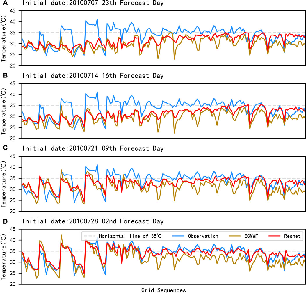
FIGURE 11. Curves of the deterministic forecast by grids on 29 July 2010 under different initial dates. (A–D) are the four different initial dates: 7 July 2010, 14 July 2010, 21 July 2010, and 28 July 2010. The horizontal coordinates are the 174 grids which form a one-dimensional sequence in the order of west to east and north to south in the study area.

As shown in Figure 12, in the probabilistic forecasts, the probability values of some grid points of ECMWF in the second and ninth forecast days are over 50%, indicating that it has some probabilistic forecast value. And in these two forecast days, Resnet can forecast more high temperature areas with higher probability values, showing better probabilistic forecast results than ECMWF. In the 16th and 23rd forecast days, it is difficult for ECMWF to forecast high temperature fallout areas effectively. In contrast, Resnet still forecasts some of the high-temperature fallout areas, which means that our method has some forecasting effectiveness under long extension periods. In addition, we found that Resnet consistently makes incorrect probabilistic forecasts for the rightmost grids, possibly due to the model’s insufficient learning of the probabilistic forecast features for this part.

FIGURE 12

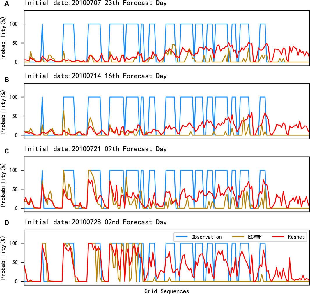
FIGURE 12. Curves of the probabilistic forecast by grids on 29 July 2010 under different initial dates. (A–D) are the four different initial dates: 7 July 2010, 14 July 2010, 21 July 2010, and 28 July 2010. The horizontal coordinates are the 174 grids which form a one-dimensional sequence in the order of west to east and north to south in the study area.

In summary, Resnet has superior forecasting capability compared to ECMWF, which is effective for improving the forecast value of the extended period in probabilistic forecasts while reducing the deterministic forecast error. For some of the grids with poor results, we speculate that there are different sub-seasonal feature spaces in the whole study area, so we will model different areas separately in the future in a more targeted manner.

5 Conclusion

Efficient sub-seasonal forecasting models will provide early warnings of extreme hazards, such as droughts, for the purpose of reducing losses. In this article, the residual structure is first applied with the S2S dataset to generate sub-seasonal forecast. From the selection of dataset to the model, the optimal Resnet model was obtained after a lot of experiments, and finally, a complete sub-seasonal forecasting system was established from deterministic forecasting to probabilistic forecasting. Compared with the forecast benchmark of the ECMWF, MLP, and CNN, the Resnet model achieved excellent forecasting results owing to the fact that it can consider the relationship between grids and has better feature extraction ability. In deterministic forecasting, it is effective in most correcting areas and overcoming the problem of large errors in the Wushan area. In probabilistic forecasting, the probability distribution is predicted by establishing the association between deterministic and probabilistic forecasts, where the forecast positive skill was successfully extended to about 2 weeks and made research more meaningful for extended period forecasting. Our experimental approach can provide a reference for future applications of deep learning in the field of sub-seasonal high temperature forecasting. In the future, more effective methods will be found, such as combining circulation data and trying more advanced models, to improve sub-seasonal high temperature forecasting.

Data Availability Statement

The raw data supporting the conclusions of this article will be made available by the authors, without undue reservation.

Author Contributions

WJ conducted the experiment and edited the manuscript. The other authors contributed the analysis and writing.

Funding

This study was supported by the National Key R&D Program Special Fund Grant (No. 2018YFC1505805), the National Natural Science Foundation of China (Nos. 62072106 and 61070062), the General Project of Natural Science Foundation in Fujian Province (No. 2020J01168), and the Open project of Fujian Key Laboratory of Severe Weather (No. 2020KFKT04).

Conflict of Interest

The authors declare that the research was conducted in the absence of any commercial or financial relationships that could be construed as a potential conflict of interest.

Publisher’s Note

All claims expressed in this article are solely those of the authors and do not necessarily represent those of their affiliated organizations, or those of the publisher, the editors, and the reviewers. Any product that may be evaluated in this article, or claim that may be made by its manufacturer, is not guaranteed or endorsed by the publisher.

References

Brunet, G., Shapiro, M., Hoskins, B., Moncrieff, M., Dole, R., Kiladis, G. N., et al. (2010). Collaboration of the Weather and Climate Communities to advance Subseasonal-To-Seasonal Prediction. Bull. Amer. Meteorol. Soc. 91, 1397–1406. doi:10.1175/2010BAMS3013.1

CrossRef Full Text | Google Scholar

Cohen, J., Coumou, D., Hwang, J., Mackey, L., Orenstein, P., Totz, S., et al. (2019). S2s Reboot: An Argument for Greater Inclusion of Machine Learning in Subseasonal to Seasonal Forecasts. Wires Clim. Change 10, e00567. doi:10.1002/wcc.567

CrossRef Full Text | Google Scholar

Díaz, M., Nicolis, O., Marín, J. C., and Baran, S. (2020). Statistical post‐processing of ensemble forecasts of temperature in Santiago de Chile. Meteorol. Appl. 27, e1818. doi:10.1002/met.1818

CrossRef Full Text | Google Scholar

Durai, V. R., and Bhradwaj, R. (2014). Evaluation of Statistical Bias Correction Methods for Numerical Weather Prediction Model Forecasts of Maximum and Minimum Temperatures. Nat. Hazards 73, 1229–1254. doi:10.1007/s11069-014-1136-1

CrossRef Full Text | Google Scholar

Gel, Y. R. (2007). Comparative Analysis of the Local Observation-Based (Lob) Method and the Nonparametric Regression-Based Method for Gridded Bias Correction in Mesoscale Weather Forecasting. Weather Forecast. 22, 1243–1256. doi:10.1175/2007WAF2006046.1

CrossRef Full Text | Google Scholar

Gneiting, T., Raftery, A. E., Westveld, A. H., and Goldman, T. (2005). Calibrated Probabilistic Forecasting Using Ensemble Model Output Statistics and Minimum Crps Estimation. Monthly Weather Rev. 133, 1098–1118. doi:10.1175/MWR2904.1

CrossRef Full Text | Google Scholar

Guan, H., Zhu, Y., Sinsky, E., Li, W., Zhou, X., Hou, D., et al. (2019). Systematic Error Analysis and Calibration of 2-m Temperature for the Ncep Gefs Reforecast of the Subseasonal experiment (Subx) Project. Weather Forecast. 34, 361–376. doi:10.1175/WAF-D-18-0100.1

CrossRef Full Text | Google Scholar

Hamill, T. M., and Juras, J. (2006). Measuring Forecast Skill: Is it Real Skill or Is it the Varying Climatology? Q.J.R. Meteorol. Soc. 132, 2905–2923. doi:10.1256/qj.06.25

CrossRef Full Text | Google Scholar

He, K., Zhang, X., Ren, S., and Sun, J. (2016a). “Deep Residual Learning for Image Recognition,” in Proceedings of the IEEE Conference on Computer Vision and Pattern Recognition (CVPR). doi:10.1109/cvpr.2016.90

CrossRef Full Text | Google Scholar

He, K., Zhang, X., Ren, S., and Sun, J. (2016b). “Identity Mappings in Deep Residual Networks,” in European Conference on Computer Vision (Springer), 630–645. doi:10.1007/978-3-319-46493-0_38

CrossRef Full Text | Google Scholar

He, S., Li, X., DelSole, T., Ravikumar, P., and Banerjee, A. (2020). Sub-seasonal Climate Forecasting via Machine Learning: Challenges, Analysis, and Advances. arXiv preprint arXiv:2006.07972.

Google Scholar

Hwang, J., Orenstein, P., Cohen, J., Pfeiffer, K., and Mackey, L. (2019). “Improving Subseasonal Forecasting in the Western U.S. With Machine Learning,” in Proceedings of the 25th ACM SIGKDD International Conference on Knowledge Discovery & Data Mining, 2325–2335. doi:10.1145/3292500.3330674

CrossRef Full Text | Google Scholar

Ji, L., Zhi, X., Zhu, S., and Fraedrich, K. (2019). Probabilistic Precipitation Forecasting over East Asia Using Bayesian Model Averaging. Weather Forecast. 34, 377–392. doi:10.1175/WAF-D-18-0093.1

CrossRef Full Text | Google Scholar

Kingma, D. P., and Ba, J. (2014). Adam: A Method for Stochastic Optimization. arXiv preprint arXiv:1412.6980.

Google Scholar

Manrique-Suñén, A., Gonzalez-Reviriego, N., Torralba, V., Cortesi, N., and Doblas-Reyes, F. J. (2020). Choices in the Verification of S2s Forecasts and Their Implications for Climate Services. Monthly Weather Rev. 148, 3995–4008. doi:10.1175/MWR-D-20-0067.1

CrossRef Full Text | Google Scholar

Merryfield, W. J., Baehr, J., Batté, L., Becker, E. J., Butler, A. H., Coelho, C. A. S., et al. (2020). Current and Emerging Developments in Subseasonal to Decadal Prediction. Bull. Am. Meteorol. Soc. 101, E869–E896. doi:10.1175/BAMS-D-19-0037.1

CrossRef Full Text | Google Scholar

Möller, A., and Groß, J. (2016). Probabilistic Temperature Forecasting Based on an Ensemble Autoregressive Modification. Q.J.R. Meteorol. Soc. 142, 1385–1394. doi:10.1002/qj.2741

CrossRef Full Text | Google Scholar

Pegion, K., Kirtman, B. P., Becker, E., Collins, D. C., LaJoie, E., Burgman, R., et al. (2019). The Subseasonal experiment (Subx): A Multimodel Subseasonal Prediction experiment. Bull. Am. Meteorol. Soc. 100, 2043–2060. doi:10.1175/BAMS-D-18-0270.1

CrossRef Full Text | Google Scholar

Peng, T., Zhi, X., Ji, Y., Ji, L., and Tian, Y. (2020). Prediction Skill of Extended Range 2-m Maximum Air Temperature Probabilistic Forecasts Using Machine Learning post-processing Methods. Atmosphere 11, 823. doi:10.3390/atmos11080823

CrossRef Full Text | Google Scholar

Phakula, S., Landman, W. A., Engelbrecht, C. J., and Makgoale, T. (2020). Forecast Skill of Minimum and Maximum Temperatures on Subseasonal‐to‐Seasonal Timescales over South Africa. Earth Space Sci. 7, e2019EA000697. doi:10.1029/2019EA000697

CrossRef Full Text | Google Scholar

Rasp, S., and Lerch, S. (2018). Neural Networks for Postprocessing Ensemble Weather Forecasts. Monthly Weather Rev. 146, 3885–3900. doi:10.1175/MWR-D-18-0187.1

CrossRef Full Text | Google Scholar

Son, S. W., Kim, H., Song, K., Kim, S. W., Martineau, P., Hyun, Y. K., et al. (2020). Extratropical Prediction Skill of the Subseasonal‐to‐Seasonal (S2S) Prediction Models. J. Geophys. Res. Atmos. 125, e2019JD031273. doi:10.1029/2019JD031273

CrossRef Full Text | Google Scholar

Vigaud, N., Tippett, M. K., Yuan, J., Robertson, A. W., and Acharya, N. (2019). Probabilistic Skill of Subseasonal Surface Temperature Forecasts over north america. Weather Forecast. 34, 1789–1806. doi:10.1175/WAF-D-19-0117.1

CrossRef Full Text | Google Scholar

Vijverberg, S., Schmeits, M., van der Wiel, K., and Coumou, D. (2020). Subseasonal Statistical Forecasts of Eastern U.S. Hot Temperature Events. Monthly Weather Rev. 148, 4799–4822. doi:10.1175/MWR-D-19-0409.1

CrossRef Full Text | Google Scholar

Weigel, A. P., Baggenstos, D., Liniger, M. A., Vitart, F., and Appenzeller, C. (2008). Probabilistic Verification of Monthly Temperature Forecasts. Monthly Weather Rev. 136, 5162–5182. doi:10.1175/2008MWR2551.1

CrossRef Full Text | Google Scholar

Wulff, C. O., and Domeisen, D. I. V. (2019). Higher Subseasonal Predictability of Extreme Hot European Summer Temperatures as Compared to Average Summers. Geophys. Res. Lett. 46, 11520–11529. doi:10.1029/2019GL084314

CrossRef Full Text | Google Scholar

Xiang, B., Lin, S. J., Zhao, M., Johnson, N. C., Yang, X., and Jiang, X. (2019). Subseasonal Week 3-5 Surface Air Temperature Prediction during Boreal Wintertime in a GFDL Model. Geophys. Res. Lett. 46, 416–425. doi:10.1029/2018GL081314

CrossRef Full Text | Google Scholar

Zhu, Y. (2005). Ensemble Forecast: A New Approach to Uncertainty and Predictability. Adv. Atmos. Sci. 22, 781–788. doi:10.1007/BF02918678

CrossRef Full Text | Google Scholar