A Method for Solving Percolation Overflow Boundary Based on Maximum of Horizontal Energy Loss Rate

Introduction

Seepage is an influencing factor that must be considered in civil engineering, such as the instability of banks and dams caused by seepage (Fox et al., 2006; Chu-Agor et al., 2008; Midgley et al., 2013); the anti-seepage of dams, channels, and buried sites (Mishra and Singh, 2005; Charles et al., 2010; John and Michael Duncan, 2010; Xu et al., 2013); and the problems related to seepage encountered in specific engineering (Kobayashi and de los Santos, 2007; Lu and Chiew, 2007; Hung et al., 2009; Batool and Brandon, 2013). The solution to these problems depends on the calculation of the seepage field. Therefore, finding a reasonable way to calculate the seepage field has always been an important research topic (Healy and Laak, 1974; Bhagu, 2007; Lai and Liang, 2008; Kazumasa and Kaneda., 2010; Chen, 2017; Li, 2017; Peng, 2017). The finite element method is widely used in the calculation of seepage fields because it can be applied to complex boundaries and complex soil layers. In past studies, the virtual element method (Wu and Zhang, 1994; Cui and Zhu, 2009), element penetration matrix adjustment method (Huang et al., 2001; Zhu and Liu, 2001), initial flow method (Pan et al., 1998; Wang, 1998), and some other finite element calculation methods of seepage field (Wang et al., 2003; Zhang, 2004; Xie and Zhang, 2005) are reasonable calculation methods of seepage field under known boundary conditions. However, the overflow boundary of the seepage field is usually unknown, so it is impossible to define the boundary before finite element calculation. For the determination of overflow boundary, scholars have proposed some solutions. Wu and Zhang (1994) proposed that within the possible overflow boundary, a row of lower points is assumed to be overflow points. The nodes below the overflow point are known nodes, and the nodes above are unknown nodes. The water head of each node of the seepage field is calculated and the free surface is iterated until it converges. The water head of the upper point of the overflow point is compared with its elevation. If the water head is less than the elevation, the assumed overflow point position is reasonable. Otherwise, the upper point shall be taken as the overflow point and recalculated until the requirements are met. Zhu and Liu (2001) pointed out that the overflow boundary can be regarded as the second type of boundary condition. After calculating the flow, it can be transformed into the first type of boundary condition by adjusting the free term. When dealing with the overflow boundary, Huang et al. (2001) define the points on the overflow boundary as fixed points and active points according to the relationship between the water head and elevation and finally finds the location of the overflow point through iteration and linear interpolation. In the equivalent permeability coefficient method, Xie and Zhang (2005) iterated the overflow point with the free surface according to the difference between the water head and elevation until the absolute value of the difference between the water head and elevation is less than the convergence value. There are two problems in the above method: firstly, the overflow point and the free surface need to be iterated together in the calculation of the overflow boundary, and the initial overflow point assignment is based on empirical estimation, so there will be a problem of non-convergence; secondly, the basis for determining the overflow boundary is usually only when the local element or node meets a certain condition, and it is not analyzed from the perspective of the whole seepage field.

Li et al. (2016) proposed a method to solve the overflow boundary based on the principle of minimum global total potential energy. By analyzing the water head distribution trend of the seepage field under different overflow boundary conditions, this method identified the boundary that minimizes the global total potential energy as the real overflow boundary. Hou and Sun (2019) put forward the concept of total potential energy in the real area on this basis, eliminated the influence of seepage virtual area, and considered that the overflow boundary that minimizes the total potential energy in seepage real area is the real overflow boundary. The above two methods make up for the problems existing in the previous overflow point, which do not need an iterative calculation and determination method from the perspective of the energy of the whole calculation area. However, the total potential energy is a scalar index, and the directionality of the hydraulic gradient in the boundary conditions of the overflow point cannot be considered. Therefore, the method of considering the total potential energy is not sufficient. If we can investigate the directional index, it is an improvement to this kind of method.

To sum up, based on the principle of global total potential energy minimization, through the analysis of the water head distribution of seepage field under different overflow boundaries, this paper puts forward a method to solve the overflow boundary based on the maximum of horizontal energy loss rate. It is considered that the overflow boundary that makes the horizontal energy loss rate of the seepage field reach the maximum is the real overflow boundary. This method not only retains the advantages of the original method but also considers the directionality of water flow and makes the physical meaning more clear.

The Application of Variational Principle in Finite Element Calculation of Seepage Field

In the two-dimensional seepage field, a rectangular coordinate system is established with the bottom of the upstream slope as the origin of coordinates, the horizontal direction from upstream to downstream as the positive axis direction, and the vertically upward direction as the positive axis direction. According to Darcy’s law and seepage continuity conditions, regardless of the compressibility of soil and water, the steady seepage of homogeneous anisotropic soil satisfies the following partial differential equations:

$k_x\frac{{\partial }^{2}h}{\partial x^2}+k_z\frac{{\partial }^{2}h}{\partial z^2}=0(1)$

In Eq. 1, k_x and k_z are the permeability coefficients in x and z directions, and h is the water head function.

According to the variational principle, the solution of the above differential equation can be transformed into finding the extreme value of the function, and a function shown in Eq. 2 can be constructed:

$I\left(h\right)={\displaystyle \underset{\text{Ω}}{\iint }\frac{1}{2}\left[k_x{\left(\frac{\partial h}{\partial x}\right)}^2+k_z{\left(\frac{\partial h}{\partial z}\right)}^2\right]}dxdz(2)$

Substitute Eq. 2 into Euler’s equation and its boundary condition, it can be obtained that:

$\frac{\partial }{\partial x}\left(k_x\frac{\partial h}{\partial x}\right)+\frac{\partial }{\partial z}\left(k_z\frac{\partial h}{\partial z}\right)=0(3)$

${\left(k_x\frac{\partial h}{\partial x}dz-k_z\frac{\partial h}{\partial z}dx\right)}_{\Gamma }=\text{0}(4)$

It is easy to know that Eq. 3 is equivalent to Eq. 1, that is, when h can make the functional Eq. 2 reach an extreme value, this h can satisfy the governing equation of seepage, thus transforming the original differential equation problem into the extreme value problem of function.

Eq. 4 is the boundary condition that naturally forms in the process of variational differentiation, and all unknown boundaries will be given such boundary conditions. Let n be the outer normal vector of the boundary Γ, then dx/dΓ = cos (n,z) = l_z, dz/dΓ = −cos (n,x) = −l_x, so after dividing Eq. 4 by dΓ, we can get:

$k_x\frac{\partial h}{\partial x}{l}_x+k_z\frac{\partial h}{\partial z}{l}_z=k_n\frac{\partial h}{\partial n}=0(5)$

Eq. 5 indicates that the flow across the boundary is zero. That is, when applying the variational principle to solve the seepage field, if the boundary is not assigned, the unknown boundary will be given impervious boundary conditions.

Solving Overflow Boundary Based on the Maximum Horizontal Energy Loss Rate

The Physical Significance of Solving Seepage Field Based on the Variational Principle

The hydraulic gradient in the x and z directions at any point in the seepage field is $i_x=\partial h/\partial x$ and $i_z=\partial h/\partial z$. According to the formula of permeability, $j_x={\gamma }_w{i}_x={\gamma }_w\partial h/\partial x$ and $j_z={\gamma }_w{i}_z={\gamma }_w\partial h/\partial z$ are the components of osmotic force in x and z directions, respectively (γ_w is the unit weight of water); according to Darcy’s law, $v_x=k_x\partial h/\partial x$ and $v_z=k_z\partial h/\partial z$ are the seepage velocity in x and z directions, respectively. Analyze the integrand function in Eq. 2:

$k_x{\left(\frac{\partial h}{\partial x}\right)}^2+k_z{\left(\frac{\partial h}{\partial z}\right)}^2=k_x{i}_x{i}_x+k_z{i}_z{i}_z=\left(v_x{j}_x+v_z{j}_z\right)/{\gamma }_w(6)$

The part in parentheses on the right side of the Eq. 6 is a manifestation of power, and its physical meaning is the work done by water to unit soil in unit time. By integrating Eq. 6, the work done by water to the soil per unit time in the whole seepage area can be obtained, so the function defined in Eq. 2 is proportional to the energy loss rate in the whole seepage area. According to the principle of minimum work, when the variation of function is zero by the water head function, the energy loss rate of the whole seepage area reaches the minimum, that is, the obtained head function does not depend on the instantaneous balance of a certain physical quantity but represents the distribution of the water head in a stable state where the energy loss rate reaches the minimum.

Water Head Distribution Under Different Overflow Boundaries

Suppose the real seepage field is shown in Figure 1A-1, BC and DE are the upstream and downstream boundaries; BF is the free surface boundary, which divides the seepage field into two parts: upper h < z and lower h > z; F is the overflow point and EF is the real overflow boundary; AB, AG, GF, and CD are all impermeable boundaries. Taking the seepage field under the real overflow boundary as the initial state, the horizontal hydraulic gradient that makes the water head decrease in the positive direction along the x-axis is defined as positive. When part of the real overflow boundary is suddenly defined as an impervious boundary (FF_L in Figure 1A-2), the horizontal rightward hydraulic gradient that is originally existing at FF_L is defined as zero, which reduces the total value of the hydraulic gradient in the horizontal direction of the whole seepage field. When the seepage field reaches stability according to the principle of minimum energy disappearance rate, the horizontal rightward hydraulic gradient of the seepage field will be smaller than that in the initial state. When part of the original impermeable boundary is suddenly defined as the overflow boundary (as FF_H in Figure 1A-3), the part originally satisfying h < z is defined as h = z, so that there is a horizontal leftward hydraulic gradient in this area, and when the seepage field reaches stability according to the principle of minimum energy disappearance rate, the horizontal hydraulic gradient of seepage field will also be smaller than the initial state. Therefore, the horizontal hydraulic gradient of the seepage field will reach its maximum value under the real overflow boundary.

FIGURE 1

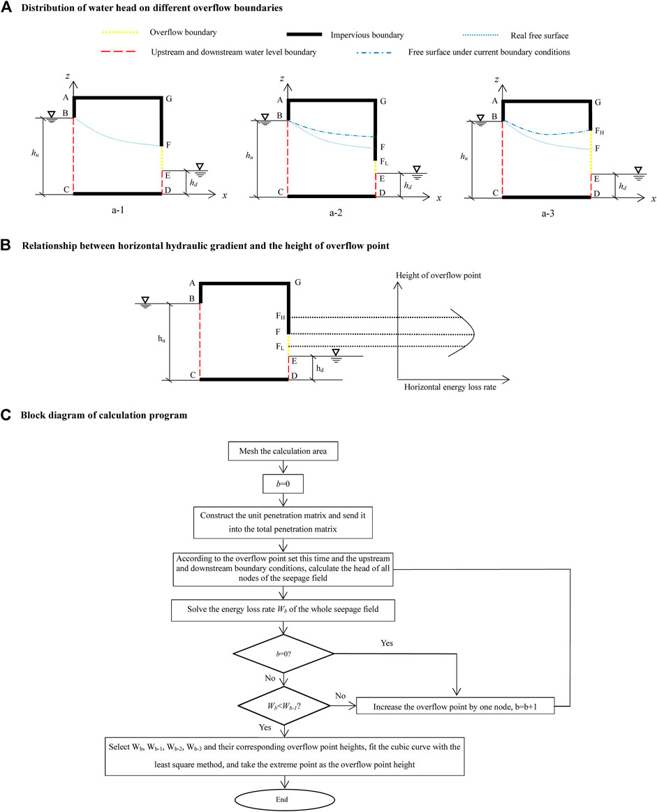
FIGURE 1. Model information. (A) Distribution of the water head on different overflow boundaries. (B) The relationship between horizontal hydraulic gradient and the height of overflow point. (C) A block diagram of calculation program.

Selection of Calculation Indexes and Calculation Steps

In previous studies, two methods, global and real domain total potential energy, were used to calculate the overflow point. However, the total potential energy selected by this method is a scalar index, and the water flow on the overflow boundary has the directionality pointing out of the domain. Therefore, it is not completely accurate to control the overflow boundary only with the total potential energy (when adjusting the overflow point, the vertical hydraulic gradient will also affect the total potential energy and the position of the extreme point). Therefore, the directional index should be selected to control the overflow point calculation. Since the physical significance of horizontal hydraulic slope is not clear, the horizontal energy loss rate proportional to the square of the horizontal hydraulic slope is selected as the calculation index. Dividing the global domain into finite elements, and the horizontal energy loss rate W_e in any element is as follows:

$W_e={\displaystyle \underset{e}{\iiint }{\gamma }_w{k}_x{\left(\frac{\partial h}{\partial x}\right)}^{2}dxdz}(7)$

The horizontal energy loss rate in the whole seepage field is as follows:

$W={\displaystyle \sum W_e}(8)$

It is worth noting that when the horizontal energy loss rate is selected as the consideration index, due to the existence of the square term, the hydraulic gradient that is originally negative (horizontally leftward) will also increase the horizontal energy loss rate and cause errors. Therefore, for elements with a negative total hydraulic gradient, the horizontal energy loss rate should be defined as negative. Combined with the above theoretical analysis, when the overflow point is the true value, the horizontal energy loss rate of the seepage field will reach a minimum value (as shown in Figure 1B).

Specific Fortran program calculation steps are as follows:

Step (1): Compile data files according to element division, including the total number of elements, element node number information, coordinate information of main nodes, number of soil types, element number occupied by each type of soil, the permeability coefficient of each type of soil, upstream and downstream water level values, number of upstream and downstream water level nodes, number of nodes that may overflow boundaries, and node numbers that may overflow boundaries.

Step (2): Read all the information in the data file.

Step (3): Make b = 0. Construct the element permeability matrix based on the element information and feed it into the overall permeability matrix according to the node number of the seepage field.

Step (4): Adjust the overall infiltration matrix and free terms according to the upstream and downstream boundary conditions, and the existing overflow point (the highest node downstream is used as the overflow point when b = 0). Calculate the linear equation system to obtain the nodal water head of the seepage field.

Step (5): Determine whether b is greater than 0. If yes, perform step 6; if no, perform step (7).

Step (6): Based on the element node-water head and element information, solve the horizontal energy loss rate of each element and record the horizontal energy loss rate W_b of the seepage area with water flowing through it. Compare W_b-1 and W_b, if W_b > W_b-1, execute step (7); if W_b < W_b-1, execute step (8).

Step (7): Raise the overflow point by one node, b = b + 1, and return to step (4).

Step (8): Select W_b, W_b-1, W_b-2, W_b-3, and their corresponding overflow point heights; apply the least square method to fit the cubic curve; and take the extreme value point where W_b is closer to the corresponding overflow point height value as the overflow point height (when b < 3, take the overflow node corresponding to W_b-1 as the overflow point height).

The block diagram of the calculation procedure is shown in Figure 1C.

Numerical Examples

To verify the correctness of this method, two models with experimental solutions are calculated.

A Model With a Glycerol Experimental Solution

For the rectangular earth dam with a 6-m upstream water level, 1-m downstream water level, and impervious bottom, the glycerolysis at the overflow point is 3.25 m (Mao et al., 1999). It is divided by isosceles right-angle six-node triangular element with a right-angle side length of 1 m, and the finite element model with 48 elements and 117 nodes is obtained. Under different overflow points, the horizontal energy loss rate is shown in Table 1. After fitting the cubic curve with the least square method, the extreme value is 3.304. The difference with the experimental solution of glycerol is 0.054 m, and the relative error is only 1.64%. To verify the impact of element division on the accuracy of the method, it is divided by isosceles right-angle six-node triangular element with a right-angle side length of 0.2 m, and the finite element model with 1,200 elements and 2,501 nodes is obtained. Under different overflow points, the horizontal energy loss rate is shown in Table 1. After fitting the cubic curve with the least square method, the extreme value is 3.292 m. The difference with the experimental solution of glycerol is 0.042 m, and the relative error is only 1.28%. The calculation accuracy is improved.

TABLE 1

TABLE 1. Horizontal energy loss rate with different number of elements.

A Model With an Experimental Solution of Electrical Simulation

The size of the three-dimensional electric simulation model is 10 m $\times$ 10 m $\times$ 1 m; the permeability coefficient k is the same in x, y, and z directions; and the water level at the upstream and downstream of soil is 10 and 2 m, respectively. Its bottom is an impervious boundary, and the electrical simulation solution of the seepage overflow point is 4.74 m. Divided into hexahedron elements with a side length of 0.5 m, there are 800 elements and 1,323 nodes. The 3D calculation model and the calculation results are listed in Figure 2.

FIGURE 2

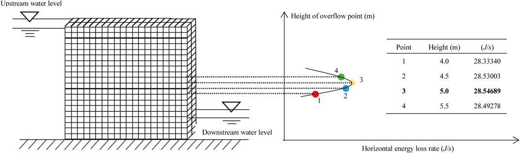
FIGURE 2. Three-dimensional (3D) model division and calculation results of energy loss rate.

The cubic curve fit to the node vertical coordinates and the corresponding energy loss rate is performed by the least square method, and the resulting cubic curve equation with a cubic term coefficient of −0.15763, a quadratic term coefficient of −2.49713, a primary term coefficient of 13.07164, and a constant term of 5.91232 is calculated as the extreme value point of 4.787 m. The difference with the actual overflow point location was 0.047 m and 0.98%. The comparison with other methods is shown in Table 2.

TABLE 2

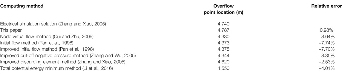
TABLE 2. Accuracy comparison of overflow points with published results.

Conclusion

Based on the analysis of functional physics meaning in variational principle and the characteristics of the water head distribution under different overflow boundary conditions, this paper puts forward a method to solve overflow boundary based on the maximum value of horizontal energy loss rate, expounds the theoretical basis, calculates the three-dimensional electrical simulation experimental model, and obtains the following conclusions:

According to the physical meaning of function and the characteristics of the water head distribution under different overflow boundary conditions, this paper considers that the overflow boundary with the maximum energy loss rate is the real overflow boundary. When determining the overflow boundary, it is not necessary to iterate the overflow point and the free surface together, so the calculation is simple, and there is no problem of non-convergence. Selecting horizontal energy loss rate as a comparison index is more explicit than the physical meaning of total potential energy. By calculating the model with glycerol experimental solution under different mesh densities, the relative error of overflow point is only 1.64% and 1.28%. The finer the mesh is, the smaller the relative error is, which verifies the rationality of the method. Compared with the results of overflow points calculated by the three-dimensional electrical simulation solution model, the relative error of overflow points calculated by this method is only 0.98%. Compared with the overflow points calculated by node virtual flow method, initial flow method, improved initial flow method, improved cut-off negative pressure method, and improved discharging element method, this method has a small relative error and superiority accuracy. It can be used as a method to determine seepage overflow points.

Data Availability Statement

The original contributions presented in the study are included in the article/Supplementary Material. Further inquiries can be directed to the corresponding author.

Author Contributions

XL and ZZ conceptualized the study. YL, BH, and LJ performed mathematical derivation. YL and LJ made significant contributions in the computer program. QD validated and curated the data. YL and LJ were responsible for writing: original draft preparation, review, and editing. All authors contributed to the article and approved the submitted version.

Funding

This study is supported by the National Natural Science Foundation of China (Grants: 51808290, U2039208, and U1839202, which are gratefully acknowledged).

Conflict of Interest

The authors declare that the research was conducted in the absence of any commercial or financial relationships that could be construed as a potential conflict of interest.

Publisher’s Note

All claims expressed in this article are solely those of the authors and do not necessarily represent those of their affiliated organizations or those of the publisher, the editors, and the reviewers. Any product that may be evaluated in this article, or claim that may be made by its manufacturer, is not guaranteed or endorsed by the publisher.

References

Batool, A., and Brandon, T. L. (2013). Analytical Calibration Approach to Develop a Seepage Model for the London Avenue Canal Load Test. J. Geotech. Geoenviron. Eng. 139 (5), 788–796. doi:10.1061/(asce)gt.1943-5606.0000810

CrossRef Full Text | Google Scholar

Bhagu, R. C. (2007). Analysis of Seepage from Polygon Channels. J. Hydraulic Eng. 133 (4), 451–460. doi:10.1061/(ASCE)0733-9429

CrossRef Full Text | Google Scholar

Charles, M., Sierra Orvis, B., and Alexander, N. (2010). Canal Seepage Reduction by Soil Compaction. J. Irrigation Drainage Eng. 136 (7), 479–485. doi:10.1061/(ASCE)IR.1943-4774.0000205

CrossRef Full Text | Google Scholar

Chen, J. (2017). Experimental Study of Stress and Permeability Property of Compacted Bentonite with Cracks under Water Intrusion. Rock Soil Mech. 2, 487–492. doi:10.16285/j.rsm.2017.02.023

CrossRef Full Text | Google Scholar

Chu-Agor, M. L., Wilson, G. V., and Fox, G. A. (2008). Numerical Modeling of Bank Instability by Seepage Erosion Undercutting of Layered Streambanks. J. Hydrol. Eng. 13 (12), 1133–1145. doi:10.1061/(asce)1084-0699(2008)13:12(1133)

CrossRef Full Text | Google Scholar

Cui, H., and Zhu, Y. (2009). Improved Procedure of Nodal Virtual Flux of Global Iteration to Solve Seepage Free Surface. J. Wuhan Univ. Tech. (Transportation Sci. Engineering) 33 (2), 238–241. doi:10.3963/j.issn.1006-2823.2009.02.010

CrossRef Full Text | Google Scholar

Fox, G. A., Wilson, G. V., Periketi, R. K., and Cullum, R. F. (2006). Sediment Transport Model for Seepage Erosion of Streambank Sediment. J. Hydrol. Eng. 11 (6), 603–611. doi:10.1061/(asce)1084-0699(2006)11:6(603)

CrossRef Full Text | Google Scholar

Healy, K. A., and Laak, R. (1974). Site Evaluation and Design of Seepage Fields. J. Envir. Engrg. Div. 100 (5), 1133–1146. doi:10.1061/jeegav.0000254

CrossRef Full Text | Google Scholar

Hou, X., and Sun, W. (2019). Calculation Method of Seepage Overflow Point Based on the Real Domain Total Potential Energy. J. Geotechnical Engineer 2019, 6034526. doi:10.1155/2019/6034526

CrossRef Full Text | Google Scholar

Huang, W., Liu, Y., and Zhou, C. (2001). Finite Element Algorithm for 3-D Unconfined Seepage Flow Field. J. Hydraulic Eng. 8, 49–52. doi:10.3321/j.issn:0559-9350.2001.06.007

CrossRef Full Text | Google Scholar

Hung, M.-H., Lauchle, G. C., and Wang, M. C. (2009). Seepage-Induced Acoustic Emission in Granular Soils. J. Geotech. Geoenviron. Eng. 135 (4), 566–572. doi:10.1061/(asce)1090-0241(2009)135:4(566)

CrossRef Full Text | Google Scholar

John, D., and Michael Duncan, R. J. (2010). Findings of Case Histories on the Long-Term Performance of Seepage Barriers in Dams. J. Geotechnical Geoenvironmental Eng. 136 (1), 2–15. doi:10.1061/(ASCE)GT.1943-5606.0000175

CrossRef Full Text | Google Scholar

Kazumasa, M., and Kaneda., T. (2010). Boundary Condition of Groundwater Flow through Sloping Seepage Face. J. Hydrologic Eng. 15 (9), 718–724. doi:10.1061/(ASCE)HE.1943-5584.0000233

CrossRef Full Text | Google Scholar

Kobayashi, N., and de los Santos, F. J. (2007). Irregular Wave Seepage and Overtopping of Permeable Slopes. J. Waterway, Port, Coastal, Ocean Eng. 133 (4), 245–254. doi:10.1061/(asce)0733-950x(2007)133:4(245)

CrossRef Full Text | Google Scholar

Lai, D., and Liang, R. (2008). Coupled Creep and Seepage Model for Hybrid Media. J. Eng. Mech. 134 (3), 217–223. doi:10.1061/(asce)0733-9399(2008)134:3(217)

CrossRef Full Text | Google Scholar

Li, L. (2017). Development of Testing System for Coupled Seepage and Triaxial Stress Measurements and its Application to Permeability Characteristic Test on Filling Medium. Rock Soil Mech. 10, 3053–3061. doi:10.16285/j.rsm.2017.10.035

CrossRef Full Text | Google Scholar

Li, Y., Hou, X., Zheng, S., and Sun, W. (2016). Calculation Method of Seepage Overflow Point Based on the Principle of Minimum Total Potential Energy. J. Water Resour. Architectural Eng. 14 (4), 84–88. doi:10.3969/j.issn.1672-1144.2016.04.017

CrossRef Full Text | Google Scholar

Lu, Y., and Chiew, Y.-M. (2007). Seepage Effects on Dune Dimensions. J. Hydraul. Eng. 133 (5), 560–563. doi:10.1061/(asce)0733-9429(2007)133:5(560)

CrossRef Full Text | Google Scholar

Mao, C., Duan, X., and Li, Z. (1999). Numerical Computation in Seepage Flow and Programs Application. Nanjing: Hohai University Press.

Google Scholar

Midgley, T. L., Fox, G. A., Wilson, G. V., Heeren, D. M., Langendoen, E. J., and Simon, A. (2013). Seepage-Induced Streambank Erosion and Instability: In Situ Constant-Head Experiments. J. Hydrol. Eng. 18 (10), 1200–1210. doi:10.1061/(asce)he.1943-5584.0000685

CrossRef Full Text | Google Scholar

Mishra, G. C., and Singh, A. K. (2005). Seepage through a Levee. Int. J. Geomech. 5 (1), 74–79. doi:10.1061/(asce)1532-3641(2005)5:1(74)

CrossRef Full Text | Google Scholar

Pan, S., Wang, Q., and Yu, J. (1998). Analysis of Improvement of Free Surface Percolation Using Initial Flow Method. J. Geotechnical Engineer 83, 68–73. doi:10.3321/j.issn:1000-4548(2012)02-0202-08

CrossRef Full Text | Google Scholar

Peng, S. (2017). Experimental Study on Shear-Seepage of Coupled Properties for Complete sandstone under the Action of Seepage Water Pressure. Rock Soil Mech. 10, 3053–3061. doi:10.16285/j.rsm.2017.08.008

CrossRef Full Text | Google Scholar

Wang, J., Wu, Y., and Bai, C. (2003). Flow Element Method with Free Surface Analysis. Hydroelectric Energ. Sci. 21 (4), 23–26. doi:10.3963/j.issn.1000-7709(2003)04-0023-03

CrossRef Full Text | Google Scholar

Wang, Y. (1998). The Modified Initial Flow Method for 3-D Unconfined Seepage Computation. J. Hydraulic Eng. 83, 68–73. doi:10.1088/1755-1315/69/1/012170

CrossRef Full Text | Google Scholar

Wu, M., and Zhang, X. (1994). Imaginary Element Method for Numerical Analysis of Seepage with Free Surface. J. Hydraulic Eng. 8, 67–71. doi:10.3969/j.issn.0559-9350.1994.01.022

CrossRef Full Text | Google Scholar

Xie, G., and Zhang, G. (2005). An Improved Method of Two-Dimensional Pressureless Steady Flow Analysis. Earth Environ. 51, 52–56. doi:10.3969/j.issn.1672-9250.2005.z1.011

CrossRef Full Text | Google Scholar

Xu, Q., Powell, J., Tolaymat, T., and Townsend, T. G. (2013). Seepage Control Strategies at Bioreactor Landfills. J. Hazard. Tox. Radioact. Waste 17 (4), 342–350. doi:10.1061/(asce)hz.2153-5515.0000185

CrossRef Full Text | Google Scholar

Zhang, Q., and Wu, Z. (2005). The Improved Cut-Off Negative Pressure Method for Unsteady Seepage Flow with Free Surface. Chin. J. Geotechnical Eng. 27 (1), 48–54. doi:10.3321/j.issn:1000-4548.2005.01.007

CrossRef Full Text | Google Scholar

Zhang, W., and Xiao, M. (2005). Study on Optimizing Abandoning Element Method for Numerical Analysis of Seepage with Free Surface and its Application in Underground Engineering. J. Water Resour. Architectural Eng. 3 (1), 32–36. doi:10.3969/j.issn.1672-1144.2005.01.009

CrossRef Full Text | Google Scholar

Zhang, Y. (2004). Using the Equivalent Permeability Coefficient to Search the Surface of Seepage. J. Eng. Geology. 02, 177–192.

Google Scholar

Zhu, J., and Liu, G. (2001). An Improved Method for Calculating Unconfined Seepage with Changing Element Conductivity Matrix. J. Hydraulic Eng. 8, 49–52. doi:10.3321/j.issn:0559-9350.2001.08.009

CrossRef Full Text | Google Scholar