 Erica Spain1,2*
 Geoffroy Lamarche3
 Vanessa Lucieer1
 Sally J. Watson2
 Yoann Ladroit2,4
 Erin Heffron5
 Arne Pallentin2
 Joanne M. Whittaker1
- 1Institute for Marine and Antarctic Studies, University of Tasmania, Hobart, TAS, Australia
- 2National Institute of Water and Atmospheric Research, Wellington, New Zealand
- 3School of Environment, University of Auckland, Auckland, New Zealand
- 4ENSTA Bretagne, Brest, France
- 5Center for Coastal and Ocean Mapping, Joint Hydrographic Center, University of New Hampshire, Durham, NH, United States
Understanding fluid expulsion is key to estimating gas exchange volumes between the seafloor, ocean, and atmosphere; for locating key ecosystems; and geohazard modelling. Locating active seafloor fluid expulsion typically requires acoustic backscatter data. Areas of very-high seafloor backscatter, or “hardgrounds,” are often used as first-pass indicators of potential fluid expulsion. However, varying and inconsistent spatial relationships between active fluid expulsion and hardgrounds means a direct link remains unclear. Here, we investigate the links between water-column acoustic flares to seafloor backscatter and bathymetric metrics generated from two calibrated multibeam echosounders. Our site, the Calypso hydrothermal vent field (HVF) in the Bay of Plenty, Aotearoa/New Zealand, has an extensive catalogue of vents and seeps in <250 m water depth. We demonstrate a method to quantitatively link active fluid expulsion (flares) with seafloor characteristics. This allows us to develop predictive spatial models of active fluid expulsion. We explore whether data from a low (30 kHz), high (200 kHz), or combined frequency model increases predictive accuracy of expulsion locations. This research investigates the role of hardgrounds or surrounding sediment cover on the accuracy of predictive models. Our models link active fluid expulsion to specific seafloor characteristics. A combined model using both the 30 and 200 kHz mosaics produced the best results (predictive accuracy: 0.75; Kappa: 0.65). This model performed better than the same model using individual frequency mosaics as input. Model results reveal active fluid expulsion is not typically associated with the extensive, embedded hardgrounds of the Calypso HVF, with minimal fluid expulsion. Unconsolidated sediment around the perimeter of and between hardgrounds were more active fluid expulsion sites. Fluids exploit permeable pathways up to the seafloor, modifying and refashioning the seafloor. Once a conduit self-seals, fluid will migrate to a more permeable pathway, thus reducing a one-to-one link between activity and hardgrounds. Being able to remotely predict active and inactive regions of fluid expulsion will prove a useful tool in rapidly identifying seeps in legacy datasets, as well as textural metrics that will aid in locating nascent, senescent, or extinct seeps when a survey is underway.
Introduction
Seafloor fluid expulsion is a key mechanism for large-scale gas exchange between the seafloor, ocean (Mcginnis et al., 2006; Reeburgh, 2007), and potentially the atmosphere (Gentz et al., 2014; Sahling et al., 2014; Shakhova et al., 2014; Römer et al., 2017). Anomalous areas of very-high seafloor acoustic backscatter, or “hardgrounds,” are often used as first-pass indicators of fluid expulsion sites, in addition to water-column acoustic anomalies, or “flares.” Hardgrounds form via several seafloor fluid expulsion processes: persistent mineral precipitation of oxides, sulfides, and minerals from hydrothermal fluids (Stoffers et al., 1999; Canet, 2003; Prol-Ledesma et al., 2004; Noé et al., 2006); hydrothermal alteration of the seafloor (Hocking et al., 2010; Monecke et al., 2014); or microbial mediation, whereby archaeal microbes oxidize dissolved gasses in escaping bubbles, forming authigenic carbonate platforms (Levin, 2005; Judd and Hovland, 2009; Finkl and Makowski, 2016). Anomalous very-high seafloor backscatter areas have higher backscatter intensities than the surrounding seafloor are thus interpreted as ‘hardgrounds,’ as lithified seafloor is a stronger scatterer than the surrounding soft sediment. The relationship between acoustic hardgrounds and observable areas of indurated, lithified seafloor indicative of these processes has been validated in numerous settings (Judd and Hovland, 2009; Conti et al., 2016; Mitchell et al., 2018; Thorsnes et al., 2019; Phrampus et al., 2020; Watson et al., 2020).
A direct link between active fluid expulsion and acoustic hardgrounds however remains unclear. Varying and inconsistent spatial relationships between observable fluid expulsion, hardgrounds, and the surrounding seafloor have been noted previously (Naudts et al., 2008; Naudts et al., 2010; Thorsnes et al., 2019). This unclear relationship reflects the complexity of hardground genesis, gas migration, fluid expulsion processes, and spatio-temporal differences in expulsion and embedment. Active fluid expulsion can be both short- (decades) or long-lived (thousands of years) (Judd and Hovland, 2009; Levin et al., 2016). Fluids exploit permeable pathways upward to the seafloor, with preliminary seafloor expression (either liquid or gas bubble expulsion) often occurring in areas of soft unconsolidated sediment due to an unrestricted pathway (Levin, 2005; Judd and Hovland, 2009). Hardground formation begins within the subsurface and, given enough time, can become embedded on the seafloor. Once the conduit closes or ceases activity, hardgrounds will remain at the surface or in the subsurface, with surface hardgrounds thenceforth observable in seafloor acoustic backscatter (Judd and Hovland, 2009; Levin et al., 2016). Formalizing the link between gas flares and hardgrounds has thus remained elusive due to spatiotemporal differences between active expulsion and hardground formation, which can post-date expulsion activity.
Here, we present a study from the active Calypso hydrothermal vent field (HVF), in the offshore Taupō Volcanic Zone, Aotearoa/New Zealand to address whether there are measurable links between gas flares, as a proxy for active fluid expulsion, and seafloor characteristics, in particular hardgrounds. Calypso HVF represents a rich laboratory of active fluid expulsion, in gas and liquid form, with a mix of vents, seeps, and hardground features, with a formal catalogue of active fluid expulsion spanning over five decades (Duncan and Pantin, 1969; Glasby, 1971; Sarano et al., 1989; Stoffers et al., 1999; Botz et al., 2002; Mitchell et al., 2004; Lamarche and Barnes, 2005; Schwarz-Schampera et al., 2007; Hocking et al., 2010; Wysoczanski et al., 2015).
Our dataset encompasses bathymetry and backscatter from two calibrated multibeam echosounders (MBES) operating simultaneously at 200 and 30 kHz (nominal) frequencies. Seafloor backscatter reflectivity and penetration depends, in part, on the signal frequency or aperture of the chosen MBES, as well as the acoustic impedance characteristics of the seafloor (a function of the medium’s density and consequent sound speed) (Jackson et al., 1986; Guillon and Lurton, 2001; Huff, 2008). The acoustic response, or backscatter intensity returned, is dependent on interactions between wavelength, seafloor roughness, seafloor scattering regime (a function of substrate particle size), and volume scattering effects (a function of signal penetration), once radiometric and geometric compensations are applied (Urick, 1956; Medwin and Clay, 1997; Hughes Clarke, 2015). The seafloor backscatter mosaic produced may therefore not directly correlate to the feature of interest if the MBES penetration potential is too high or low. Specific to hardgrounds, the MBES frequency may be unable to reveal hardgrounds embedded beneath the surface unless it can penetrate to the appropriate depths or may not accurately capture surface expressions if the frequency is too low.
Here, we use a classification approach, involving image segmentation and random forest modelling, to:
1 Quantitatively link water-column acoustic flares (here considered as a proxy for active fluid expulsion) with specific seafloor characteristics to determine potential links to hardgrounds in this region;
2 Assess whether these specific seafloor characteristics can be used to develop predictive spatial models of active fluid expulsion;
3 Evaluate if a low (nominally 30 kHz), high (200 kHz), or a combined frequency model increases predictive accuracy of seafloor fluid expulsion; and
4 Investigate the role hardgrounds or surrounding sediment cover may have on the accuracy of a predictive model.
Materials and Methods
The Calypso Hydrothermal Vent Field
The Calypso HVF is a well-known gas-hydrothermal region of the offshore Taupō Volcanic Zone (TVZ), in the center of the Bay of Plenty, Aotearoa/New Zealand. It lies ∼40 km offshore Te Ika-a-Māui/North Island and 7 km SW of the Whakaari/White Island active volcano (Figure 1A) (Sarano et al., 1989; Stoffers et al., 1999; Botz et al., 2002). The Calypso HVF is part of the Central Volcanic Region, that represents the volcanically active back-arc region of the Hikurangi subduction system located ca. 300 km to the east. The extensional tectonic setting associated with the back-arc has resulted in a dense network of NE-SW trending normal faults (Wright, 1992), expressed at the seafloor by a pervasive system of scarps (Lamarche and Barnes, 2005). The TVZ extends offshore from the Bay of Plenty coast into the NE-trending depression of the Whakatāne Graben.
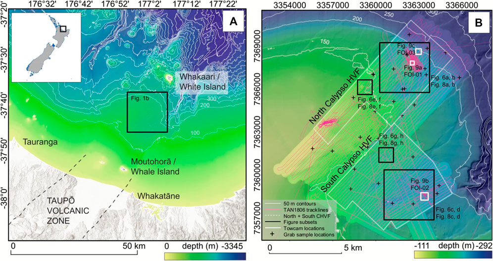
FIGURE 1. (A) Bay of Plenty, Aotearoa/New Zealand (inset map) bathymetry, the offshore Taupō Volcanic Zone (TVZ). The Calypso HVF (black box) sits between Whakaari/White Island and Moutohorā/Whale Island (black dashed lines: TVZ approximate boundaries; white lines: 100 m contours;). (B) Calypso HVF 5 m bathymetry, collected during TAN1806, draped over regional bathymetry (white lines: 50 m contours; pink lines: vessel track; white dashed boxes: clipped North and South Calypso HVF regions; white boxes: towed camera locations; black crosses: sediment grab locations).
Active fluid expulsion was formally catalogued at Calypso HVF from water-column acoustic scattering and visible sea surface bubbles (Duncan and Pantin, 1969; Glasby, 1971) and then from video observations (Sarano et al., 1989; Hocking et al., 2010). These fluid expressions are evidence of both diffuse and discrete gas emission, predominantly CH4 and CO2, from submarine geothermal activity (Stoffers et al., 1999; Botz et al., 2002). Calypso HVF fluid expulsion is suggested to be structurally controlled by the pervasive NE-SW trending fault system, with observed fluid expulsion ephemerality inferred to be related to seismic activity (Pantin and Wright, 1994). Stoffers et al. (1999) observed numerous active fluid expulsion areas aligned with fault scarps. In addition to the North Calypso HVF (including the original Calypso site from Sarano et al. (1989)) a second site, now known as the South Calypso HVF, was also detected with two discrete zones of fluid expulsion (Stoffers et al., 1999). Subsequent voyages produced bathymetric maps of the area (25 m grid resolution) using a Kongsberg EM302 (30 kHz) MBES and generated a good knowledge of the tectonic fabric along with surface, water-column, and seafloor evidence for fluid expulsion and mineral precipitation (Mitchell et al., 2004; Schwarz-Schampera et al., 2007; Wysoczanski et al., 2015).
Multibeam Data Acquisition and Processing
Data were acquired during the 2018 RV Tangaroa voyage TAN 1806, a component of the international project QUOI: “Quantitative Ocean-column Imaging using hydroacoustic sources” (Lamarche et al., 2019). The TAN1806 survey employed Kongsberg EM 2040 (200 kHz) and EM302 (30 kHz) MBES to map the Calypso HVF, operated synchronously. Both MBES systems are hull-mounted on RV Tangaroa. MBES compensation occurred at the start of the voyage at the NIWA test-patch sites in Palliser Bay and Palliser Bank, Aotearoa/New Zealand. Calibration was undertaken over multiple depths on seafloor zones with flat, homogenous sedimentology of silt or sand (Lamarche et al., 2011; Lucieer and Lamarche, 2011; Ladroit et al., 2017). Lines were run for each MBES setting (frequency/pulse) anticipated. Backscatter correction curves were generated to compensate for beam pattern variations by: 1) removing all Kongsberg backscatter corrections, 2) modeling the backscatter angular variations, and 3) modeling the EM302 transducer beam pattern.
Sound velocity profiles (SVP) were taken at 12-h intervals during operations, 3-h intervals during compensation, at the start of new mapping areas, or when noticeable artefacts appeared in the data. MBES data were acquired via Kongsberg Seafloor Information System (SIS) software (v4.2.1) and cleaned in Caris HIPS/SIPS (v10.4). Vessel position, motion, SVP, and tidal corrections were merged with raw range/angle data to generate geolocated soundings. Manual cleaning removed remaining invalid soundings and data spikes. A bathymetric grid at 5 m resolution was produced in NZTM projection (EPSG:2193) (Figure 1B).
Active Fluid Expulsion Identification
Active fluid expulsion was identified in the EM302 MBES (30 kHz) water-column backscatter data using the QPS FM Mid-Water (v7.7.4) Feature Detect tool. Acoustic anomalies detected were analyzed in QPS Fledermaus (v7.7.4) (Figure 2). Acoustic anomalies that were attached to the seafloor, “flares,” were classed as potential fluid expulsion features or “seeps,” indicative of gas bubbles emitting from the seafloor. Point clusters of potential seeps were exported to MATLAB and filtered based on a maximum distance between points (40 m), minimum number of points (200), and aspect ratio (1) of each cluster. A seafloor or “seep base” location was determined for each seep; locations were exported as a point shapefile.
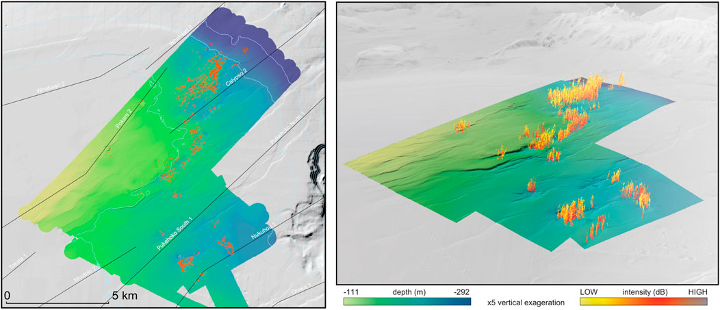
FIGURE 2. Plan and 3D view of water-column acoustic flares collected on the TAN1806 survey overlain Calypso HVF bathymetry (colored) and regional Bay of Plenty bathymetry (greyscale). Plan view show seep base locations (orange points) and fault lines (black lines) from Litchfield et al. (2013).
Bathymetric Derivatives
Bathymetric derivatives were calculated in the ArcGIS spatial analysis toolbox Benthic Terrain Modeler (BTM; v3.0) (Wright et al., 2012; Walbridge et al., 2018). Derivative layers were created using a standard 3 × 3 neighborhood window. All bathymetric derivatives are described in Table 1.
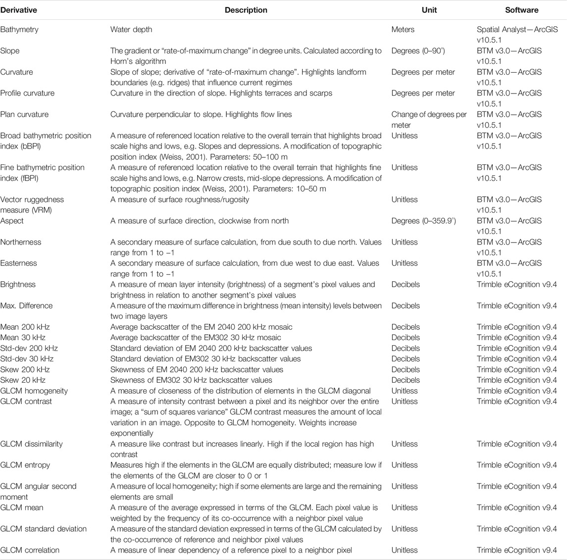
TABLE 1. Bathymetric and backscatter derivatives generated for modelling. All bathymetric derivatives are calculated using a moving 3 × 3 window (Moore’s neighborhood).
Seafloor Backscatter
MBES seafloor backscatter data were imported into SonarScope software (IFREMER, France; Augustin (2016)). Bathymetric sounding validity flags from Caris HIPS/SIPS were applied to corresponding backscatter samples. Kongsberg backscatter corrections applied at time of recording were removed while compensation for local backscatter angular variation and a transmit beam pattern were applied to ensure precise data reduction (Lurton and Lamarche, 2015). Very high overlap of MBES lines during the survey allowed only beams outside nadir (-20°/20°) to be considered, with an average backscatter (decibel, dB) value calculated from multiple samples for each grid point. Backscatter mosaics of both frequencies (200 and 30 kHz) were produced at 2 m resolution (Figure 3).
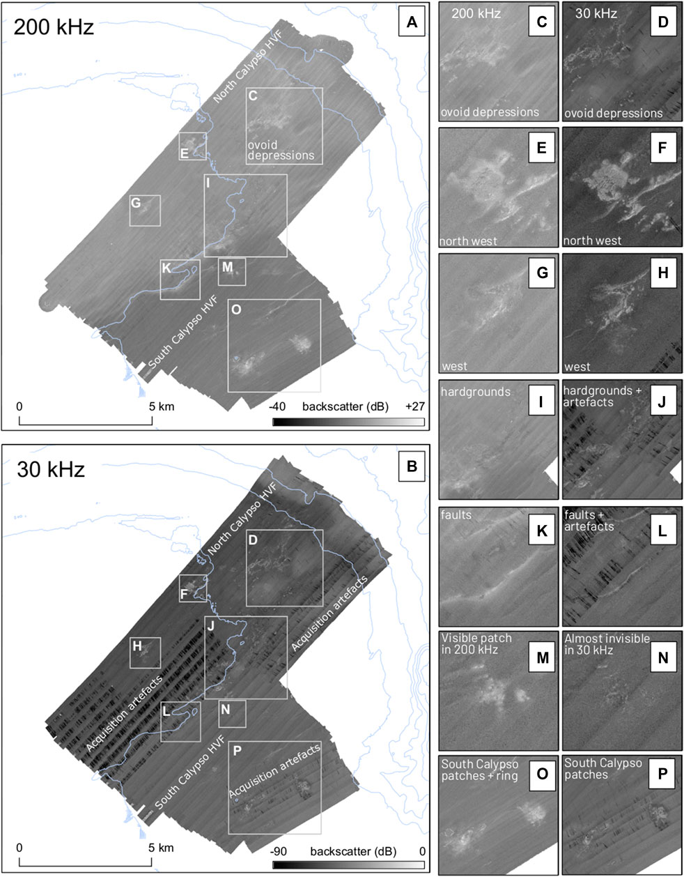
FIGURE 3. Original Calypso HVF EM 2040 (200 kHz) backscatter mosaic (A), and Calypso HVF EM302 (30 kHz) backscatter mosaic (B), (C), (D), (E), (F), (G), (H), (I), (J), (K), (L), (M), (N), (O), (P) insets show detailed comparisons between the two backscatter mosaics. High backscatter intensities (high reflectivity = harder substrate) are lighter; low backscatter intensities (low reflectivity = softer substrates) are darker. Blue lines are 50 m contours; mosaic resolution 2 m; projection NZTM. Very dark areas (black) in the 30 kHz mosaic show acquisition artefacts from aeration of the transducer due to rough sea conditions. Although original mosaic ranges shown include extreme outliers, color ramps are normalized here to ensure comparable grey tones. Mosaic distributions predominantly lie within −30–−5 dB.
An averaging filter (3 × 3 moving window) was passed over the backscatter mosaic to interpolate small pixel-wide gaps from missing data. Both mosaics were clipped from −30 dB to −5 dB to remove large areas of no data and mosaic artefacts (outliers). Both mosaics were classified individually, following Jenks Natural Breaks method (Jenks, 1967) to highlight comparable and dissimilar backscatter classes within each mosaic (Figure 4). Jenks method sorts values into natural classes by reducing the variance within classes while maximizing variance between classes (Jenks, 1967).
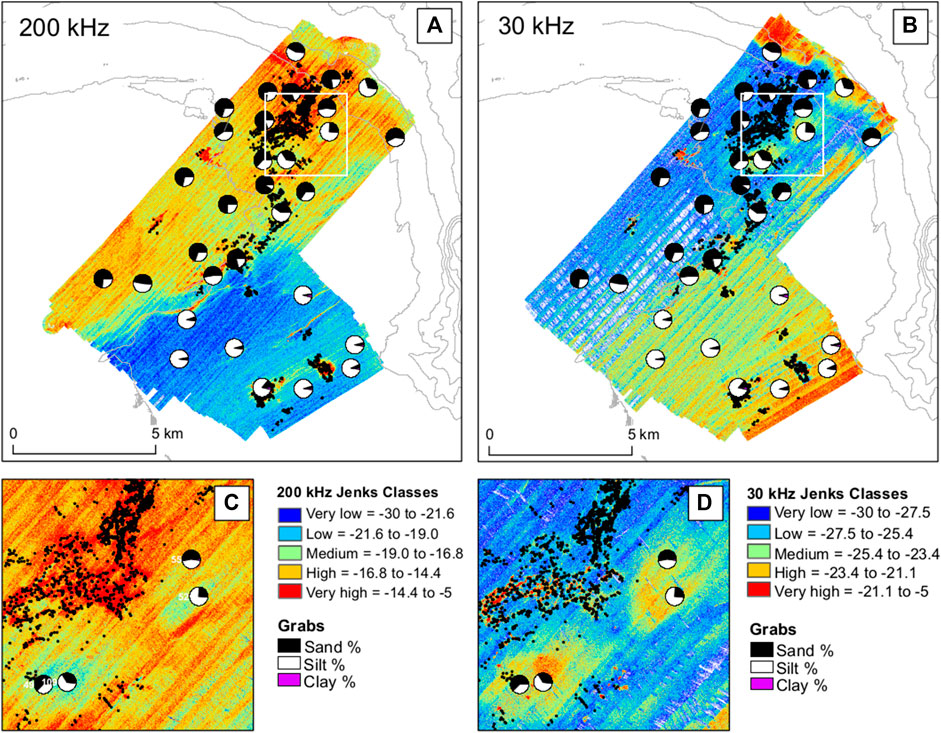
FIGURE 4. Sediment grab results and Jenks Natural Breaks backscatter classes for (A) Calypso HVF 200 kHz mosaic, and (B) Calypso HVF 30 kHz mosaic. Grab results show sand-dominant classes in the North and silt-dominant classes in the South (grey lines: 50 m contours; black dots: seep base locations; mosaic resolution: 2 m; projection: NZTM). Inset of 200 kHz (C) and of 30 kHz (D) show two depressions in North Calypso HVF, with grab samples within each classified as coarse or very coarse silt.
Segmentation of Seafloor Acoustic Data
Backscatter mosaics were segmented using Geographic Object Based Image Analysis (GEOBIA) to identify homogenous regions of seafloor for input into a random forest model. This was achieved using a multiresolution segmentation algorithm in eCognition software (v9.4). Three mosaic configurations were segmented, with bathymetry incorporated in each: 1) 200 kHz backscatter only, 2) 30 kHz backscatter only, and 3) equally weighted EM2040 and EM302 backscatter. Three regions were segmented: the full Calypso HVF dataset, the North Calypso HVF subset, and the South Calypso HVF subset. The individual Calypso HVF regions were analyzed separately to: 1) account for the large differences in acoustic response observed between the north and south (Figure 3); 2) remove the influence of poor weather acquisition artefacts in the North Calypso HVF 30 kHz mosaic (Figure 3B); and 3) account for the historic classification of the Calypso HVF—the North Calypso HVF region includes the data described by Duncan and Pantin (1969), while the South Calypso HVF includes the South flare areas, described by Stoffers et al. (1999) and Botz et al. (2002).
Each mosaic configuration and region were segmented using seven different scale parameters (SPs): 9, 14, 26, 46, 50, 75, and 100. The Estimation of Scale Parameter tool (ESP2) (Dragut et al., 2010) was used to determine the appropriate SP for analysis. The SP is a unitless term to describe the minimum size of the segments. SP levels of 9, 14, 26, and 46 were selected automatically using ESP2. Larger, manually selected SPs (50, 75, and 100) were also interrogated to explore differences between auto- and manually selected SPs. We selected segmentation settings that emphasize the influence of color (greyscale color heterogeneity, in the case of backscatter mosaics) rather than shape (shape = 0.1, color = 0.9). For eCognition, shape and color parameters influence each other (high influence of color equals low influence of shape, and vice versa). Compactness (border length/area) and smoothness of the boundary were equally weighted (0.5) with the aim of extracting backscatter areas with a high color contrast to surrounding seafloor (i.e. “hardgrounds”). Segments along the immediate perimeter of the survey area were removed to avoid edge effects created from backscatter processing.
Similar to the original Jenks classification of individual mosaics (pixel-based classification), segments were classified into five classes based on mean backscatter intensity values (derived from all pixels that contribute to a segment), following Jenks Natural Breaks method (Jenks, 1967) (object-based classification). The five classes reflect the mean backscatter values for each segment from lowest to highest values and each class capturing internally homogenous areas of seafloor (Figure 6).
Textural Analysis of Backscatter Layers
Statistical attributes were generated for each segment, including brightness (combined intensity of both mosaics), maximum difference (backscatter dB difference), and the mean, standard deviation, and skewness of both the 200 and 30 kHz mosaics (Table 1). These values are calculated from all pixel backscatter dB levels that construct each individual image segment. Each segment produces one value for each measure.
Textural values were also generated for each segment in eCognition using the Haralick grey level co-occurrence matrix (GLCM) (Haralick et al., 1973). Texture metrics are commonly used to identify differences between seafloor substrates or associated habitats and can be used as input layers for seafloor classification models (Lucieer, 2008; Buscombe, 2017). Specific to hardground and fluid expulsion in a shallow hydrothermal system, GLCM texture variables provide high-resolution seafloor characteristics in areas where large topographic changes are limited (i.e. flat seafloor). Here, we used the invariant direction, which is the sum of values for four spatial directions (0°, 45°, 90°, and 135°), for the two mosaics individually and then combined. The GLCM analyses relationships between two pixels at a time, a reference and neighbor pixel, using an offset of 1 pixel (i.e. direct neighbor pixels). All backscatter derivative descriptions are provided in Table 1.
Each segmentation layer (for each mosaic configuration and SP) was exported as a shapefile with all textural and geomorphic values attached to each segment. The segment layers and a point shapefile of flare locations (from Section 3.4) were linked in ArcGIS. Segments that were co-located with flare locations were classed as “active” segments and those without flare locations were classed as “inactive.” This process created attribute tables for each segmentation layer with each unique underlying textural and geomorphic values for all ‘active’ and “inactive” segments. Sixty-three joined attribute files were exported as a. csv file for further analysis.
Random Forest Classification
The segment attribute files exported in Section 3.6 were used as input data for random forest (RF) classification. The data encompass seven different SP (9, 14, 26, 46, 50, 75, and 100), three layers from different frequencies (30 kHz mosaic, 200 kHz mosaic, and a combined mosaic (equally weighted) of the two frequencies) and three regions (the full Calypso HVF dataset, the North Calypso HVF subset, and the South Calypso HVF subset).
Supervised RF models were run on each individual exported attribute file, executed in the “randomForest” R package (Liaw and Weiner, 2002). The RF algorithm trains an ensemble of decision trees by randomly selecting and testing a random subset of predictor variables at each node and then pooling all tree results (Brieman, 2001). The RF algorithm was chosen due to its ability to deal with unbalanced classes (as is the case with “active” and “inactive” seafloor segments (Mellor et al., 2015) and its robustness against over-fitting (Lucieer et al., 2012; Buscombe and Grams, 2018). The data sets were randomly split into two groups—training data (70%) for model development and test data (30%) for model evaluation. Binary “presence/absence” (i.e. “active” vs “inactive”) classes were the target. Attribute values from each segment were the predictor variables: backscatter mean, standard deviation, and skewness; backscatter derivatives (GLCM textures), water depth, and bathymetric derivatives (BTM layers). Each model ran with 500 trees and the square root of the number of predictor variables as the subset at each node (rounded down).
Error matrices and model performance statistics (Kappa, sensitivity, specificity, positive predictive value (PPV), and negative predictive value (NPV)) were calculated for each model. Error matrices compare known class data to predicted classes in a 2 × 2 table (true positive, true negative, false positive, and false negative). Model “goodness” thresholds were determined by Kappa values. This value allows for model comparison by quantifying the accuracy of each model above that of chance: 0 = predictive power no better than chance, 0–0.2 = poor, 0.2–0.4 = fair, 0.4–0.6 = moderate, 0.6–0.8 = good and 0.8–1 = very good, 1 = perfect predictive power (Altman, 1991). Sensitivity conveys the ratio of true positive predictions (flare presence) to the total positive observations (i.e. number of correct seep predictions to the number of actual seeps). Specificity conveys to the ratio of true negative predictions (seep absence) to the total negative observations. PPV conveys the ratio of true presence predictions to the total positive predictions (i.e. number of correct seep predictions to the number of positive predictions). NPV denotes the ratio of true negative predictions to the total negative predictions. A “Mean Decrease Accuracy” measure is also generated for each model. This measure describes the relative importance of each predictor variable, by determining how much a model’s accuracy degrades if a specific variable is excluded from the model. Variables with high importance drive the overall prediction outcome of an RF model.
Sediment Samples
Thirty-one Van Veen sediment grabs were collected over the survey region, 14 in North Calypso HVF, eight in South Calypso HVF, and nine in the remaining Calypso HVF region (Figure 1B). A Van Veen sediment grab collected surface sediments, representing the top 30 cm of the seabed. Grain size distributions were extracted using a Beckman Coulter LS13 320 Diffraction Particle Size Analyzer (DPSA). Results were analyzed using Gratistat v8 (Blott and Pye, 2001). Calcium carbonate content was determined using a vacuum-gasometric system (Jones and Kaiteris, 1983). Particle size distributions and D50 (median) were measured and reported in log transformation units (ϕ) (Blott and Pye, 2001). Samples were classified into one of six descriptive sediment classes: medium silt, coarse silt, very coarse silt, very fine sand, fine sand, medium sand (Folk and Ward, 1957).
Towed Camera
Ten towed camera transects were sampled over three flares-of-interest (FOI) (FOI-01, -02, and -03; Figure 1B white boxes), where high intensity water-column acoustic flare activity was observed during the survey. A towed video camera system recorded continuous digital color video footage (Sony HDR-CX550; Institute for Marine and Antarctic Studies). The video camera was weighted and mounted in a “fly frame” to ensure a consistent altitude above the seafloor. The camera was angled at 45° to capture gas bubble and fluid release from the seafloor, with lasers spaced at 15 cm for a scale reference. Additional GoPro cameras were attached to the towed camera system for some of the camera transects, affording multiple perspectives of the seafloor.
A USBL transponder was attached to the camera deployment line (∼0.5 m upline from camera attachment point) and linked to the RV Tangaroa Kongsberg HiPAP system. Transects were towed at ship speeds between 0.25 and 1.0 m s−1, with the aim of maintaining an altitude of ∼1–2 m and a visible area of ∼1.5–2.5 m2. A total of 17 h of towed camera and 1,127 still images were obtained over the ten transects, capturing 12 km of seafloor.
Results
Active Seafloor Fluid Expulsion Areas
A total of 3,222 individual seeps were identified over the mapped 115 km2 Calypso HVF, between water depths of 111–292 m (Figures 1, 2). The seeps occupy ∼9 km2 of seafloor, ∼8% of the Calypso HVF, with the remaining 92% of seafloor observed as inactive (at the time of survey). Several primary areas of active fluid expulsion were identified that agree with previous records of activity (Wright, 1992; Lamarche and Barnes, 2005; Hocking et al., 2010). These active areas occur either within or along the perimeter of ovoid or circular depressions that align with the visible NE-SW trending normal faults of Calypso 2, Pukehoko, and Nukuhou (Litchfield et al., 2013). The main North Calypso HVF activity is observed as a constellation of seeps that skirt the perimeter of two ∼1 km wide ovoid depressions that overlay the Calypso 2 normal fault (Figure 2). The South Calypso HVF activity occurs within distinct depressions that occur between 1 and 1.5 km south of the Pukehoko North fault and between 0 and 1 km north of the Nukuhou fault. Fluid expulsion activity within the center of the Calypso HVF, the transition zone between north and south, lies between the Calypso 2 and Pukehoko North faults (Figure 2).
Seafloor Backscatter Response
The two frequencies used to map the Calypso HVF produce mosaics that have visible differences in seafloor backscatter intensity (Figure 3). Backscatter intensity values of the original 200 kHz mosaic range between −46 and +27 dB while the intensity values of the original 30 kHz mosaic range between −92 and 0 dB (Figure 3). These ranges included extreme outliers due to acquisition artefact (Figure 3). Mosaic distributions were clipped to −30–−5 dB (see Section 3.4 and Figure 4). Differences between the two mosaics are most obvious in the North Calypso HVF when observed with the Jenks classification (Figure 4). While very-high backscatter intensity patches (hardgrounds) are observed to largely correspond in both mosaics, the 200 kHz mosaic has an overall higher backscatter intensity than the 30 kHz mosaic in the vicinity of the North Calypso HVF seeps (Figure 3C (200 kHz), d (30 kHz); Figure 4A). The 30 kHz mosaic also reveals more defined boundaries between hardgrounds and the surrounding seafloor while boundaries are more diffuse in the 200 kHz mosaic (Figures 3E,F, 4D).
In the North Calypso HVF, an extensive assemblage of hardgrounds skirts the perimeter of two ovoid depressions, coinciding with the primary seep area; these patches are more conspicuous in the 30 kHz mosaic than the 200 kHz mosaic (Figures 3C,D, 4D). The ovoid depressions show an inverse backscatter relationship—lower backscatter intensity in the 200 kHz (lower intensity) and higher in the 30 kHz (higher intensity). Two discrete very-high backscatter patches in the north-west (Figures 3E,F) and west (Figures 3G,H) largely correspond in both two mosaics.
In the South Calypso HVF, there are two large conspicuous patches (Figures 3O,P, 4A) of very-high backscatter observable in both mosaics though more obvious in the 200 kHz mosaic. Here, a very-high intensity ring is visible in the 200 kHz but less obvious in the 30 kHz. Another two smaller patches of backscatter are observed. One is visible in the 200 kHz mosaic while almost absent in the 30 kHz (Figures 3M,N), while the second shows the inverse relationship (Figures 3A,B). Very-high backscatter intensity patches are also observed to correspond to fault scarps in the center (Figures 3K,L) and south (Figures 3O,P) of the survey area. These linear shaped patterns align with the Pukehoko and Nukuhou normal faults (Figure 2).
Seafloor Sediment
The demarcation in seafloor backscatter observed between the two sites along the central scarp region (Figures 3A,B) is mirrored in the sediment grabs as a fining (decrease in median grain size) of sediments from north to south. The average D50 (median ϕ) particle size for North Calypso HVF was 3 ϕ (125 μm) and for South Calypso HVF was 6 ϕ (16 μm). As D50 particle size decreases, the difference in backscatter intensity between the two different frequency mosaics also decreases (Figure 5A). North Calypso HVF sediment grab samples exhibit a range of particle sizes from very fine sand to very coarse silt (Table 2; Figures 4A,B). Of note are samples taken from within two circular depressions which are classified as coarse or very coarse silt due to their dominant silt fraction (64 and 75% weight) (Figures 5A,B). The South Calypso HVF sediment grab samples reveal a silt-dominant substrate (Figures 4A,B), with all samples classified as medium silt (Table 2).
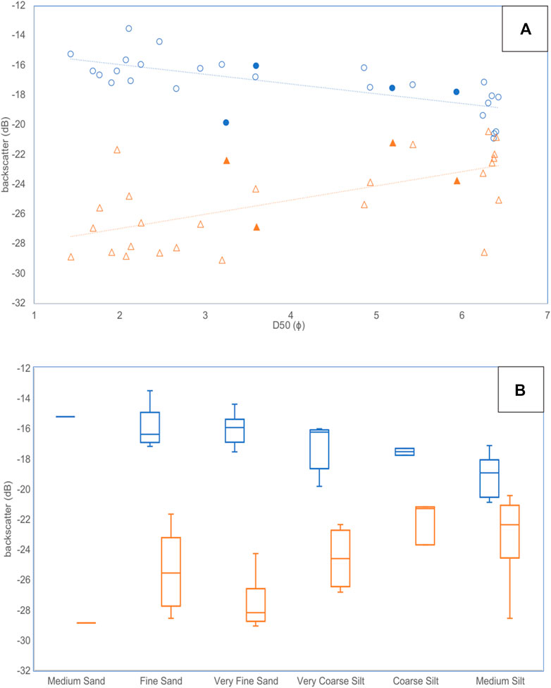
FIGURE 5. (A) 200 (blue circles) and 30 (orange triangles) kHz backscatter values and D50 (median ϕ) particle size. All South Calypso HVF samples are highlighted within the black rectangle, where ϕ > 6.0 (smallest median particle sizes). Infilled icons indicate samples from the two depressions in the North Calypso HVF. (B) 200 (blue) and 30 (orange) kHz backscatter intensity and Folk & Ward sediment classification. All South Calypso HVF samples are medium silt, highlighted within the black rectangle. Here, there is minimal overlap in range between 200 and 30 kHz mosaic backscatter values.
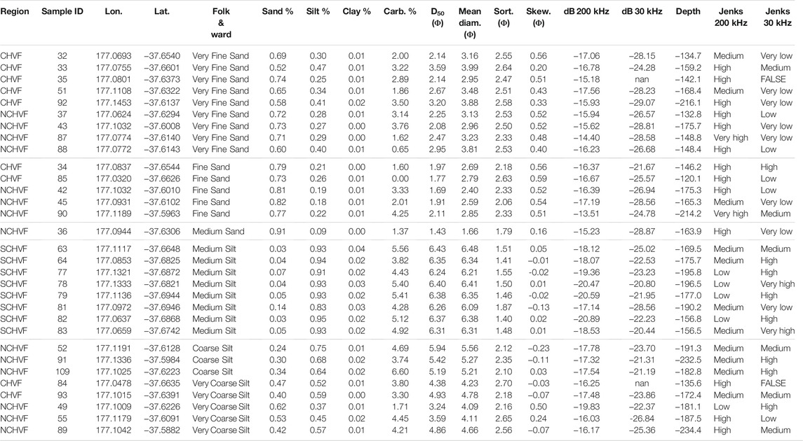
TABLE 2. Sediment grab Folk and Ward classes, composition, and corresponding Jenks Natural Breaks acoustic classes for both mosaics.
Backscatter Segmentation
All 200 kHz-derived GEOBIA segments and most of the 30 kHz-derived and combined mosaic GEOBIA segments have irregular shapes for all SPs, aligning with observed natural features in both the bathymetry and backscatter (subsets shown in Figure 6 show SP46 for the NCHVF and SP75 for the SCHVF, the two best performing models for each region). Segments that do not align with natural features within the 30 kHz or combined segmentation are due to artefacts in the mosaics (i.e. predominantly artefacts that are a result of aeration of the transducer due to rough sea conditions).
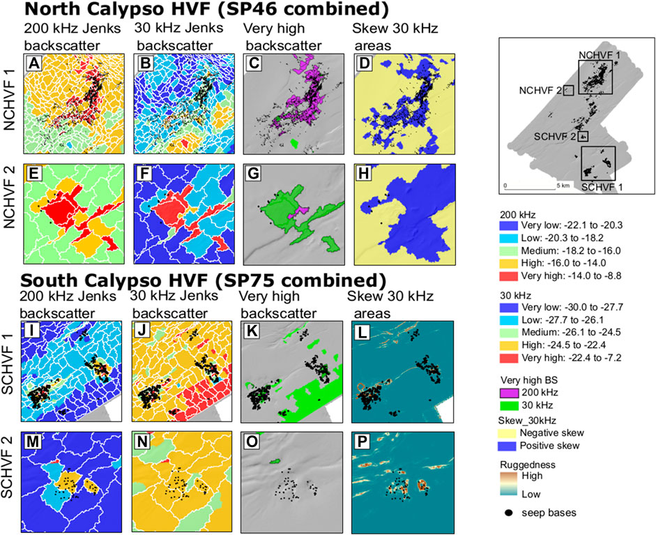
FIGURE 6. Seeps (black dots), segmentation (white lines), and Jenks Natural Breaks re-classification of segments (colours) based on distribution of mean backscatter levels. Row names refer to location on inset map. First two rows (A-H) show North Calypso HVF subsets of the segmentation with SP46 (the best performing NCHVF model); bottom two rows (I-P) show South Calypso HVF subsets of the segmentation with SP75 (the best performing SCHVF model). First column (A,E,I,M) shows Jenks classes of mean 200 kHz backscatter values. Second column (B,F,J,N) shows segment Jenks classes of mean 30 kHz backscatter values. Third column (C,G,K,O) shows comparison of very-high backscatter segments of the 200 kHz (purple with black outline) and 30 kHz (green) segments, with other segments removed. Green (30 kHz) segments with a dark outline are overprinted 200 kHz very-high segments. Top of fourth column (D,H) show segments with mean negative (cream segments) and positive (navy segments) skew of the 30 kHz mosaic, the most important variable in the North Calypso HVF best performing model. Bottom of fourth column (L,P) show the vector ruggedness measure (rugosity) bathymetric derivative layer, overlain by seeps, the most important variable in the South Calypso HVF best performing model.
As SP increased, segments that delineate very-high backscatter areas remained mostly stable while segments that delineate homogenous areas of seafloor increased in size (Figure 6). Segments that delineate scarps also remain stable at higher SP levels (Figures 6E,F,I,J). Though the ESP2 tool provides a repeatable and objective method for selecting SPs, we found the chosen SPs did not adequately identify boundaries of the hardground areas. Smaller SPs (SP9, SP14, and SP26), resulted in over segmentation, where too many segments were created without delineating conspicuous natural boundaries of features. These SPs resulted in highly granular segments, demarcating contiguous very-high backscatter areas into small segments.
Prediction Model Results for Seep Presence
Due to the imbalance of examples between “active” and “inactive” areas (Section 3.8) standard model accuracy levels give a poor representation of “goodness” as the models correctly predict “inactive” areas far better than “active” areas. Of the 63 models run in this study, three were considered good, with Kappa >0.6 (Altman, 1991). These ‘good’ models were all North Calypso HVF (NCHVF) combined mosaic models, with SP 46, 75, and 50 (Table 3). NCHVF04 (combined mosaics, SP 46, accuracy: 0.75), with the highest Kappa value of 0.65, performed significantly better than the individual mosaic models with equivalent SP (Figure 10). NCHVF04 had a 0.15 Kappa increase over NCHVF18 (30 kHz, SP46, Kappa: 0.50, accuracy: 0.77) and ∼0.20 over NCHVF11 (200 kHz, SP46, Kappa: 0.45, accuracy: 0.75).
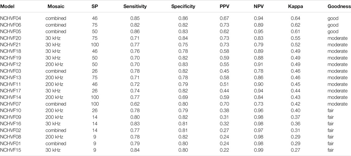
TABLE 3. North Calypso HVF random forest results ordered by Kappa score.
The second-best performing model, NCHVF06 (combined mosaic, SP75, accuracy: 0.82) had a lower Kappa (0.62) though higher PPV (0.73) than the best performing model, being better at predicting seep segments. NCHVF05, the third “good” model, had highest overall accuracy (0.84) but lower Kappa (0.61) and lower PPV (0.62). The NCHVF12 model (30 kHz mosaic, SP100, Kappa: 0.52) had the highest PPV of 0.73 and NPV of 0.79. Of the SP levels selected by the ESP tool, only SP46 revealed a good model relationship.
The combined mosaic model with SP 75 (Table 4) was the best performing model for the South Calypso HVF (SCHVF) (SCHVF06; Kappa: 0.57, “moderate,” accuracy: 0.81); this was also the model with highest PPV (0.61) (Figure 10). We found no significant difference between the combined model or the individual mosaic models with equivalent SP: SCHVF20 (30 kHz, SP75, Kappa: 0.56, accuracy: 0.85) and SCHVF13 (200 kHz, SP75, Kappa: 0.55, accuracy: 0.85), the second and third best performing models, respectively, for the South Calypso HVF. Of the SP levels selected by the ESP tool, none revealed a good model relationship.
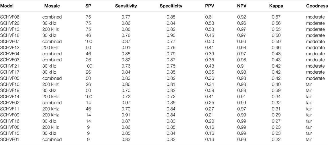
TABLE 4. South Calypso HVF random forest results ordered by Kappa score.
The CHVF20 30 kHz mosaic model with SP 75 (Table 5) was the best performing model for the full Calypso HVF, incorporating all data including artefacts (Kappa: 0.51, “moderate,” accuracy: 0.86). The best performing model for predicting seeps, with a PPV of 0.54, was CHVF07 (combined mosaics, SP100, Kappa: 0.50, accuracy: 0.79), the second-best performing model for the full Calypso HVF. All the SP levels selected by the ESP tool (SP14, SP26, and SP46) were ranked as ‘fair’ models.
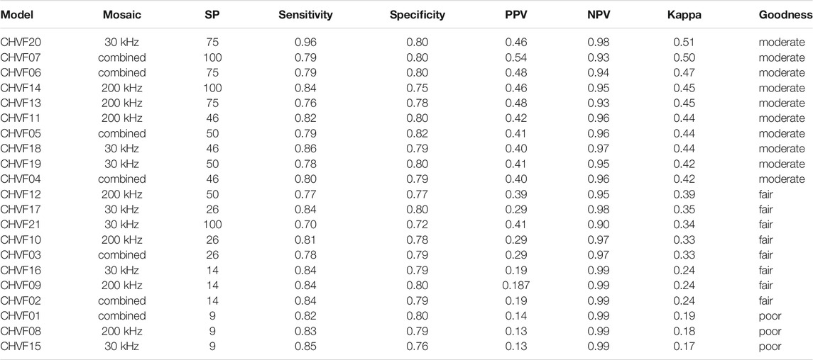
TABLE 5. Full Calypso HVF random forest results ordered by Kappa score.
Hardgrounds and Correctly Predicted Seep Presence
By applying a Jenks Natural Breaks classification to the updated distribution of mean backscatter values for each mosaic (moving from a pixel-based distribution to a segment-based distribution) we determined where high or very-high backscatter areas (“hardgrounds”) are in the Calypso HVF and how they may correlate with water column acoustic flares (“active fluid expulsion”).
For the best performing model, NCHVF04 (North Calypso HVF, combined mosaics, SP46), only 1.5% (0.51 km2) of the total area has very-high backscatter values in the 200 kHz mosaic (−14.0 to −8.8 dB) while 5.8% (1.94 km2) of the total area has very-high backscatter values in the 30 kHz mosaic (−2.4 to −7.2 dB) (Figure 10C).
Of the very-high 200 kHz backscatter segments, 0.3 km2 (0.87% of the total North Calypso HVF area) were also true positives (i.e. correctly predicted active fluid expulsion segments) while 0.2 km2 (0.67% of the total North Calypso HVF area) were false positives (i.e. incorrectly predicted active fluid expulsion) segments. Of the very-high 30 kHz backscatter segments, only 0.07 km2 were true positives; 1.37 km2 were false positives (Figure 10C). The remainder comprised true negatives and false negatives.
Predictor Variable Importance
The nine most important predictor variables for the best performing model, NCHVF04 (combined 30 and 200 kHz, SP46), include a combination of backscatter and bathymetric derived variables (Figure 7A). Skewness of 30 kHz, the distribution asymmetry of backscatter values from the pixels that construct a segment, has the highest relative importance to all other variables, meaning this variable would have the most negative impact on the model accuracy if removed. Segments with positive skew (segments that were made up of a majority of low mean dB values with a few very-high values in the tail, i.e. areas of soft sediment with flares) were aligned with areas that contained known seeps, (Figures 6D,H). Ruggedness and slope were the next most important predictor variables for NCHVF04. Mean EM2040 backscatter values (i.e. mean 200 kHz values that contribute to each segment) was the fifth most important variable. For the second-best performing model, NCHVF06, skewness of 30 kHz was the most important variable while it was third most important for the third best model NCHVF05.
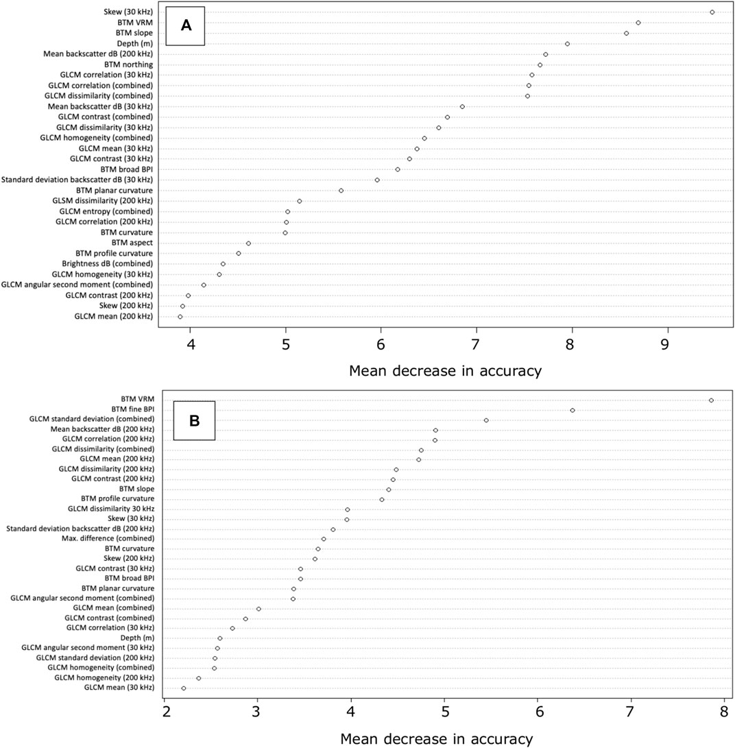
FIGURE 7. Variable importance plots of the “mean decrease in accuracy” measure. (A) North Calypso HVF best performing model NCHVF04: combined mosaics, SP46; (B) South Calypso HVF best performing model SCHVF06: combined mosaics, SP75.
The seven most important predictor variables for model SCHVF06 (combined 30 and 200 kHz, SP75) were a combination of backscatter and bathymetric derived variables, with vector ruggedness measure the most important (Figures 6L,P, 7B). Ruggedness has the highest relative importance to all other variables, i.e. if removed, this variable would reduce the model accuracy the most. Fine bathymetric position index was the next most important variable. Skewness of the 30 kHz was 13th in relative importance for this model.
Seafloor Observations
Towed camera footage, though biased toward discrete seafloor areas of interest, provides additional information about active seafloor fluid expulsion that accords with model results. Though not spatially extensive, video footage confirms the assumption that very-high backscatter classes are due to indurated or lithified seafloor. Carbonate platforms and lithified seafloor observed in the towed camera aligned with high and very-high backscatter areas observed in the mosaics (Figure 8). This relationship was more obvious however in the 30 kHz mosaic and for FOI-02 and -03 (Figures 8D,E, 9). No shell hash, mussel beds, or other potential reflectors traditionally also associated with fluid expulsion zones, and potential causes of high seafloor backscatter, where observed in the video footage. FOI-01 in the North Calypso HVF (Figures 8A,B) exhibits a high intensity of fluid expulsion coinciding with bioturbated sediment (Figure 9.1-3). Videos show shimmery fluid (due to density differences) escaping from the perimeters of anhydrite mounds (∼1 m diameter) covered in white filamentous bacteria (Figure 9.4-6); less intensive bubble expulsion was also observed. This fluid expulsion coincided with very-high backscatter in the 200 kHz mosaic (Figure 8A) and broadly low backscatter with smaller patches of very-high backscatter in the 30 kHz mosaic (Figure 8B).
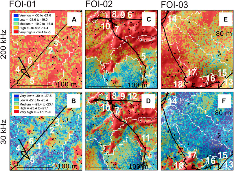
FIGURE 8. Towed camera transects (black lines) for three features of interest (FOI; see Figure 1B for locations) mapped over 200 kHz mosaic (A,C,E) and 30 kHz mosaic (B,D,E) show a variety of substrates both with and without active fluid expulsion. Black dots - seep base locations; mosaic resolution 2 m; projection NZTM; white lines: segments of best performing models for North (SP46 combined) and South (SP75 combined). Numbers correspond to still images in Figure 9.
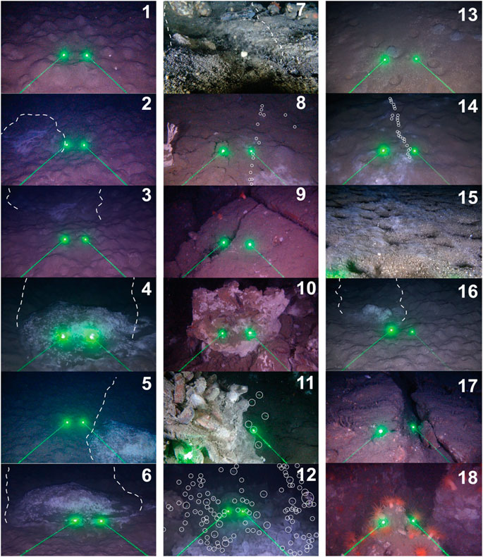
FIGURE 9. Still images for three features of interest (FOI; see Figure 1B for FOI locations). Numbers correspond to approximate locations along towed camera transects in Figure 8. White dashed lines highlight where fluid was observed exiting the seafloor; white circles highlight observable bubbles.
FOI-02 in the South Calypso HVF (Figures 8C,D) hosted a wide variety of substrates: sedimented regions with high-flux fluid expulsion (Figure 9.7); bioturbated sediment (as evidenced by active burrowing within surface sediment) with gas expulsion (Figure 9.8); hardground regions with low-flux fluid expulsion from the perimeters of, or in between, broken platforms (Figure 9.9) or rocky piles of hardgrounds (Figure 9.10); occasional anemone gardens (Figure 9.9) and mussel beds (Figure 9.10); areas of extensive white filamentous bacterial mats with very-high-flux gas and liquid expulsion (Figure 9.11). Of note were the many instances of liquid and gas bubble expulsion at the same area of seabed, with one high flux gas and fluid expulsion area of rocky substrate blanketed by thick white bacterial mats (Figure 9.12). These hardground regions coincided with very-high backscatter intensity in both mosaics. Other very-high backscatter intensity patches in the South Calypso HVF survey area were not sampled with the towed camera.
FOI-03 in the North Calypso HVF (Figures 8E,F), hosts fluid expulsion coinciding with a broad break of slope (Figure 1B). This seafloor was characterized by: bioturbated sedimented regions with no fluid expulsion (Figure 9.13); white and lilac colored filamentous bacterial with and without gas bubble expulsion (Figure 9.14), with lilac colored bacteria corresponding with areas of minimal fluid expulsion (Figure 9.15); ∼0.5 m diameter anhydrite mounds with high flux liquid expulsion (observed in towed camera footage as shimmery film) (Figure 9.16); hardground regions with lower flux gas bubble expulsion, from the perimeters of, or in between, broken platforms (Figure 9.17) and rocky piles of hardgrounds; and occasional anemone gardens (Figure 9.18). Here, hardground areas corresponded to very-high backscatter intensity in the 30 kHz mosaic and also in the 200 kHz mosaic, though the overall very-high intensity signal of the 200 kHz mosaic obscured direct comparisons between very-high 200 kHz values and seafloor observations. More extensive and very-high backscatter intensity patches in the North Calypso HVF survey area were not sampled with the towed camera on this survey.
Discussion
Quantitative Links Between Active Seepage and Seafloor Characteristics
We were able to link water-column acoustic flares (as an active fluid expulsion proxy) to specific backscatter and bathymetric derivatives of the seafloor using RF models at a shallow hydrothermal vent field. The best performing model (North Calypso HVF, combined mosaics, SP46, with overall accuracy: 0.75; PPV: 0.67; Kappa accuracy: 0.65) demonstrated the potential of using GEOBIA analysis, image segmentation, and RF modelling to predict regions of potential fluid expulsion based on seafloor characteristics (Figure 10). Although the South Calypso models were not as accurate, they still performed well in highlighting areas where active fluid expulsion were observed (Figure 10).
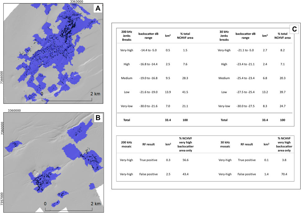
FIGURE 10. Final model predictions for the best performing models of (A) North Calypso HVF (SP46) and (B) South Calypso HVF (SP75) with seep locations (black dots) overlain, alongside (C) segment area and very-high backscatter area confusion matrix results for the best performing NCHVF model.
We were unable however to link gas flares specifically to “hardgrounds,” or very-high backscatter areas. Although areas of very-high backscatter areas in the 200 kHz mosaic were associated with predicted seep locations in the North, very-high backscatter dominated the whole mosaic most likely due to sand-dominant seafloor surface substrate overprinting discrete hardground areas, including areas that lacked seeps (Figure 8A). This finding contradicted what was observed in the 30 kHz mosaic, with seeps associated with a range of backscatter values, from low to very-high. These results however, combined with those provided by the RF variable importance measure, provide us with initial seafloor indicators associated with active fluid expulsion.
Naudts et al. (2008) observed that while fluid expulsion activity from shallow (<200 m water depth) seeps in the NW Black Sea and “hardground” backscatter were often correlated, higher fluid expulsion occurred adjacent to, or nearby, these hardgrounds. Along the Hikurangi Margin Naudts et al. (2010) noted that fluid expulsion from seeps in water deeper than 500 m escaped from sandy sediments away from highly reflective backscatter hardground platforms. Mitchell et al. (2018) however, supported the intuitive link between gas flares and potential hardgrounds when superimposing water column acoustic flares over anomalous seafloor backscatter intensities from ∼1,000 to 2000 m in the Gulf of Mexico. Thorsnes et al. (2019) showed on the Norwegian continental shelf (<400 m) that spatial relationships between hardgrounds and seeps are not always consistent, particularly when considering relict or dormant systems, or for fluid expulsion systems occurring from seafloor with more highly variable substrate types.
Implications for Predictive Modelling of Active Fluid Expulsion
Whilst we demonstrate from this example that areas of very-high seafloor backscatter are not good predictors of gas flares in this context, we suggest finer-scale textural indicators may be a useful tool to determine locations of active seeps. Skewness of the 30 kHz mosaic segments, whereby segments with positive skew were associated with known seeps, was the most influential variable in the best performing model and ranked highly in most of the other models. Positive skew describes the long-tailed distribution of all the 30 kHz pixels that contribute to each segment, with a higher density of relatively lower pixel values with few much higher values (the positive tail). This corresponds to textures observable in the 30 kHz mosaic, for e.g. Figure 8B, where discrete patches of high to very-high backscatter values are scattered among surrounding lower backscatter values.
Towed camera footage shows a similar relationship—areas of rubble or broken hardgrounds with minimal to no fluid flux were interspersed with unconsolidated sediment that hosted the most ebullient seeps (Figure 9). Although we found smaller SPs did not contribute to any of the best performing models, segment skewness may more aptly capture the fine-scale seafloor textures that are lost when using segmentation and GEOBIA methods, while still allowing for noise inherent in seafloor backscatter mosaics to be accounted for.
A Combined Frequency Approach to Improve Model Accuracy
Results from the Calypso HVF demonstrate that combining backscatter mosaics from multiple frequencies increased model accuracy compared to using individual mosaics. The combined models were the best performers for both the North and South Calypso HVFs. We suggest the improved predictive power, compared to a single frequency, is achieved by capturing information from both surface backscatter and notable acoustic returns in the immediate sub seafloor surface. Buscombe and Grams (2018) suggested that increasing dimensionality in a seafloor classification, by using multiple frequency mosaics, provides more points of understanding for a model to draw upon when determining substrate boundaries. Classification models using the single 30 kHz mosaics for North and South also outperformed their equivalent 200 kHz-based models at each of the segmentation scales, both in overall model accuracy and predictive power. In the North in particular, the 30 kHz mosaic better highlights areas of very-high to high backscatter than the 200 kHz, as there is difficulty differentiating between sandy substrate and hardgrounds in the higher frequency mosaic using backscatter alone (Figure 4C). Sand grains (<4 ϕ), as observed in the sediment samples collected in the North Calypso HVF, are strong acoustic scatterers, comparable to hard substrate (Lurton and Lamarche, 2015). The lower frequency sounder was able to penetrate beneath the sandy overprinting veneer and better delineate the hardgrounds beneath. Work has been undertaken to estimate signal penetration depths, with low frequency systems having the greatest penetration potential: e.g. 4 m (Hillman et al., 2017) or 12 m (Schneider Von Deimling et al., 2013) penetration for a 12 kHz signal; up to 7 m penetration for 27–30 kHz (Mitchell, 1993), and decimeter penetration for a 95 kHz signal (Fonseca et al., 2002). This demonstrates the usefulness of employing a lower frequency sounder than would typically be considered ideal for these depth ranges (<200 m) to reveal sub-surface structures.
The usefulness of using a lower frequency sounder, or combining two frequency sounders, for classifying the seafloor and interpreting sediment at depth has been demonstrated elsewhere. Hughes Clarke (2015) initially demonstrated that so long as a minimum separation of one octave between frequencies is maintained, two discrete MBES frequencies may enable frequency differences to be exploited and allow for improved discrimination between surface seafloor characteristics and subsurface information. Gaida et al. (2018) found that using a 100 and 400 kHz combination increased substrate discrimination in the Bedford Basin, Canada, compared with using a single frequency. Working on the same dataset, Brown et al. (2019), observed coarse sub-surface dredge spoils in a 100 kHz mosaic that were not observed in the 400 kHz mosaic. Feldens et al. (2018) found that lower frequency data were more sensitive to substrate changes, highlighting buried seafloor structures that were not detected in higher frequency data and highlighted the greatest contrast between seafloor facies. This allowed for additional sediment classes to be produced by combining surface acoustic information with subsurface acoustic information observed in the 100 kHz frequency backscatter data. Buscombe and Grams (2018) showed that multi-spectral data and spatially-aware machine learning algorithms that do not rely on assumptions of independence in substrate models may better determine substrate classifications. Janowski et al. (2018) however, highlighted that multi-spectral seafloor mosaics, though ideal, are not always required for seafloor discrimination. They showed a frequency pair (150 and 400 kHz) can provide enough additional frequency information to improve overall accuracy of RF models. Specific to shallow hydrothermal vent fields, penetrative backscatter differences may be useful in detecting emergent seeps or sub-surface sediment modification or classes that are difficult to detect from a conventional single frequency mapping approach, while spatially-aware machine learning algorithms may allow for the incorporation of broader geological influences such as fault scarps.
Factors Affecting Model Accuracy
We propose differences in model accuracy between the North and South Calypso HVF are the result of two different seep settings, both in surrounding substrate and seep style, and may imply two distinct or diverging seep systems. We also speculate that a complex arrangement of precipitated minerals, including hydrothermal sulfates (e.g. anhydrites) as well as carbonates, may be producing the very-high seafloor backscatter anomalies at the seafloor surface of the two sites. Overprinting by terrigenous and volcanic sediments may also affect model accuracy due to hardground burial however sedimentation rates in the Bay of Plenty, in particular the Calypso site are relatively low (in the order of decimeters per 10,000 years) (Kohn and Glasby, 1978; Bostock et al., 2018).
The South Calypso HVF seeps are represented by the very-high backscatter mounds surrounded by medium silt seafloor (predominantly low backscatter in the 200 kHz and medium in the 30 kHz mosaic). The North Calypso HVF in contrast exhibits a constellation of seeps over varying substrate types. The South Calypso HVF is nearer to the Whakatāne Graben axis than the North and noticeably, the South Calypso HVF seep clusters exhibit more ebullient liquid and gas flux in video footage than what we observed in the North. This nearness of the South Calypso HVF to the graben axis, its more active appearance, and more discrete emplacement style lacking extensive hardgrounds may imply a younger hydrothermal seep than the North. In addition, a higher abundance of gas at depth in the South Calypso HVF sediments may contribute to the higher intensity response observed in the 30 kHz mosaic. The relatively lower gas flux, compared to the South, and extensive sediment settling on most of the hardground platforms observed in the towed camera suggest the North hardground areas are less active and have been emplaced over a longer period of time (thousands of years) (Bowden et al., 2013). The combined extensive hardgrounds and active seeps in the North suggest a combined seep system of active hydrothermal venting and longer-lived carbonate hardgrounds. Largely, the emplaced hardgrounds closely resemble authigenic carbonate platforms observed at cold methane seeps, implying a gentler hydrothermal gradient with the potential to encourage microbial anaerobic oxidation of methane to occur.
Procesi et al. (2019) pose that the Calypso HVF is a sediment-hosted geothermal system (SHGS). SHGSs are geological vent and seep systems that straddle both strictly hydrothermal and hydrocarbon arrangements; they emit both mantle derived CO2 and biotic CH4. For Calypso HVF, Stoffers et al. (1999) and Kamenev et al. (1993) both reported the presence of hydrocarbons in vent fluid and bottom waters. Botz et al. (2002) measured 83.61% CO2 and 6.196% CH4 within the North Calypso HVF vent gas, with a temperature of 201°C. Values of 72.10% CO2 and 9.898% CH4 in vent gas and 51.79% CO2 and 1.182% CH4 in vent water, with a temperature of 181°C recorded at the South Calypso HVF. While the carbon isotope values observed between −3.4‰ and −5.5‰ of the reference standard for δ13C (Pee Dee Belemnite (PDB)) indicate a shallow magmatic source for the CO2 gas, δ13C isotope values between −24.6‰ and -28.9‰ PDB at Calypso HVF also indicate CH4 sourced from thermal maturation of organic matter (thermogenesis) within marine sediments (Botz et al., 2002).
Sarano et al. (1989) and Kamenev et al. (1993) reported anhydrite mounds up to 8 m in height. Numerous smaller (∼1–2 m high) anhydrite mounds, with observable liquid escape (shimmery water-column features in the video footage) and associated filamentous bacteria, were observed during the 2018 voyage. No mounds were detected on the same scale as the previously observed mound (Figure 9). The small anhydrite mounds observed during the 2018 voyage may be a precursor to larger cones, if the vent pathway is maintained, or eroded versions of formerly larger features. Hocking et al. (2010) observed that the largest mound had visibly eroded over two decades, suggesting high temperature fluid expulsion may have waned or relocated in the North Calypso HVF since original observations were made by Sarano et al. (1989). Anhydrite forms as hot calcium-rich hydrothermal fluids mix with cold sulfate-rich sea water (Sarano et al., 1989; Hannington et al., 2001; Lowell et al., 2003). The retrograde solubility for anhydrite is > 150°C; below this threshold, anhydrite dissolves (Mottl, 1983). Without a constant supply of hot vent fluid, anhydrite dissolves at shallow depths (<200 m) (Lowell and Yao, 2002; Lowell et al., 2003). Hardgrounds however exist on timescales many orders of magnitude longer than active fluid expulsion (Bayon et al., 2009; Liebetrau et al., 2010; Bowden et al., 2013); coexistent hardgrounds and anhydrite mounds suggest both long-lived and contemporary fluid expulsion. Consequently, modelling flares to hardgrounds may not capture such timescale differences.
Improvements and Future Applications
Fine tuning our approach may lead to more sophisticated means of locating and differentiating between active and relict fluid expulsion areas. Additional recommendations for future mapping might consider the following elements in each step of the modeling pathway.
Acquisition
A stratified random sampling regime, combined with more extensive video footage to observe first order indications of active and inactive fluid expulsion, would allow more robust associations between gas flares/fluid expulsion and seafloor characteristics. This would allow the unique seafloor textural differences associated with both to be captured and fully modeled. A single-pass survey using an integrated multi-spectral system for multi-frequency seafloor analysis (Brown et al., 2019) would ensure MBES calibration, correction, and data reduction issues could be reduced by collecting varying frequency information on a ping-by-ping basis. Further, repeat surveys to capture change detection in both the seafloor and water column acoustic backscatter would allow us to integrate short time frame fluctuations in a dynamic seep system into the model.
Processing
Seep identification using higher frequency (200 kHz) water-column acoustic data would allow us to interrogate more forms of fluid expulsion. We identified fluid expulsion using 30 kHz water-column acoustic data which favors gas expulsion. Additional fluid expulsion evidence may be found in the 200 kHz water-column data, e.g. liquid expulsion that lacks a gas fraction. Image segmentation and pre-classification could also be used to remove obvious artefacts prior to segmentation.
Modelling
Sampling hardground platforms in both regions, to determine sediment mineralogy, combined with acoustic information, discrete camera sampling, and geochronology could be used to determine the genesis or timescales of the active fluid expulsion regions. Additionally, seep differences could be modeled to further understand seafloor modifications possible within of a sediment-hosted geothermal system.
Conclusion
We demonstrate that a dual frequency approach, within the bounds of a MBES survey, leads to improved seep prediction. Combining the penetration and resolution of two distinct MBES frequencies can provide added value for the interpretation of seafloor structure from backscatter data. Understanding the potential of different acoustic frequencies when targeting specific seafloor substrates is necessary to inform decisions of vessel choice or limitations when preparing for a survey of a key substrate type. We show that extensive and precise ground-truthing (through video, grabs, and cores) that enable strong associations between paired or multi-frequency seafloor maps are required to advance our understanding of penetration depth and influence of sounder choice on seafloor substrate classification. Understanding the limits imposed by chosen frequencies and sonar systems will increase these associations, while improving integration methods for paired frequency systems.
The main outcome of this study is that the extensive hardgrounds of the Calypso HVF are not directly linked with gas flares within this shallow hydrothermal system, while unconsolidated sediment nearby hosts higher flux expulsion. This aligns with the development and cessation of other submarine fluid expulsion system (Naudts et al., 2008; Judd and Hovland, 2009; Naudts et al., 2010). Seafloor fluid systems will refashion themselves on decadal timescales due to vent instability, clogging from deposited minerals, modification of the sediment, or rearrangement due to ongoing extensional processes and tectonic stresses (Desbruyères, 1998; Bowden et al., 2013; Levin et al., 2016). Once a seep self-seals, fluid will migrate to a more permeable pathway. Being able to remotely predict active and inactive regions of fluid expulsion will prove a useful tool in rapidly identifying seeps in legacy datasets, as well as textural metrics that will aid in locating nascent, senescent, or even extinct seeps during a survey, where important communities may persist even if they appear inactive. Understanding the seafloor qualities best able to predict active or inactive fluid expulsion will allow us to establish primary controls on fluid expulsion in a shallow marine environment and further understand seep succession stages and evolution.
Data Availability Statement
The raw data supporting the conclusion of this article will be made available by the authors, without undue reservation.
Author Contributions
All authors give final approval of the article to be published. ES conceived and designed the project; processed and analyzed data; generated segmentation and random forest analysis output; substantially drafted, constructed, and revised the article and figures. GL was voyage leader of QUOI-TAN1806 voyage that produced the data and was science leader of public funded program that funded the research. GL and VL funded the voyage from project “Building capability for in situ quantitative characterization of the ocean water-column using acoustic multibeam backscatter data” (2017–2018) - Royal Society of New Zealand Catalyst Fund. JW, VL, and GL supervised the project; provided analytical support and guidance; critically reviewed and revised the article. SW acquired and processed data; provided technical and analytical support; revised the article. YL acquired and processed data; provided technical support; revised the article. EH acquired and processed data; provided technical support; revised the article. AP acquired and processed data; provided technical support; revised the article.
Funding
ES is funded under the Australian Research Council’s Special Research Initiative for Antarctic Gateway Partnership (Project ID SR140300001). GL and VL were funded by The Royal Society of New Zealand Catalyst Fund project: “Building capability for in situ quantitative characterization of the ocean water-column using acoustic multibeam backscatter data (2017–2018)”. This research contributes to the Ministry of Business, Innovation, and Employment (MBIE) funded Smart Ideas Grant: “Broadband acoustic characterization of free gases in the ocean water (Contract C01X1915)” and is further supported by the MBIE Strategic Science Investment Fund (SSIF) Marine Geological Processes Program of the NIWA Coasts and Oceans Centre (COPR).
Conflict of Interest
The authors declare that the research was conducted in the absence of any commercial or financial relationships that could be construed as a potential conflict of interest.
Publisher’s Note
All claims expressed in this article are solely those of the authors and do not necessarily represent those of their affiliated organizations, or those of the publisher, the editors and the reviewers. Any product that may be evaluated in this article, or claim that may be made by its manufacturer, is not guaranteed or endorsed by the publisher.
Acknowledgments
We thank the captain, crew, and science team of the RV Tangaroa QUOI/TAN1806 voyage. We also thank Yves Le Gonidec, Arnaud Gaillot (IFREMER); Tom Weber, Liz Weidner (UNH); Amy Nau (UTAS); Lisa Northcote (NIWA).
References
Augustin, J.-M. (2016). SonarScope ® Software On-Line Presentation. Available at: http://flotte.ifremer.fr/fleet/Presentation- of-the-fleet/On-board-software/SonarScope.
Bayon, G., Henderson, G. M., and Bohn, M. (2009). U-th Stratigraphy of a Cold Seep Carbonate Crust. Chem. Geology. 260, 47–56. doi:10.1016/j.chemgeo.2008.11.020
Blott, S. J., and Pye, K. (2001). GRADISTAT: a Grain Size Distribution and Statistics Package for the Analysis of Unconsolidated Sediments. Earth Surf. Process. Landforms 26, 1237–1248. doi:10.1002/esp.261
Bostock, H., Jenkins, C., Mackay, K., Carter, L., Nodder, S., Orpin, A., et al. (2018). Distribution of Surficial Sediments in the Ocean Around New Zealand/Aotearoa. Part B: continental Shelf. New Zealand J. Geology. Geophys. 62, 24–45. doi:10.1080/00288306.2018.1523199
Botz, R., Wehner, H., Schmitt, M., Worthington, T. J., Schmidt, M., and Stoffers, P. (2002). Thermogenic Hydrocarbons from the Offshore Calypso Hydrothermal Field, Bay of Plenty, New Zealand. Chem. Geology. 186, 235–248. doi:10.1016/s0009-2541(01)00418-1
Bowden, D. A., Rowden, A. A., Thurber, A. R., Baco, A. R., Levin, L. A., and Smith, C. R. (2013). Cold Seep Epifaunal Communities on the Hikurangi Margin, New Zealand: Composition, Succession, and Vulnerability to Human Activities. PLoS One 8, e76869. doi:10.1371/journal.pone.0076869
Brown, C. J., Beaudoin, J., Brisette, M., and Gazzola, V. (2019). Multispectral Multibeam echo Sounder Backsactter as a Tool for Improved Seafloor Characterization. Geosciences 9, 1–19. doi:10.3390/geosciences9030126
Buscombe, D., and Grams, P. (2018). Probabilistic Substrate Classification with Multispectral Acoustic Backscatter: A Comparison of Discriminative and Generative Models. Geosciences 8, 1–21. doi:10.3390/geosciences8110395
Buscombe, D. (2017). Shallow Water Benthic Imaging and Substrate Characterization Using Recreational-Grade Sidescan-Sonar. Environ. Model. Softw. 89, 1–18. doi:10.1016/j.envsoft.2016.12.003
Canet, C. (2003). Methane-related Carbonates Formed at Submarine Hydrothermal Springs: a New Setting for Microbially-Derived Carbonates? Mar. Geology. 199, 245–261. doi:10.1016/s0025-3227(03)00193-2
Conti, A., D’emidio, M., Macelloni, L., Lutken, C. B., Asper, V., Woolsey, M., et al. (2016). “Morpho-acoustic Characterization of Natural Seepage Features Near the Macondo Wellhead (ECOGIG Site OC26, Gulf of Mexico). in” Deep Sea Research II. doi:10.1016/j.dsr2.2015.11.011
Desbruyères, D. (1998). Temporal Variations in the Vent Communities on the East Pacific Rise and Galápagos Spreading Centre: a Review of Present Knowledge. Cah. Biol. Mar. 39.
Dragut, L., Tiede, D., and Levick, S. R. (2010). ESP: a Tool to Estimate Scale Parameter for Multiresolution Image Segmentation of Remotely Sensed Data. Int. J. Geographical Inf. Sci. 24, 859–871. doi:10.1080/13658810903174803
Duncan, A. R., and Pantin, H. M. (1969). Evidence for Submarine Geothermal Activity in the Bay of Plenty. New Zealand J. Mar. Freshw. Res. 3, 602–606. doi:10.1080/00288330.1969.9515322
Feldens, P., Schulze, I., Papenmeier, S., Schönke, M., and Schneider Von Deimling, J. (2018). Improved Interpretation of marine Sedimentary Environments Using Multi-Frequency Multibeam Backscatter Data. Geosciences 8, 1–14. doi:10.3390/geosciences8060214
Finkl, C. W., and Makowski, C. (2016). Seafloor Mapping along continental Shelves: Research and Techniques for Visualizing Benthic Environments. Switzerland: Springer.
Folk, R. L., and Ward, W. C. (1957). Brazos River Bar [Texas]; a Study in the Significance of Grain Size Parameters. J. Sediment. Res. 27, 3–26. doi:10.1306/74d70646-2b21-11d7-8648000102c1865d
Fonseca, L., Mayer, L., Orange, D., and Driscoll, N. (2002). The High-Frequency Backscattering Angular Response of Gassy Sediments: Model/data Comparison from the Eel River Margin, California. The J. Acoust. Soc. America 111, 2621–2631. doi:10.1121/1.1471911
Gaida, T., Tengku Ali, T., Snellen, M., Amiri-Simkooei, A., Van Dijk, T., and Simons, D. (2018). A Multispectral Bayesian Classification Method for Increased Acoustic Discrimination of Seabed Sediments Using Multi-Frequency Multibeam Backscatter Data. Geosciences 8, 1–25. doi:10.3390/geosciences8120455
Gentz, T., Damm, E., Schneider Von Deimling, J., Mau, S., Mcginnis, D. F., and schlüter, M. (2014). A Water Column Study of Methane Around Gas Flares Located at the West Spitsbergen continental Margin. Continental Shelf Res. 72, 107–118. doi:10.1016/j.csr.2013.07.013
Glasby, G. P. (1971). Direct Observations of Columnar Scattering Associated with Geothermal Gas Bubbling in the Bay of Plenty, New Zealand. New Zealand J. Mar. Freshw. Res. 5, 483–496. doi:10.1080/00288330.1971.9515399
Guillon, L., and Lurton, X. (2001). Backscattering from Buried Sediment Layers: The Equivalent Input Backscattering Strength Model. J. Acoust. Soc. America 109, 122–132. doi:10.1121/1.1329622
Hannington, M., Herzig, P., Stoffers, P., Scholten, J., Botz, R., garbe-Schönberg, D., et al. (2001). First Observations of High-Temperature Submarine Hydrothermal Vents and Massive Anhydrite Deposits off the north Coast of Iceland. Mar. Geology. 177, 199–220. doi:10.1016/s0025-3227(01)00172-4
Haralick, R. M., shanmugam, K., and Dinstein, I. H. (1973). Textural Features for Image Classification. IEEE Trans. Syst. Man. Cybern. SMC-3, 610–621. doi:10.1109/tsmc.1973.4309314
Hillman, J. I. T., Lamarche, G., Pallentin, A., Pecher, I. A., Gorman, A. R., and Schneider Von Deimling, J. (2017). Validation of Automated Supervised Segmentation of Multibeam Backscatter Data from the Chatham Rise, New Zealand. Mar. Geophys. Res. 39, 205–227. doi:10.1007/s11001-016-9297-9
Hocking, M. W. A., Hannington, M. D., Percival, J. B., Stoffers, P., Schwarz-Schampera, U., and De Ronde, C. E. J. (2010). Clay Alteration of Volcaniclastic Material in a Submarine Geothermal System, Bay of Plenty, New Zealand. J. Volcanology Geothermal Res. 191, 180–192. doi:10.1016/j.jvolgeores.2010.01.018
Huff, L. C. (2008). Acoustic Remote Sensing as a Tool for Habitat Mapping in Alaska Waters. Marine Habitat Mapping Technology for Alaska.
Hughes Clarke, J. E. H. (2015). “Multispectral Acoustic Backscatter from Multibeam, Improved Classification Potential,” in Proceedings of the United States Hydrographic Conference 2015 (San Diego, CA, USA.
Jackson, D. R., winebrenner, D. P., and ishimaru, A. (1986). Application of the Composite Roughness Model to High‐frequency Bottom Backscattering. J. Acoust. Soc. America 79, 1410–1422. doi:10.1121/1.393669
Janowski, L., Trzcinska, K., Tegowski, J., Kruss, A., Rucinska-Zjadacz, M., and Pocwiardowski, P. (2018). Nearshore Benthic Habitat Mapping Based on Multi-Frequency, Multibeam Echosounder Data Using a Combined Object-Based Approach: a Case Study from the Rowy Site in the Southern Baltic Sea. Remote Sensing 10, 1–21. doi:10.3390/rs10121983
Jenks, G. F. (1967). The Data Model Concept in Statistical Mapping. lnternational Yearb. Cartography 7, 186–190.
Jones, G. A., and Kaiteris, P. (1983). A Vacuum-Gasometric Technique for Rapid and Precise Analysis of Calcium Carbonate in Sediments and Soils. J. Sediment. Res. 53, 655–660. doi:10.1306/212f825b-2b24-11d7-8648000102c1865d
Judd, A. G., and Hovland, M. (2009). Seabed Fluid Flow: The Impact on Geology, Biology and the marine Environment. Northumberland, UK: Cambridge University Press.
Kamenev, G. M., Fadeev, V. I., Selin, N. I., Tarasov, V. G., and Malakhov, V. V. (1993). Composition and Distribution of Macro‐ and Meiobenthos Around Sublittoral Hydrothermal Vents in the Bay of Plenty, New Zealand. New Zealand J. Mar. Freshw. Res. 27, 407–418. doi:10.1080/00288330.1993.9516582
Kohn, B. P., and Glasby, G. P. (1978). Tephra Distribution and Sedimentation Rates M the Bay of Plenty, New Zealand. New Zealand J. Geology. Geophys. 21, 49–70. doi:10.1080/00288306.1978.10420721
Ladroit, Y., Lamarche, G., and Pallentin, A. (2017). Seafloor Multibeam Backscatter Calibration experiment: Comparing 45°-tilted 38-kHz Split-Beam Echosounder and 30-kHz Multibeam Data. Mar. Geophys. Res. 39, 41–53. doi:10.1007/s11001-017-9340-5
Lamarche, G., and Barnes, P. M. (2005). Fault Characterisation and Earthquake Source Identification in the Offshore Bay of PlentyNIWA Client Report. NIWA, Wellington: Prepared for Environment Bay of Plenty Regional Council.
Lamarche, G., Le Gonidec, Y., Lucieer, V., Ladroit, Y., Weber, T., Gaillot, A., et al. (2019). Gas Bubble Forensics Team Surveils the New Zealand Ocean. EOS 100, 1–10. doi:10.1029/2019eo133649
Lamarche, G., Lurton, X., Verdier, A.-L., and Augustin, J.-M. (2011). Quantitative Characterisation of Seafloor Substrate and Bedforms Using Advanced Processing of Multibeam Backscatter-Application to Cook Strait, New Zealand. Continental Shelf Res. 31, S93–S109. doi:10.1016/j.csr.2010.06.001
Levin, L. A., Baco, A. R., Bowden, D. A., Colaco, A., Cordes, E. E., Cunha, M. R., et al. (2016). Hydrothermal Vents and Methane Seeps: Rethinking the Sphere of Influence. Front. Mar. Sci. 3, 1–23. doi:10.3389/fmars.2016.00072
Levin, L. (2005). Ecology of Cold Seep Sediments. Oceanography Mar. Biol. Annu. Rev. 43, 1–46. doi:10.1201/9781420037449.ch1
Liebetrau, V., Eisenhauer, A., and Linke, P. (2010). Cold Seep Carbonates and Associated Cold-Water Corals at the Hikurangi Margin, New Zealand: New Insights into Fluid Pathways, Growth Structures and Geochronology. Mar. Geology. 272, 307–318. doi:10.1016/j.margeo.2010.01.003
Litchfield, N., Van Dissen, R., Sutherland, R., Barnes, P., Cox, S., Norris, R., et al. (2013). A Model of Active Faulting in New Zealand. New Zealand J. Geology. Geophys. 57, 32–56. doi:10.1080/00288306.2013.854256
Lowell, R. P., and Yao, Y. (2002). Anhydrite Precipitation and the Extent of Hydrothermal Recharge Zones at Ocean ridge Crests. J. Geophys. Res. Solid Earth 107. doi:10.1029/2001jb001289
Lowell, R. P., Yao, Y., and Germanovich, L. N. (2003). Anhydrite Precipitation and the Relationship between Focused and Diffuse Flow in Seafloor Hydrothermal Systems. J. Geophys. Res. Solid Earth 108, 1–8. doi:10.1029/2002jb002371
Lucieer, V., and Lamarche, G. (2011). Unsupervised Fuzzy Classification and Object-Based Image Analysis of Multibeam Data to Map Deep Water Substrates, Cook Strait, New Zealand. Continental Shelf Res. 31, 1236–1247. doi:10.1016/j.csr.2011.04.016
Lucieer, V. L., Hill, N. A., Barrett, N. S., and Nichol, S. (2012). Do marine Substrates ‘look’ and ‘sound’ the Same? Supervised Classification of Multibeam Acoustic Data Using Autonomous Underwater Vehicle Images. Estuarine, Coastal Shelf Sci., 1–13. doi:10.1016/j.ecss.2012.11.001
Lucieer, V. L. (2008). Object‐oriented Classification of Sidescan Sonar Data for Mapping Benthic marine Habitats. Int. J. Remote Sensing 29, 905–921. doi:10.1080/01431160701311309
Lurton, X., and Lamarche, G. (2015). Backscatter Measurements by Seafloor-Mapping Sonars: Guidelines and Recommendations. Plouzane, France: GEOHAB.
McGinnis, D. F., Greinert, J., Artemov, Y., Beaubien, S. E., and Wüest, A. (2006). Fate of Rising Methane Bubbles in Stratified Waters: How Much Methane Reaches the Atmosphere? J. Geophys. Res. 111, 1–15. doi:10.1029/2005jc003183
Medwin, H., and Clay, C. S. (1997). Fundamentals of Acoustical Oceanography. San Diego, CA: Academic Press.
Mellor, A., Boukir, S., Haywood, A., and Jones, S. (2015). Exploring Issues of Training Data Imbalance and Mislabelling on Random forest Performance for Large Area Land Cover Classification Using the Ensemble Margin. ISPRS J. Photogrammetry Remote Sensing 105, 155–168. doi:10.1016/j.isprsjprs.2015.03.014
Mitchell, G. A., Orange, D. L., Gharib, J. J., and Kennedy, P. (2018). Improved Detection and Mapping of deepwater Hydrocarbon Seeps: Optimizing Multibeam Echosounder Seafloor Backscatter Acquisition and Processing Techniques. Mar. Geophys. Res., 323–347 doi:10.1007/s11001-018-9345-8
Mitchell, J., Stevens, M., and Wilcox, S. (2004). RV Tangaroa TAN0412 Voyage Report: Bay of Plenty Swath and Hawke Bay Seismics. Unpublished Voyage Report. Wellington: NIWA.
Mitchell, N. C. (1993). A Model for Attenuation of Backscatter Due to Sediment Accumulation and its Application to Determine Sediment Thicknesses with GLORIA Sidescan Sonar. J. Geophys. Res. 98, 477–493. doi:10.1029/93jb02217
Monecke, T., Petersen, S., and Hannington, M. D. (2014). Constraints on Water Depth of Massive Sulphide Formation: Evidence from Modern Seafloor Hydrothermal Systems in Arc-Related Settings. Econ. Geology. 109, 2079–2101. doi:10.2113/econgeo.109.8.2079
Mottl, M. J. (1983). Metabasalts, Axial hot springs, and the Structure of Hydrothermal Systems at Mid-ocean Ridges. Geol. Soc. America Bull. 94, 164–180. doi:10.1130/0016-7606(1983)94<161:mahsat>2.0.co;2
Naudts, L., Greinert, J., Artemov, Y., Beaubien, S. E., Borowski, C., and batist, M. D. (2008). Anomalous Sea-Floor Backscatter Patterns in Methane Venting Areas, Dnepr paleo-delta, NW Black Sea. Mar. Geology. 251, 253–267. doi:10.1016/j.margeo.2008.03.002
Naudts, L., Greinert, J., Poort, J., Belza, J., Vangampelaere, E., Boone, D., et al. (2010). Active Venting Sites on the Gas-Hydrate-Bearing Hikurangi Margin, off New Zealand: Diffusive- versus Bubble-Released Methane. Mar. Geology. 272, 233–250. doi:10.1016/j.margeo.2009.08.002
Noé, S., Titschack, J., Freiwald, A., and Dullo, W.-C. (2006). From Sediment to Rock: Diagenetic Processes of Hardground Formation in Deep-Water Carbonate mounds of the NE Atlantic. Facies 52, 183–208. doi:10.1007/s10347-005-0037-x
Pantin, H. M., and Wright, I. C. (1994). Submarine Hydrothermal Activity within the Offshore Taupo Volcanic Zone, Bay of Plenty continental Shelf, New Zealand. Continental Shelf Res. 14, 1411–1438. doi:10.1016/0278-4343(94)90083-3
Phrampus, B. J., Lee, T. R., and Wood, W. T. (2020). A Global Probabilistic Prediction of Cold Seeps and Associated SEAfloor FLuid ExpulsionAnomalies (SEAFLEAs). Geochem. Geophys. Geosystems 21, 1–16. doi:10.1029/2019gc008747
Procesi, M., Ciotoli, G., Mazzini, A., and Etiope, G. (2019). Sediment-hosted Geothermal Systems: Review and First Global Mapping. Earth-Science Rev. 192, 529–544. doi:10.1016/j.earscirev.2019.03.020
Prol-Ledesma, R. M., Canet, C., Torres-Vera, M. A., Forrest, M. J., and Armienta, M. A. (2004). Vent Fluid Chemistry in Bahía Concepción Coastal Submarine Hydrothermal System, Baja California Sur, Mexico. J. Volcanology Geothermal Res. 137, 311–328. doi:10.1016/j.jvolgeores.2004.06.003
Reeburgh, W. S. (2007). Oceanic Methane Biogeochemistry. Chem. Rev. 107, 486–513. doi:10.1021/cr050362v
Römer, M., Wenau, S., Mau, S., Veloso, M., Greinert, J., Schlüter, M., et al. (2017). Assessing marine Gas Emission Activity and Contribution to the Atmospheric Methane Inventory: A Multidisciplinary Approach from the Dutch Dogger Bank Seep Area (North Sea). Geochem. Geophys. Geosystems 18, 2617–2633. doi:10.1002/2017GC006995
Sahling, H., römer, M., Pape, T., bergès, B., Dos Santos Fereirra, C., Boelmann, J., et al. (2014). Gas Emissions at the continental Margin West of Svalbard: Mapping, Sampling, and Quantification. Biogeosciences 11, 6029–6046. doi:10.5194/bg-11-6029-2014
Sarano, F., Murphy, R. C., Houghton, B. F., and Hedenquist, J. W. (1989). Preliminary Observations of Submarine Geothermal Activity in the Vicinity of White Island Volcano, Taupo Volcanic Zone, New Zealand. J. R. Soc. New Zealand 19, 449–459. doi:10.1080/03036758.1989.10421847
Schneider Von Deimling, J., Weinrebe, W., tóth, Z., Fossing, H., Endler, R., Rehder, G., et al. (2013). A Low Frequency Multibeam Assessment: Spatial Mapping of Shallow Gas by Enhanced Penetration and Angular Response Anomaly. Mar. Pet. Geology. 44, 217–222. doi:10.1016/j.marpetgeo.2013.02.013
Schwarz-Schampera, U., Botz, R., Hannington, M., Adamson, R., Anger, V., Cormany, D., et al. (2007). Cruise Report SONNE 192/2 - MANGO - Marine Geoscientific Research on Input and Output in the Tonga-Kermadec Subduction Zone. Kiel, Germany
Shakhova, N., Semiletov, I., Leifer, I., Sergienko, V., Salyuk, A., Kosmach, D., et al. (2014). Ebullition and Storm-Induced Methane Release from the East Siberian Arctic Shelf. Nat. Geosci 7, 64–70. doi:10.1038/ngeo2007
Stoffers, P., Hannington, M., Wright, I., Herzig, P., De Ronde, C., and Scientific Party, S. (1999). Elemental Mercury at Submarine Hydrothermal Vents in the Bay of Plenty, Taupo Volcanic Zone, New Zealand. Geol 27, 931–934. doi:10.1130/0091-7613(1999)027<0931:emashv>2.3.co;2
Thorsnes, T., Chand, S., Brunstad, H., Lepland, A., and Lågstad, P. (2019). Strategy for Detection and High-Resolution Characterization of Authigenic Carbonate Cold Seep Habitats Using Ships and Autonomous Underwater Vehicles on Glacially Influenced Terrain. Front. Mar. Sci. 6. doi:10.3389/fmars.2019.00708
Urick, R. J. (1956). The Processes of Sound Scattering at the Ocean Surface and Bottom. J. Mar. Res. 15, 134–148.
Walbridge, S., Slocum, N., Pobuda, M., and Wright, D. J. (2018). Unified Geomorphological Analysis Workflows with Benthic Terrain Modeler. Geosciences 8, 1–24. doi:10.3390/geosciences8030094
Watson, S. J., Mountjoy, J. J., Barnes, P. M., Crutchley, G. J., Lamarche, G., Higgs, B., et al. (2020). Focused Fluid Seepage Related to Variations in Accretionary Wedge Structure, Hikurangi Margin, New Zealand. Geology 48, 56–61. doi:10.1130/g46666.1
Wright, D. J., Pendleton, M., Boulware, J., Walbridge, S., Gerlt, B., Eslinger, D., et al. (2012). ArcGIS Benthic Terrain Modeler (BTM), V. 3.0. Boston, MA: Environmental Systems Research Institute, NOAA Coastal Services Center, Massachusetts Office of Coastal Zone Management.
Wright, I. C. (1992). Shallow Structure and Active Tectonism of an Offshore continental Back-Arc Spreading System: the Taupo Volcanic Zone, New Zealand. Mar. Geology. 103, 287–309. doi:10.1016/0025-3227(92)90021-9
Keywords: hydrothermal vent areas, New Zealand, seeps, random forest, seafloor, calypso vents, acoustic seafloor backscatter
Citation: Spain E, Lamarche G, Lucieer V, Watson SJ, Ladroit Y, Heffron E, Pallentin A and Whittaker JM (2022) Acoustic Predictors of Active Fluid Expulsion From a Hydrothermal Vent Field, Offshore Taupō Volcanic Zone, New Zealand. Front. Earth Sci. 9:785396. doi: 10.3389/feart.2021.785396
Received: 29 September 2021; Accepted: 22 December 2021;
Published: 24 January 2022.
Edited by:
Alessandra Savini, University of Milano-Bicocca, ItalyReviewed by:
Adam Skarke, Mississippi State University, United StatesCraig John Brown, Dalhousie University, Canada
Copyright © 2022 Spain, Lamarche, Lucieer, Watson, Ladroit, Heffron, Pallentin and Whittaker. This is an open-access article distributed under the terms of the Creative Commons Attribution License (CC BY). The use, distribution or reproduction in other forums is permitted, provided the original author(s) and the copyright owner(s) are credited and that the original publication in this journal is cited, in accordance with accepted academic practice. No use, distribution or reproduction is permitted which does not comply with these terms.
*Correspondence: Erica Spain, ZXJpY2Euc3BhaW5Abml3YS5jby5ueg==