Numerical Investigation on Dynamic Response and Failure Modes of Rock Slopes with Weak Interlayers Using Continuum-Discontinuum Element Method

Introduction

Rock landslide is one of the most common geological disasters in mountainous areas (Wasowski et al., 2011; Kawamura et al., 2019; Luo et al., 2019). Earthquake-induced landslides pose huge threats to human activities and facility construction (Song et al., 2021). Take the Wenchuan earthquake in Sichuan Province, China in 2008 as an example, this earthquake caused 3314 landslides and 1656 unstable slopes (Dai et al., 2011). The volume of Daguangbao landslide induced by the Wenchuan earthquake reached 1.16 × 109 m³, which is by far the largest earthquake-induced landslide recorded in the world (Cui et al., 2020). Therefore, special attention should be paid to the dynamic response of rock slopes under earthquakes.

Among the many landslide-inducing factors, weak interlayers are one of the most prominent (Huang et al., 2007). The slope with weak interlayers is a common geological body. The weak interlayers in the rock mass often have an unfavorable influence on the engineering projects due to their relatively weak mechanical properties, which is an important factor affecting the deformation and instability of slopes. In recent years, scholars have paid great attention to the seismic stability of weak sandwich slopes (Huang et al., 2013; Huang et al., 2017). At present, the research on the dynamic stability of weak sandwich slopes is only carried out from one aspect (Xu et al., 2020). However, the complexity of weak interlayers in actual landslides and the immeasurability of their influence on the stability of slopes require confirmation and analysis from many aspects. The rock slopes slid suddenly and quickly along the weak structural plane under the action of the earthquake, which induced huge disasters, causing traffic paralysis, economic losses, and casualties. However, the failure mechanism of rock slopes with weak interlayers under earthquake action is still unclear. Therefore, it is necessary to reveal the dynamic response and failure modes of rock slopes with weak interlayers under seismic excitation to provide guidance for the prevention and control of landslides.

At present, the methods of investigation on earthquake-induced landslides mainly include theoretical analysis, field investigation, geological model test and numerical simulation methods (Tang et al., 2009; Lin et al., 2018). The quasi-static method (Terzaghi and Paige, 1950) and the Newmark method (Newmark, 1965) are commonly used in theoretical analysis. The theoretical analysis methods are simple and practical, and can give clear evaluation indicators, so they are widely used in the analysis of landslide engineering (Xu and Yang, 2018; Delgado et al., 2020; Yiğit, 2020), but it is difficult to analyze complex geological structures (Lin et al., 2018). Field investigation and geological model test are the most commonly used methods to study the dynamic stability of slopes. Based on field investigations, the characteristics of landslides can be observed (Zhao et al., 2018; Montgomery et al., 2020), but the gradual failure process of landslides is lacking and it is time-consuming and expensive (Tang et al., 2020). To supplement the shortcomings of field investigations, geological model tests have become a hot topic in the research field of slope dynamic stability. As an important method of slope stability evaluation, the geological model test has been widely recognized for its practicality and professionalism (Seisdedos et al., 2012; Yang et al., 2018). The geological model test can directly reflect the stability of the rock slopes under earthquake, and provide a basis for the verification of the results (Li et al., 2016). However, this method is affected by factors such as size effect, a similar design of the model structure, boundary conditions, and the level of experimenters. There is a certain gap of dynamic response between the test results and the actual landslides (Xu and Dong, 2021). Therefore, numerical simulation has been becoming a powerful method to research rock landslides under earthquakes (Deng et al., 2020). Numerical simulation has become the mainstream method for the stability analysis of earthquake-induced landslides under complex geological structures due to its advantages such as realistic reflection of the landslide process, easy modeling of complex geological structures, and reproducibility (Zhu et al., 2011; Liu et al., 2018; Song et al., 2020). The common numerical simulation methods are mainly based on the continuum and discontinuum-based methods. Continuum-based methods can simulate the actual dynamic motion of landslides. For example, the finite element method (Martino et al., 2018; Yu et al., 2019; Sangirardi et al., 2020) and finite difference method (Marcato et al., 2012; Yu et al., 2014) are applied to the study of slope dynamic stability. However, the continuous method is difficult to simulate large deformation and cracking, and cannot give the failure evolutional process of sliding initiation and expansion to large-scale sliding. For discontinuous geological bodies, large deformation, and stress concentration, the continuum-based method has great limitations (Chen and Song, 2021). Discontinuum-based methods, since the separation and displacement of the elements are not restricted, can simulate the gradual progressive development process of landslides. Benefiting from the above advantages of the discontinuous method, the application of it to landslides simulation has received widespread attention. The discrete element method (Wu et al., 2018; Donati et al., 2020) and discontinuous block analysis method (Lin et al., 2016; Liu et al., 2019; Do and Wu, 2020) have been extensively used in the field of rock slope dynamic failure research. However, discontinuum-based methods can not reflect the continuous state of material before failure. And the low computational efficiency is a common problem with discontinuum-based methods, which makes it time-consuming to perform large-scale simulations (Bao et al., 2019). The whole failure process of rock slope from continuum to discontinuum needs more in-depth study. Continuum-discontinuum element method (CDEM) is a new numerical method suitable for the analysis of geological hazards that has emerged in recent years (Feng et al., 2014). CDEM method can not only simulate the deformation and movement characteristics of the material but also realize the transformation of the material from the continuum to the discontinuum. Previous studies have shown that the CDEM method has unique advantages in simulating geological disasters such as landslides (Feng et al., 2014; Li et al., 2015).

In this study, based on field investigations and laboratory rock mechanics tests, accurate rock physicomechanical parameters were obtained, which provides a basis for numerical simulation. Considering the influence of the amplitudes and the weak interlayers dips, we carried out a series of numerical tests with the CDEM method. The waveform characteristics, PGD amplification effect, and equivalent crack ratio are analyzed according to the numerical simulation results, and the failure modes and dynamic development process of rock slopes with weak interlayers under earthquake action are studied, which provides a scientific basis for a deeper understanding of the dynamic characteristics of rock landslides with weak interlayers. As such, the simulation results presented here can provide a reference for related future research and guidance for the seismic design of this type of landslide.

Study Area

The study area is located in the northwestern part of Yunnan Province, China (Figure 1A). Due to the close proximity to the suture zone where the Indian plate and the Asia-Europe plate collide, the tectonic movement in this area is unusually intense, and many active faults have developed as a result. Under the influence of violent tectonic movement and surface biodynamics, various geological phenomena such as landslides, avalanches, and rock weathering have appeared here. As shown in Figure 1B, the rock slope in this area is stepped with a gradient of 30–40°. The surface is exposed to tight basalt, almond basalt, and volcanic breccia lava. There are many weak tuff layers, which are broken owing to structural dislocation, scattered in the rock mass. The rock slope studied is a bedding slope, mainly composed of basalt. And there are three sets of weak tuff interlayers with steep dip angles on the slope. Based on the surveyed engineering geological conditions, the main factors affecting the stability of slopes are topographic conditions, rock properties, rock mass structural planes, weak interlayers, and external loads. The slope remains relatively stable under natural conditions, but the stability under seismic loads needs further research. Especially the combined effect of seismic load and weak interlayers is the principal factor controlling slope stability.

FIGURE 1

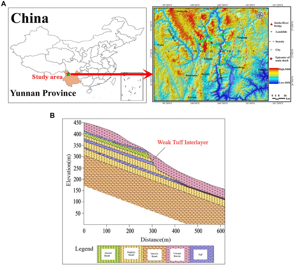
FIGURE 1. (A) Location of the landslide, Yunnan Province, China, (B) The longitudinal geological profile of the landslide.

Numerical Model

Principle of CDEM

Continuum-Discontinuum Element Method (CDEM) is a new type of numerical method developed on the basis of the rigid block discrete element method. In the numerical simulation, the computational domain is generally discretized into units for calculation. For these elements, they can be continuous(corresponding to the finite element method), discontinuous(corresponding to the discrete element method), and partially continuous(corresponding to the CDEM method), as shown in Figure 2A (springs include normal and tangential springs). The finite element method is used to solve completely continuous problems, while the discrete element method is suitable for fully discontinuous problems, generally. CDEM combines the advantages of continuous calculation and discrete calculation, that is, finite element calculation in the block and discrete element calculation at the boundary to realize the progressive failure process of the rock mass. As shown in Figure 2B, the computational domain in CDEM is composed of blocks and virtual interfaces. The blocks, composed of finite element, is used to calculate the elastic, plastic and other continuous properties of rocks. The virtual interfaces refer to the common boundaries between blocks, which are composed of normal penalty springs and tangential penalty springs, and their cracking and sliding can characterize the discontinuous features of rocks.

FIGURE 2

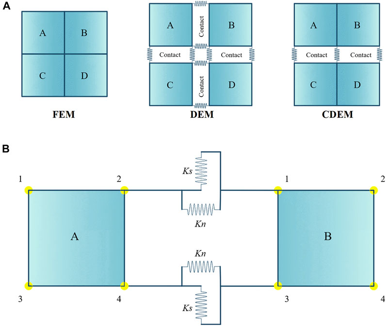
FIGURE 2. (A) Comparison of computational domains FEM, DEM, and CDEM; (B) 2D contacts in CDEM contacts A2 - B1 and A4 - B3.

In the CDEM calculation, the constitutive of the tensile-shear composite interface based on the fracture energy is used to calculate the fracture of the rock virtual interface. Use the following equations to calculate the contact forces at the next time step on the interface:

$F_{\text{n}}\left(t_1\right)=F_{\text{n}}\left(t_0\right)-k_n{A}_c\Delta u_{\text{n}}(1)$

$F_{\text{s}}\left(t_1\right)=F_{\text{s}}\left(t_0\right)-k_{\text{s}}{A}_{\text{c}}\Delta u_{\text{s}}(2)$

where F_n and F_s are contact forces of the normal and tangential penalty spring, respectively; k_n and k_s are contact stiffness of the normal and tangential penalty spring (Pa/m), respectively; A_c is the contact area; Δu_s and Δu_n are the relative displacement increment in tangential and normal directions, respectively.

The tensile failure criterion is expressed as follows:

$\mathrm{I}\mathrm{f}-F_{\text{n}}\left(t_1\right)\ge {\sigma }_{\text{t}}\left(t_0\right)A_c(3)$

$\text{then}{F}_{\text{n}}\left(t_1\right)=-{\sigma }_{\text{t}}\left(t_0\right)A_{\text{c}}(4)$

${\sigma }_t\left(t_1\right)=-{\left({\sigma }_{t0}\right)}^2\Delta u_{\text{n}}/\left(2G_{\text{ft}}\right)+c_0(5)$

where σ_t0, σ_t (t₀) and σ_t (t₁) are the tensile strengths at the initial moment, this moment and the next moment, respectively; G_ft is the tensile fracture energy (Pa·m).

The shear failure criterion is expressed as follows:

$\text{If}{F}_{\text{s}}\left(t_1\right)\ge F_{\text{n}}\left(t_1\right)\tan \mathit{\Phi }+c\left(t_0\right)A_{\text{c}}(6)$

$\text{then}{F}_{\text{s}}\left(t_1\right)=F_{\text{n}}\left(t_1\right)\tan \mathit{\Phi }+c\left(t_0\right)Ac(7)$

$c\left(t_1\right)=-c_0^2\Delta u_{\text{s}}/\left(2G_{\text{fs}}\right)+c_0(8)$

where c₀, c (t₀), and c (t₁) are the cohesion at the initial moment, this moment and the next moment, respectively; Φ is the internal friction angle of the virtual interface; G_fs is the shear fracture energy (Pa·m).

According to the above description, the tensile-shear constitutive curve considering the fracture energy is drawn as shown in Figure 3.

FIGURE 3

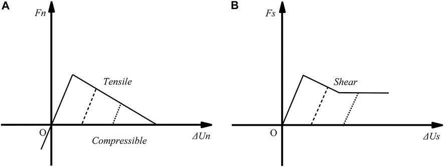
FIGURE 3. Relationship between the bonding stress and opening sliding displacement (A) under compression and tension conditions; (B) under shear and sliding conditions.

CDEM is a dynamic explicit solution algorithm based on breakable elements under the Lagrangian system, and is solved by the explicit Euler forward difference method based on the incremental method. The solution is divided into three steps: (1) calculate the deformation force and damping force of the blocks by cycling each finite element; (2) cycle each contact surface to calculate the connection force and damping force of the contact surface; (3) cycle all nodes to calculate the joint external force, acceleration, velocity, and displacement. The specific calculation process is shown in Figure 4.

FIGURE 4

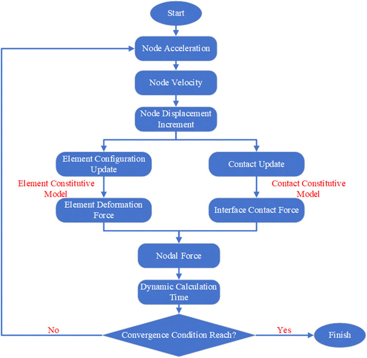
FIGURE 4. Flowchart of the iteration process in CDEM.

Numerical Modeling

In the numerical simulation, the effects of different weak interlayer dip angles and amplitudes are considered. Three groups of weak interlayer dip angles, i.e. 15°, 30°, and 45°, are analyzed; and four groups of input amplitudes, i.e. 0.3, 0.5, 0.8, and 1.0 g, are studied. Table 1 shows the specific calculation scheme.

TABLE 1

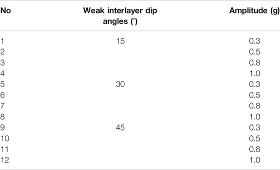
TABLE 1. Calculation conditions in numerical simulation.

Figure 5 shows the slope geometry, monitoring point layout, and grid division in the numerical simulation. All of the slope height is 450 m. For dynamic calculations, to eliminate the influence of artificial boundaries, the bottom of the model adopts a viscous boundary, and the normal displacement of the bottom is fixed. Use free field boundaries on the left and right sides of the model to absorb false vibrations. Apply sine waves of different amplitudes at the bottom of the model, and Figure 6 shows the amplitude time history curve. In CDEM, to impose a dynamic load of stress-time history on the viscous boundary, it is necessary to integrate the acceleration time history into a velocity-time history and then convert it into a stress-time history. The conversion expression is as follows:

${\sigma }_{\text{n}}=2\left(\rho \cdot C_{\text{p}}\right)v_{\text{n}}(9)$

${\sigma }_{\text{s}}=2\left(\rho \cdot C_{\text{s}}\right)v_{\text{s}}(10)$

where C_p is P-wave velocity and C_s is S-wave velocity; v_n and v_s represent normal and tangential velocity, respectively. In the numerical calculation, 12 monitoring points are set up on the slope surface and in the slope, to monitor the acceleration of the slope. The test results can be used to study the acceleration change characteristics and amplification effects, so as to analyze the dynamic response.

FIGURE 5

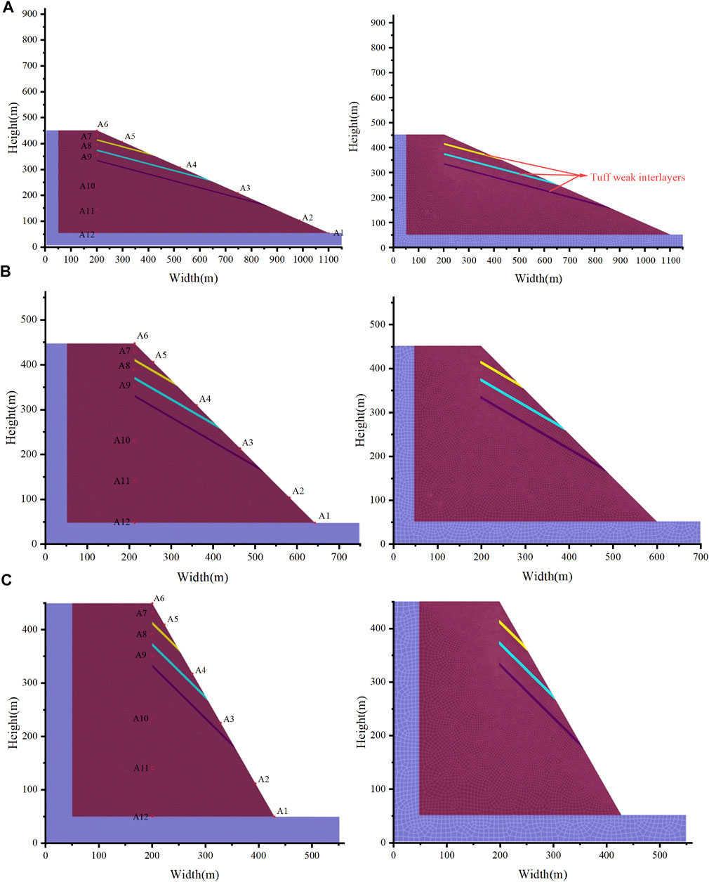
FIGURE 5. Model geometry, monitoring point layout and grid division (A) weak interlayers dip is 15°, (B) weak interlayers dip is 30°, (C) weak interlayers dip is 45°.

FIGURE 6

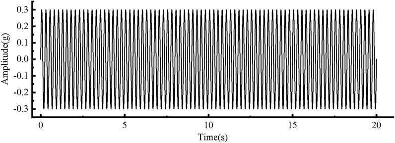
FIGURE 6. Harmonic waves used as input base excitations.

In CDEM, the selection of material parameters is important content. The material parameters in CDEM include bulk parameters that characterize continuity and numerical spring parameters that characterize discontinuity. In this study, the block parameters are obtained based on experiments. Table 2 shows the rock block parameters used in numerical simulation, and Table 3 gives the numerical springs parameters. The micro-parameters parameters used in the numerical modelling can be determined by the method in the published papers (Li et al., 2006; Feng et al., 2014; Li et al., 2015). Among them, use the following equation to calculate the normal stiffness and tangential stiffness:

$K=A{E}_{\text{r}}/\left(2T_0\right)(11)$

where A is the contact area, E_r denotes the young’s modulus, T₀ denotes the thickness of the structural layer, and its size is usually 1% of the size of the block.

TABLE 2

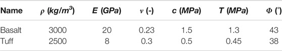
TABLE 2. Parameters of block elements in the numerical calculation.

TABLE 3

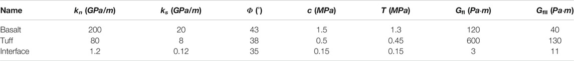
TABLE 3. Parameters of the contact elements in the numerical calculation.

The expressions of tensile fracture energy and shear fracture energy are as follows:

$G_{\text{ft}}=K_{\text{IC}}^2/E(12)$

$G_{\text{fs}}=\left(1-v^2\right)K_{\mathrm{I}\mathrm{I}C}^2/E(13)$

where K_ⅠC and K_ⅡC are tensile and shear fracture toughness.

To ensure the correctness of the numerical calculation results, the validity of the parameters used is verified by a uniaxial compression test. Figure 7 shows the geometric model and results of the uniaxial compression test.

FIGURE 7

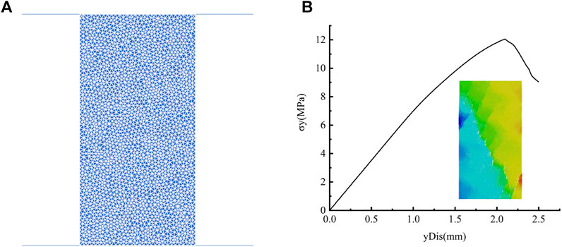
FIGURE 7. Numerical verification for uniaxial compression testing in CDEM (A) model geometry and (B) failure curve and failure state.

Analysis of Simulation Results

The failure modes of landslides are studied by analyzing the failure process, waveform characteristics, amplification effect, and crack ratio in this section.

Analysis of Landslide Failure Process

The dynamics failure process of the landslide is shown in Figure 8. Figure 8A; Figure 8B show the displacement distributions ((A) 0.5 g amplitude; (B) 1.0 g amplitude) of the failure process of the slope with 15°-dip-angle weak interlayers. Figure 8A; Figure 8B shows that the slope with 15° inclination angle weak interlayers is only partially damaged under the action of earthquakes with different amplitudes, but does not reach the overall instability slip. This kind of slope has similar failure disciplines under the effect of earthquakes of different amplitudes: (1) The contact surface of weak interlayers was damaged and broken (t = 0.1–4.0 s); (2) Vertical tension cracking occurred on the back edge of the slope. The rock mass on the slope surface, meanwhile, was damaged to generate micro-cracks since the amplification effect of the seismic wave (t = 8.0-12.0 s); (3) The tensile crack at the trailing edge of the slope widened and continued to spread downward, but it never penetrated the fracture surface produced by the weak interlayers. This is the reason why the overall slip failure did not occur under these conditions. In addition, for the damaged weak interlayers that have a downward sliding trend, the broken rock blocks were driven to slide downward, forming a small number of falling rocks (t = 16.0-19.8 s). It is noted that when the amplitude is small (0.3–0.8 g), the slope failure mainly occurs above the third weak interlayer, and the weak interlayers play a principal role in slope failure. As for large amplitude (1.0 g), the slope toe was damaged (Figure 8B), indicating that the effect of strong earthquakes is greater than that of weak interlayers. The toe of the slope was squeezed out under the action of strong earthquakes due to stress concentration.

FIGURE 8

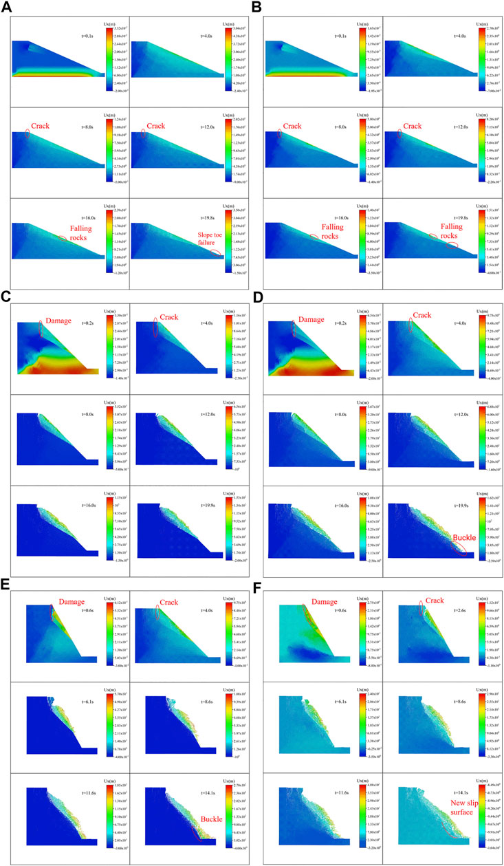
FIGURE 8. The failure process of the slope (A) 0.5 g-15°, (B) 1.0 g-15°, (C) 0.5 g-30°, (D) 1.0 g-30°, (E) 0.5 g-45°, (F) 1.0 g-45°.

Figure 8C; Figure 8D show the displacement distributions ((C) 0.5 g amplitude; (D) 1.0 g amplitude) of the failure process of the slope with 30° dip angle weak interlayers. From Figure 8C; Figure 8D, the slopes with 30°-dip-angle weak interlayers are completely destroyed under the action of earthquakes, and the final slip surface is mainly controlled by the third weak interlayer. Under different amplitudes, the failure process of slopes shows similar disciplines: (1) Damage and cracking occurred on the contact surfaces of the weak interlayers (t = 0.2 s); (2) Vertical tension cracks occurred on the back edge of the slope. At the angle between the fractured surfaces and the weak interlayers, the rock masses were destroyed due to stress concentration, and a small amount of rock fell (t = 4.0 s); (3) The tensile cracks on the back edge widened and expanded downwards, intersecting with the first weak intercalation, and the rock masses above the first weak interlayer slipped downward (t = 8.0 s); (4) The trailing edge cracks continued to propagate downward, and successively penetrated the second and third weak interlayers (t = 12.0 s and t = 16.0 s), causing the rock masses above the third weak interlayer to collapse. Finally, the overall collapse was formed (t = 19.9 s). It is worth mentioning that when the amplitude is small (0.3 and 0.5 g), no damage occurs at the slope toe, and the third weak interlayer is the control sliding surface, where in the case of large amplitude (0.8 and 1.0 g), the slope toe is damaged. The rock mass below the third weak interlayer appears buckling failure, but no new slip surface is formed.

Figure 8E; Figure 8F show the displacement distributions ((E) 0.5 g amplitude; (F) 1.0 g amplitude) of the failure process of the slope with 45°-dip-angle weak interlayers. From Figure 8E; Figure 8F, the slope with weak interlayers with an inclination angle of 45° has overall instability and destructiveness. The failure process is expressed: (1) The contact surfaces of the weak interlayers were damaged and cracked (t = 0.4 s); (2) Vertical tension cracks occurred on the back edge of the slope. The rock mass above the third weak interlayer, meanwhile, slipped as a whole (t = 2.6 s); (3) The cracks on the trailing edge were widened and extended downwards to penetrate the weak interlayers. The slope top blocks collapsed (t = 6.1–8.6 s); (4) Under the control of the weak interlayers, the slope fell as a whole. There are different final failure modes under different amplitudes. Under the condition of an amplitude of 0.3 g, the slope toe does not damage, and the final slip surface is controlled by the third weak interlayer; In the case of an amplitude of 0.5 g, the slope toe undergoes extrusion failure and the rock masses below the third weak interlayer buckle, but no new slip surface is formed; The rock masses below the third weak interlayer are destroyed as a whole and penetrates through the upper slip surface to form a new integral slip surface when the amplitude is above 0.8 g.

Analysis of Waveform Characteristics

In the numerical simulation, 12 monitoring points are arranged (Figure 5). Obtain the acceleration time-history curve from the acceleration data of the monitoring points. Figure 9 shows the acceleration time-history curves with weak interlayers inclination of 15° under the input wave of amplitude 0.5 g. According to Figure 9, the waveform fluctuates uniformly throughout the entire process without obvious discrete points at the two monitoring blocks A1 and A2, indicating that there is no damage at the two places, that is, no damage occurs below the third weak interlayer. The waveforms of A3-A6 produced different degrees of fluctuation dispersion phenomenon at different moments. After the first fluctuation dispersion, there will still be multiple wave dispersion phenomena in a relatively short period, and then enter the relatively uniform fluctuation phase. The reason for this phenomenon is that: when discrete fluctuations appear for the first time, it indicates that the connection of the monitoring block is broken and microcracks are generated, which leads to a sharp change in acceleration. However, the constraints between the monitoring block and the adjacent blocks have not been completely lifted, and the collision between the blocks makes the acceleration change drastically. After the connection between the monitoring block and the adjacent blocks is completely broken, the monitoring block slides out or flies out, and the acceleration fluctuates uniformly, that is, the waveform is uniformly distributed. As shown in Figure 9, A7-A12 monitoring blocks all have discrete waveform fluctuations at different times, indicating that damage occurs inside the slope at different times. After damage, the waveform fluctuates uniformly or discretely again. The reason is that: the A7-A12 monitoring blocks are located inside the slope. After the damage occurs, the damaged monitoring block cannot slide due to the constraints of the surrounding blocks, so the waveform is evenly distributed. However, the damaged block may suffer connection damage again, causing discrete fluctuations in the waveform again.

FIGURE 9

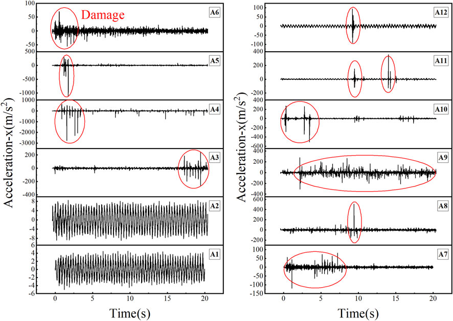
FIGURE 9. Acceleration time-history curve of calculation condition with weak interlayers of 15° and amplification of 0.5 g.

According to the above analysis, for the calculation condition with weak interlayers inclination of 15° and an amplitude of 0.5 g, no damage occurs at A1-A2, that is, no damage occurs below the third weak interlayer. The different degrees of damage occurred at A3-A6, indicating that under the influence of the weak interlayers, the upper part of the slope appears to be damaged and slipped, and the weak interlayers are the key cause of slope instability. Different degrees of damage occurred in A7-A12, indicating that the earthquake will cause internal damage to the slope and produce more micro-cracks. These micro-cracks are unstable factors that threaten the safety of the slope. More, the sequence of a slope failure can be determined by using the time when the discrete waveform appears. The time sequence of slope failure is A6, A5, A4, A3 at the slope surface, indicating that with the effort of the weak interlayers, the upper weak interlayer is destroyed first, driving the rock above the upper weak interlayer to slip, and then the lower rock layer is successively destroyed. In the interior of the slope, A7-A10 are destroyed first, A11 and A12 are destroyed in sequence, and the order of destruction is from the top to the bottom of the slope.

Other calculation conditions show similar disciplines. It is worth mentioning that under these two conditions, the slope toe (A1) and the lower part of the weak interlayer (A2) were damaged, and the third weak interlayer (A3) was the first to fail and slip. This is because when the inclination angle is relatively large, seismic action is no longer the only dominant factor in slope failure. The combined effort of the earthquake and geological structure makes the third weak interlayer break out first, and then drive the upper rock formation to slide.

Dynamic Amplification Effect Analysis

The amplification effect of the slopes takes into account the influence of the weak interlayers dip and the amplitude of the seismic load. Here use the peak ground displacement (PGD) to describe the dynamic response of the slopes. Introduce the PGD amplification coefficient, i.e. the ratio of the PGD of any monitoring point to the PGD at the slope toe (A1), and the relative height (h/H), i.e. the ratio of the height of any monitoring point to the height of the slope. Figure 10 shows the PGD amplification coefficient under various calculation conditions. As the height increases, the PGD amplification coefficient increases first and then decreases overall.

FIGURE 10

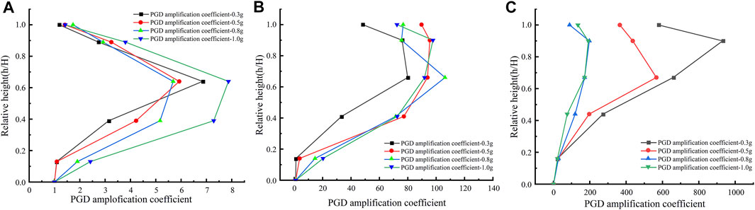
FIGURE 10. Variation of PGD amplification coefficient with relative height (A) weak interlayers dip is 15°, (B) weak interlayers dip is 30°, (C) weak interlayers dip is 45°.

From Figure 10A, for a slope with weak interlayers inclination of 15°, the PGD amplification coefficient increases sharply in the middle of the slope (A3, A4, and A5), indicating that this is the main area of slope failure, that is, the slope failure is mainly controlled by the weak interlayers under this calculation condition. Note that the slope toe is not damaged when the amplitude is below 0.5 g, and the PGD amplification coefficient of the slope lower part (A2) is very small; and when the amplitude is above 0.8 g, the slope toe is damaged. The slope lower part (A2) produces a large displacement, and its PGD amplification coefficient also increases. Figure 10B shows the PGD amplification coefficient of slopes with weak interlayers inclination of 30°. Similar to the inclination angle of 15°, the amplification coefficient of PGD in the middle and upper part of the slope increases sharply. The slope toe is not damaged when the amplitude is 0.3 g, and the PGD amplification coefficient is small, and when the amplitude is greater than 0.5 g, the PGD amplification coefficient of the lower slope is increased due to the damage of the slope toe. The slope with an inclination angle of 30°, different from the slope with an inclination angle of 15°, has an overall slippage above the weak interlayers, so the overall PGD amplification coefficient is very large. And the slope top (A6) has a large slippage, where the PGD amplification coefficient is large. Figure 10C shows the PGD amplification coefficient of the slope with weak interlayers inclination angle of 45°. Under these conditions, the slope toe is damaged. Because the slope toe does not have a large slip as the amplitude of the slope is below 0.5 g, its PGD is small, making the middle and upper PGD amplification coefficient very large. When the amplitude is greater than 0.8g, the slope toe slides out, and its PGD is larger, making the overall PGD amplification factor smaller. From Figure 10C, the slope damage is mainly concentrated in the middle and upper part for the effect of the weak interlayers.

Comparing the above results, the slope damage, when the inclination angle is small (15°), mainly occurs in the middle and upper part, especially in the middle part, indicating that the failure of this type of slopes is mainly controlled by the weak interlayers, and the third weak interlayer has the most obvious effect. When the inclination angle is large (30° and 45°), the slopes are damaged by sliding as a whole, even the slope toe fails, too. In terms of the damage degree, the middle part of the slope is the most serious, followed by the top and toe of the slope, indicating that the weak interlayers still play an important part in the damage to this type of slope. However, with the increase of inclination angle and amplitude, the slope toe is squeezed out under the dynamic loads, and the failure control surface of the slopes change from the weak interlayers to the combination of weak interlayers and slope toe.

Equivalent Crack Ratio Analysis

The concept of spring equivalent crack ratio is introduced to characterize the slope failure degree. The definition formula of spring equivalent crack ratio is:

$R=S_1/S_0(14)$

where R is the spring equivalent crack ratio, S₁ is the cumulative value of the product of the spring damage factor and the area, and S₀ is the total contact area of the blocks. The equivalent crack ratio under different calculation conditions is shown in Figure 11. As the loading time increases, the equivalent crack ratio first increases sharply and then gradually stabilizes. According to Figure 11, the development of the equivalent crack ratio is divided into three stages: (1) Rapid growth stage (t = 0–4.0 s). At this stage, a large number of micro-cracks are rapidly generated under seismic loads, providing basic conditions for the subsequent failure of the slope. (2) Slowly increasing stage (t = 4.0–12.0 s). The increase in the equivalent crack ratio at this stage is mainly due to the aggregation of the microcracks generated in the previous stage, accompanied by a small number of new micro-cracks, and the growth rate slows down. The aggregation of micro-cracks promotes the failure of slopes. (3) Stable stage (t = 12.0–20.0 s). The equivalent crack ratio increases little at this stage, mainly because the aggregated cracks in the previous stages gradually penetrate and form slip surfaces, which makes the slope instability and failure. After the landslide failure occurs, the accumulated energy is released, and no new microcracks are generated, so the equivalent crack ratio gradually stabilizes.

FIGURE 11

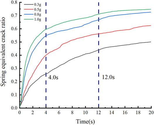
FIGURE 11. Variation of spring equivalent crack ratio with amplifications (weak interlayers dip is 45°).

Figure 12A shows the variation of the final spring equivalent crack ratio with the weak interlayers dip. When the amplitude is small (0.3 and 0.5 g), as the inclination angle increases, the final spring equivalent crack ratio gradually increases, and when the amplitude is large (0.8 and 1.0 g), the final spring equivalent crack ratio changes little as the inclination angle increases. This is because when the amplitude is not large, the weak interlayers have an important influence on slope failure. The seismic load, with the amplitude increasing, becomes the dominant factor for slope failure. As shown in Figure 12B, the final spring equivalent crack ratio has a positive correlation with the amplitude. When the amplitude is greater than 0.8 g, the final spring equivalent crack ratio reaches about 0.7, and the slope reaches failure. It can be seen that earthquakes, especially strong earthquakes, have a devastating effect on slopes.

FIGURE 12

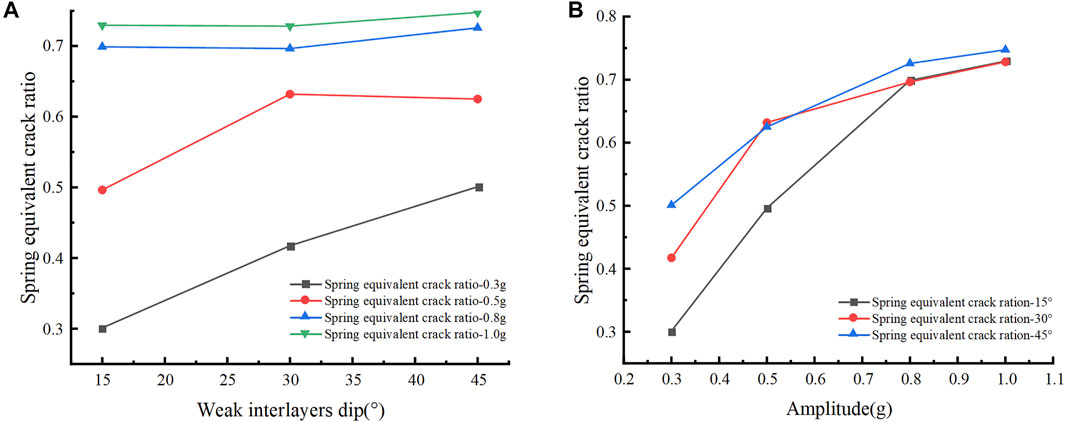
FIGURE 12. Variation of final spring equivalent crack ratio (A) with weak interlayers dips, (B) with amplitudes.

Seismic Failure Mechanism of Landslides

Based on the previous analysis, the numerical results reveal the failure mechanism of landslides with different inclination angles and amplitudes. When the inclination angle of the weak interlayers is 15°, the slope is partially damaged without overall slippage. The main form of slope failure is local rockfall. When the inclination of the weak interlayers is 30°, the slope will slip as a whole. The failure process of the slope can be described as the weak interlayers cracking - tensile cracks appearing on the trailing edge - the tensile cracks widening and expanding downward - the tensile cracks penetrate the weak surfaces and the sliding surface formed, and the landslide is destroyed as a whole. The failure mode can be summarized as “tensile cracking-slip-collapsing”. It is noticed that the slope toe undergoes extrusion failure, but the overall slip surface is not formed as the amplitude reaches 1.0 g. The failure mode of a slope with weak interlayers inclination angle of 45° and an amplitude of less than 0.5 g is akin to that of a slope with an inclination angle of 30°. When the amplitude is equal to or greater than 0.8 g, the failure process is weak interlayer cracking–tensile cracks on the trailing edge–tensile cracks widening and extending downwards - slope toe extrusion–slipping surface penetration, and the overall failure of the landslide. The failure mode can be summarized as “tensile cracking-slip-slope extrusion-collapsing”. Therefore, it can be seen that under different geological conditions, the leading factors of landslide are different, and the combination of weak interlayers and seismic load creates complex landslide failure modes.

Discussion

Research on the stability of weak interbedded rock slopes is a hot issue. Many scholars have carried out research on this issue through field investigation, geological model test, and numerical simulation. Field investigation and geological model test have their own limitations. As computer technology developing rapidly, numerical simulation has become a good choice for studying the progressive failure process of landslides with complex geological structures.

The traditional numerical simulation methods, including the finite element method (FEM) and discrete element method (DEM), are widely used in calculating slope stability. The finite element method usually cannot simulate the large deformation and failure of rock slopes, especially the dynamic slip process accompanied by the seismic load of complex geological structures. The discrete element method can simulate the large deformation and the entire failure process of the slope, but due to its complex contact detection and low calculation efficiency, large-scale calculations are time-consuming. The CDEM method combines the advantages of the two traditional numerical methods and can realize the transformation of rock materials from continuum to discontinuum. Studies have shown that it is an effective method for simulating geological disasters such as landslides.

The CDEM simulation results show that different failure modes occur under different weak interlayers and seismic load combinations: local rockfall occurs in a gentle slope, “tensile cracking-slip-collapsing” failure occurs in mid-dip slope, and “tensile cracking-slip-slope extrusion-collapsing” failure occurs in a steep slope. Besides, the waveform characteristics, PGD amplification coefficient, and spring equivalent crack ratio have consistent correspondence with the failure process of landslides. The discrete fluctuations of the acceleration waveform indicate the cracking failure of the rock blocks, and the characteristics of the waveform reveal the failure location and failure time of landslides. The sudden change of the PGD amplification coefficient reflects the damaged location and damage degree of landslides. It is worth mentioning that the slope failure process can be divided into three stages according to the spring equivalent crack ratio: equivalent crack ration rapid increase stage, equivalent crack ration slow increase stage, and equivalent crack ration stable stage. This reveals the failure mechanism of landslides: under the action of the earthquake, a large number of micro-cracks are rapidly generated first, and then the micro-cracks are expanded and aggregated, and finally the cracks penetrate to form a slip surface and cause a landslide. The failure process of landslides can be divided and the failure mechanism of landslides can be explained based on the analysis of the equivalent crack ratio, which provides a reference for the criterion of landslides.

However, CDEM numerical simulation in this study has its own limitations. The real geological structure is in a three-dimensional state, and it is difficult for two-dimensional numerical simulation to accurately reflect the three-dimensional motion characteristics of landslides. Also, the variation of parameters that is not considered in this paper will be an important factor for the failure modes. We will try to carry out three-dimensional related research and parameters discussion in future work. In addition, some laboratory experiments contain important information for understanding the mechanism of earthquake-induced landslides, which are of high value for simulation and verification(Burridge and Knopoff, 1967; Parteli et al., 2005). We will consider these experimental information in the future research. Although the simulation has limitations, a reference to reveal the failure process and failure mechanism of rock slopes under the combined action of weak interlayers and earthquakes is provided. In addition, CDEM method is not only suitable for earthquake-induced landslides simulation, but also applied to model a broader range of landslide types, for example, cumulative perturbations due to soil instability processes(Feng et al., 2014; Yongbo et al., 2016). CDEM method provides new ideas for studying geological disasters such as landslides.

Conclusions

The CDEM method is used to numerically simulate the failure modes and dynamic response of weak interbedded rock slopes under earthquakes. Some conclusions can be drawn as follows:

1. The characteristics of acceleration waveform and PGD amplification coefficient have strong consistency with the landslide failure process. The discrete fluctuation of the waveform reflects the damage location and time of the landslide. The sharp change of the PGD amplification coefficient reveals the landslide damage location and damage degree.

2. The concept of spring equivalent crack ratio is introduced, and the landslide development process can be divided into three stages by using the change of spring equivalent crack ratio over time: rapid generation of a large number of microcracks, expansion, and aggregation of microcracks, and penetration of micro-cracks and the formation of slip surfaces.

3. The combination of weak interlayers and seismic load causes multiple failure modes of the landslide. For the gentle slope (15°), local damage occurs on the slope, and the main form of damage is rockfall. For a mid-dip slope (30°), the slope has an overall failure, and the failure mode is “tensile cracking-slip-collapsing”. For the steep slope (45°), “tensile cracking-slip-collapsing” failure occurs when the amplitude is small, and “tensile cracking-slip-slope extrusion-collapsing” failure occurs when the amplitude is large.

Data Availability Statement

Publicly available datasets were analyzed in this study. This data can be found here: http://www.civil.tsinghua.edu.cn/he/essay/340/956.html.

Author Contributions

XL designed the research; CW performed the research; DS, EW, and JZ wrote sections of the manuscript; and CW and XL organized and wrote the paper. All authors read and approved the manuscript.

Funding

This work was supported by the National Key R&D Program of China (Grant No. 2018YFC1504902), the National Natural Science Foundation of China (Grant No. 52079068), and the State Key Laboratory of Hydroscience and Hydraulic Engineering (Grant No. 2021-KY-04).

Conflict of Interest

The authors declare that the research was conducted in the absence of any commercial or financial relationships that could be construed as a potential conflict of interest.

Publisher’s Note

All claims expressed in this article are solely those of the authors and do not necessarily represent those of their affiliated organizations, or those of the publisher, the editors and the reviewers. Any product that may be evaluated in this article, or claim that may be made by its manufacturer, is not guaranteed or endorsed by the publisher.

Acknowledgments

Special thanks to Gdem Technology, Beijing, Co., Ltd. for its technical support.

References

Bao, Y., Han, X., Chen, J., Zhang, W., Zhan, J., Sun, X., et al. (2019). Numerical Assessment of Failure Potential of a Large Mine Waste Dump in Panzhihua City, China. Eng. Geology. 253, 171–183. doi:10.1016/j.enggeo.2019.03.002

CrossRef Full Text | Google Scholar

Burridge, R., and Knopoff, L. (1967). Model and Theoretical Seismicity. Bull. Seismological Soc. America 57, 341–371. doi:10.1785/bssa0570030341

CrossRef Full Text | Google Scholar

Chen, Z., and Song, D. (2021). Numerical Investigation of the Recent Chenhecun Landslide (Gansu, China) Using the Discrete Element Method. Nat. Hazards 105, 717–733. doi:10.1007/s11069-020-04333-w

CrossRef Full Text | Google Scholar

Cui, S., Yang, Q., Pei, X., Huang, R., Guo, B., and Zhang, W. (2020). Geological and Morphological Study of the Daguangbao Landslide Triggered by the Ms. 8.0 Wenchuan Earthquake, China. Geomorphology 370, 107394. doi:10.1016/j.geomorph.2020.107394

CrossRef Full Text | Google Scholar

Dai, F. C., Xu, C., Yao, X., Xu, L., Tu, X. B., and Gong, Q. M. (2011). Spatial Distribution of Landslides Triggered by the 2008 Ms 8.0 Wenchuan Earthquake, China. J. Asian Earth Sci. 40, 883–895. doi:10.1016/j.jseaes.2010.04.010

CrossRef Full Text | Google Scholar

Delgado, J., Rosa, J., Peláez, J. A., Rodríguez-Peces, M. J., Garrido, J., and Tsigé, M. (2020). Newmark Displacement Data for Low to Moderate Magnitude Events in the Betic Cordillera. Data in Brief 32, 106097. doi:10.1016/j.dib.2020.106097

PubMed Abstract | CrossRef Full Text | Google Scholar

Deng, Z., Liu, X., Liu, Y., Liu, S., Han, Y., Liu, J., et al. (2020). Model Test and Numerical Simulation on the Dynamic Stability of the Bedding Rock Slope under Frequent Microseisms. Earthq. Eng. Eng. Vib. 19, 919–935. doi:10.1007/s11803-020-0604-8

CrossRef Full Text | Google Scholar

Do, T. N., and Wu, J.-H. (2020). Simulating a Mining-Triggered Rock Avalanche Using DDA: A Case Study in Nattai North, Australia. Eng. Geology. 264, 105386. doi:10.1016/j.enggeo.2019.105386

CrossRef Full Text | Google Scholar

Donati, D., Stead, D., Stewart, T. W., and Marsh, J. (2020). Numerical Modelling of Slope Damage in Large, Slowly Moving Rockslides: Insights from the Downie Slide, British Columbia, Canada. Eng. Geology. 273, 105693. doi:10.1016/j.enggeo.2020.105693

CrossRef Full Text | Google Scholar

Feng, C., Li, S., Liu, X., and Zhang, Y. (2014). A Semi-spring and Semi-edge Combined Contact Model in CDEM and its Application to Analysis of Jiweishan Landslide. J. Rock Mech. Geotechnical Eng. 6, 26–35. doi:10.1016/j.jrmge.2013.12.001

CrossRef Full Text | Google Scholar

Huang, M., Fan, X., and Wang, H. (2017). Three-dimensional Upper Bound Stability Analysis of Slopes with Weak Interlayer Based on Rotational-Translational Mechanisms. Eng. Geology. 223, 82–91. doi:10.1016/j.enggeo.2017.04.017

CrossRef Full Text | Google Scholar

Huang, M., Wang, H., Sheng, D., and Liu, Y. (2013). Rotational-translational Mechanism for the Upper Bound Stability Analysis of Slopes with Weak Interlayer. Comput. Geotechnics 53, 133–141. doi:10.1016/j.compgeo.2013.05.007

CrossRef Full Text | Google Scholar

Huang, R., Xiao, H., Ju, N., and Zhao, J. (2007). Deformation Mechanism and Stability of a Rocky Slope. J. China Univ. Geosciences 18, 77–84. doi:10.1016/s1002-0705(07)60021-1

CrossRef Full Text | Google Scholar

Kawamura, S., Kawajiri, S., Hirose, W., and Watanabe, T. (2019). Slope Failures/landslides over a Wide Area in the 2018 Hokkaido Eastern Iburi Earthquake. Soils and Foundations 59, 2376–2395. doi:10.1016/j.sandf.2019.08.009

CrossRef Full Text | Google Scholar

Li, C., Wu, J., Tang, H., Hu, X., Liu, X., Wang, C., et al. (2016). Model Testing of the Response of Stabilizing Piles in Landslides with Upper Hard and Lower Weak Bedrock. Eng. Geology. 204, 65–76. doi:10.1016/j.enggeo.2016.02.002

CrossRef Full Text | Google Scholar

Li, S. H., Wang, J. G., Liu, B. S., and Dong, D. P. (2006). Analysis of Critical Excavation Depth for a Jointed Rock Slope Using a Face-To-Face Discrete Element Method. Rock Mech. Rock Engng. 40, 331–348. doi:10.1007/s00603-006-0084-9

CrossRef Full Text | Google Scholar

Li, Z., Wang, J. a., Li, L., Wang, L., and Liang, R. Y. (2015). A Case Study Integrating Numerical Simulation and GB-InSAR Monitoring to Analyze Flexural Toppling of an Anti-dip Slope in Fushun Open Pit. Eng. Geology. 197, 20–32. doi:10.1016/j.enggeo.2015.08.012

CrossRef Full Text | Google Scholar

Lin, C.-H., Li, H.-H., and Weng, M.-C. (2018). Discrete Element Simulation of the Dynamic Response of a Dip Slope under Shaking Table Tests. Eng. Geology. 243, 168–180. doi:10.1016/j.enggeo.2018.07.005

CrossRef Full Text | Google Scholar

Lin, P., Liu, X., Hu, S., and Li, P. (2016). Large Deformation Analysis of a High Steep Slope Relating to the Laxiwa Reservoir, China. Rock Mech. Rock Eng. 49, 2253–2276. doi:10.1007/s00603-016-0925-0

CrossRef Full Text | Google Scholar

Liu, C., Liu, X., Peng, X., Wang, E., and Wang, S. (2019). Application of 3D-DDA Integrated with Unmanned Aerial Vehicle-Laser Scanner (UAV-LS) Photogrammetry for Stability Analysis of a Blocky Rock Mass Slope. Landslides 16, 1645–1661. doi:10.1007/s10346-019-01196-6

CrossRef Full Text | Google Scholar

Liu, X., Han, G., Wang, E., Wang, S., and Nawnit, K. (2018). Multiscale Hierarchical Analysis of Rock Mass and Prediction of its Mechanical and Hydraulic Properties. J. Rock Mech. Geotechnical Eng. 10, 694–702. doi:10.1016/j.jrmge.2018.04.003

CrossRef Full Text | Google Scholar

Luo, J., Pei, X., Evans, S. G., and Huang, R. (2019). Mechanics of the Earthquake-Induced Hongshiyan Landslide in the 2014 Mw 6.2 Ludian Earthquake, Yunnan, China. Eng. Geology. 251, 197–213. doi:10.1016/j.enggeo.2018.11.011

CrossRef Full Text | Google Scholar

Marcato, G., Mantovani, M., Pasuto, A., Zabuski, L., and Borgatti, L. (2012). Monitoring, Numerical Modelling and hazard Mitigation of the Moscardo Landslide (Eastern Italian Alps). Eng. Geology. 128, 95–107. doi:10.1016/j.enggeo.2011.09.014

CrossRef Full Text | Google Scholar

Martino, S., Lenti, L., and Bourdeau, C. (2018). Composite Mechanism of the Büyükçekmece (Turkey) Landslide as Conditioning Factor for Earthquake-Induced Mobility. Geomorphology 308, 64–77. doi:10.1016/j.geomorph.2018.01.028

CrossRef Full Text | Google Scholar

Montgomery, J., Candia, G., Lemnitzer, A., and Martinez, A. (2020). The September 19, 2017 Mw 7.1 Puebla-Mexico City Earthquake: Observed rockfall and Landslide Activity. Soil Dyn. Earthquake Eng. 130, 105972. doi:10.1016/j.soildyn.2019.105972

CrossRef Full Text | Google Scholar

Newmark, N. M. (1965). Effects of Earthquakes on Dams and Embankments. Géotechnique 15, 139–160. doi:10.1680/geot.1965.15.2.139

CrossRef Full Text | Google Scholar

Parteli, E. J., Gomes, M. A., and Brito, V. P. (2005). Nontrivial Temporal Scaling in a Galilean Stick-Slip Dynamics. Phys. Rev. E Stat. Nonlin Soft Matter Phys. 71, 036137. doi:10.1103/PhysRevE.71.036137

PubMed Abstract | CrossRef Full Text | Google Scholar

Sangirardi, M., Amorosi, A., and De Felice, G. (2020). A Coupled Structural and Geotechnical Assessment of the Effects of a Landslide on an Ancient Monastery in Central Italy. Eng. Structures 225, 111249. doi:10.1016/j.engstruct.2020.111249

CrossRef Full Text | Google Scholar

Seisdedos, J., Ferrer, M., and González de Vallejo, L. I. (2012). Geological and Geomechanical Models of the Pre-landslide Volcanic Edifice of Güímar and La Orotava Mega-Landslides (Tenerife). J. Volcanology Geothermal Res. 239-240, 92–110. doi:10.1016/j.jvolgeores.2012.06.013

CrossRef Full Text | Google Scholar

Song, D., Chen, Z., Chao, H., Ke, Y., and Nie, W. (2020). Numerical Study on Seismic Response of a Rock Slope with Discontinuities Based on the Time-Frequency Joint Analysis Method. Soil Dyn. Earthquake Eng. 133, 106112. doi:10.1016/j.soildyn.2020.106112

CrossRef Full Text | Google Scholar

Song, D., Liu, X., Huang, J., and Zhang, J. (2021). Energy-based Analysis of Seismic Failure Mechanism of a Rock Slope with Discontinuities Using Hilbert-Huang Transform and Marginal Spectrum in the Time-Frequency Domain. Landslides 18, 105–123. doi:10.1007/s10346-020-01491-7

CrossRef Full Text | Google Scholar

Tang, C.-L., Hu, J.-C., Lin, M.-L., Angelier, J., Lu, C.-Y., Chan, Y.-C., et al. (2009). The Tsaoling Landslide Triggered by the Chi-Chi Earthquake, Taiwan: Insights from a Discrete Element Simulation. Eng. Geology. 106, 1–19. doi:10.1016/j.enggeo.2009.02.011

CrossRef Full Text | Google Scholar

Tang, C., Tang, J., Van Westen, C. J., Han, J., Mavrouli, O., and Tang, C. (2020). Modeling Landslide Failure Surfaces by Polynomial Surface Fitting. Geomorphology 368, 107358. doi:10.1016/j.geomorph.2020.107358

CrossRef Full Text | Google Scholar

Terzaghi, K., and Paige, S. (1950). “Mechanism of Landslides,” in Application of Geology to Engineering Practice (Boulder, USA: Geological Society of America).

Google Scholar

Wasowski, J., Keefer, D. K., and Lee, C.-T. (2011). Toward the Next Generation of Research on Earthquake-Induced Landslides: Current Issues and Future Challenges. Eng. Geology. 122, 1–8. doi:10.1016/j.enggeo.2011.06.001

CrossRef Full Text | Google Scholar

Wu, J.-H., Lin, W.-K., and Hu, H.-T. (2018). Post-failure Simulations of a Large Slope Failure Using 3DEC: The Hsien-Du-Shan Slope. Eng. Geology. 242, 92–107. doi:10.1016/j.enggeo.2018.05.018

CrossRef Full Text | Google Scholar

Xu, J., Tang, X., Wang, Z., Feng, Y., and Bian, K. (2020). Investigating the Softening of Weak Interlayers during Landslides Using Nanoindentation Experiments and Simulations. Eng. Geology. 277, 105801. doi:10.1016/j.enggeo.2020.105801

CrossRef Full Text | Google Scholar

Xu, J., and Yang, X. (2018). Seismic Stability Analysis and Charts of a 3D Rock Slope in Hoek-Brown media. Int. J. Rock Mech. Mining Sci. 112, 64–76. doi:10.1016/j.ijrmms.2018.10.005

CrossRef Full Text | Google Scholar

Xu, W.-J., and Dong, X.-Y. (2021). Simulation and Verification of Landslide Tsunamis Using a 3D SPH-DEM Coupling Method. Comput. Geotechnics 129, 103803. doi:10.1016/j.compgeo.2020.103803

CrossRef Full Text | Google Scholar

Yang, G., Qi, S., Wu, F., and Zhan, Z. (2018). Seismic Amplification of the Anti-dip Rock Slope and Deformation Characteristics: A Large-Scale Shaking Table Test. Soil Dyn. Earthquake Eng. 115, 907–916. doi:10.1016/j.soildyn.2017.09.010

CrossRef Full Text | Google Scholar

Yiğit, A. (2020). Prediction of Amount of Earthquake-Induced Slope Displacement by Using Newmark Method. Eng. Geology. 264, 105385. doi:10.1016/j.enggeo.2019.105385

CrossRef Full Text | Google Scholar

Yongbo, F., Shihai, L., Yang, Z., Zhiyong, F., and Xiaoyu, L. (2016). Lessons Learned from the Landslides in Shengli East Open-Pit Mine and North Open-Pit Mine in Xilinhot City, Inner Mongolia Province, China. Geotech Geol. Eng. 34, 425–435. doi:10.1007/s10706-015-9954-9

CrossRef Full Text | Google Scholar

Yu, Y., Shen, M., Sun, H., and Shang, Y. (2019). Robust Design of Siphon Drainage Method for Stabilizing Rainfall-Induced Landslides. Eng. Geology. 249, 186–197. doi:10.1016/j.enggeo.2019.01.001

CrossRef Full Text | Google Scholar

Yu, Y., Wang, E., Zhong, J., Liu, X., Li, P., Shi, M., et al. (2014). Stability Analysis of Abutment Slopes Based on Long-Term Monitoring and Numerical Simulation. Eng. Geology. 183, 159–169. doi:10.1016/j.enggeo.2014.10.010

CrossRef Full Text | Google Scholar

Zhao, S., Chigira, M., and Wu, X. (2018). Buckling Deformations at the 2017 Xinmo Landslide Site and Nearby Slopes, Maoxian, Sichuan, China. Eng. Geology. 246, 187–197. doi:10.1016/j.enggeo.2018.09.033

CrossRef Full Text | Google Scholar

Zhu, D., Yan, E., Hu, G., and Lin, Y. (2011). Revival Deformation Mechanism of Hefeng Landslide in the Three Gorges Reservoir Based on FLAC3D Software. Proced. Eng. 15, 2847–2851. doi:10.1016/j.proeng.2011.08.536

CrossRef Full Text | Google Scholar