Albedo Parametrizations for the Laohugou Glacier No.12 in the Qilian Mountains—Previous Models and an Alternative Approach

Introduction

Mass loss of glaciers on the Tibetan plateau has been very variable in recent decades, with a strong negative balance in the South-East and near balance in the South-West (Kääb et al., 2012; Brun et al., 2017; Li et al., 2019). This heterogeneous response can be explained with different dominant drivers of accumulation and ablation (Yao et al., 2012). In this rather dry part of high-mountain Asia, glacier melt also constitutes an essential water source for ecosystems and downstream communities (Immerzeel et al., 2020). To assess mass change of an individual glacier while elucidating the drivers of said mass loss a surface energy balance model (SEB) is generally employed, which can be compared against local mass balance measurements. SEBs on clean ice glaciers have been applied on a number of glaciers on the Tibetan Plateau and the wider region including in the Tien Shan (Zhang et al., 2007), the Tanggula mountains (Zhang et al., 1996; Liang et al., 2018), the Qilian mountains (Sakai et al., 2006; Chen et al., 2007; Qing et al., 2018), the central (Zhang et al., 2013; Huintjes et al., 2015a; Huintjes et al., 2015b) and the south-eastern Plateau (Yang et al., 2011) as well as the Himalaya (Yang et al., 2010). The Qilian mountains are located on the north eastern fringe of the plateau, being the water source of many oases downstream. Approximately 2000 glaciers are located in this mountain range, covering an area of 1,057 km² with a total ice volume of 51 km³ (Guo et al., 2015). As it is relatively easily accessible compared to the rest of the plateau, a number of glaciers have been researched in more detail including the Ningchanhe glaciers (Liu et al., 2012), the Bayi glacier (Liu et al., 2020), the Qiyi glacier (Chen et al., 2007) as well as the Laohugou Glacier No. 12 (Sun et al., 2012; Zhang et al., 2012; Sun et al., 2014; Qin et al., 2015; Wang et al., 2018; Liu et al., 2019).

Surface melt has been previously shown to be sensitive to albedo. On the Greenland ice sheet, its sensitivity to albedo is roughly twice than sensitivity to temperature variations (van de Wal, 1996). A number of studies have shown that the SEB of glaciers on the Tibetan Plateau is especially sensitive to changes in albedo, which is not surprising considering that melt in this cold environment is mainly driven by radiation (Fujita et al., 2007; Yang et al., 2011; Sun et al., 2014). Some field observations further indicate that albedo of glacier surfaces has decreased in recent years due to aerosol depositions, resulting in increased melt rates (Wang et al., 2015; Zhang et al., 2017).

Surface albedo is defined as the ratio between reflected and received solar radiation on a predefined surface area and is a result of reflections and refractions at the air ice interface. The proportion reflected is not only determined by properties of the surface itself, but also by the spectral and angular distribution of solar radiation reaching the Earth’s surface. As radiation passes through ice it comes into contact with light-absorbing impurities, and a fraction is absorbed into the surface (Gardner and Sharp, 2010). It can vary greatly in time and space on the glacier, ranging from 0.1 for dirty ice to 0.9 for fresh snow and hence is an important control of surface melt. It is furthermore affected by snow particle size, liquid water content, density, snowpack depth and impurities of the snowpack. Summer snowfall reduces the melting of glaciers and runoff due to the increase in albedo, but snow albedo changes through the melt process and due to impurities (Brock et al., 2000; Jansson et al., 2003). Even relatively small changes in albedo can have significant effects on mass loss on the local and regional scale (Konzelmann and Braithwaite, 1995). On a larger scale albedo also affects the global energy balance and climate and is hence important for regional climate models (Kukla and Kukla, 1974; Sicart et al., 2008; Six et al., 2009).

While many of the studies mentioned above use direct measurements of in- and outgoing radiation, this is often not available in many locations and if only at a point location. To this end net radiation has to be modelled, making use of an albedo model for temporal and spatial variability.

Dunkle and Bevans (1956) proposed a solution based on diffuse radiation and Wiscombe and Warren (1980) developed a method to calculate the spectral albedo of snow at any wavelength. However such approaches remain too complex to be readily applied in any location for a SEB model. Gardner and Sharp (2010) developed a scheme based on the specific surface area of snow/ice, light absorbing carbon, solar zenith angle, cloud optical thickness, and snow depth. Ding et al. (2017) also consider the precipitation type. While all these models have their merits they generally depend on specific insights into the local climate or snow and ice properties. In SEBs generally much simpler approaches are employed. Commonly applied is the model by Oerlemans and Knap (1998) that relies on snow depth and time since last snowfall. Hock and Holmgren (2005) proposed a model that includes information about the current state of the surface boundary layer and needs as input air temperature, solid precipitation and days since last snowfall. It also relies on the albedo of the preceding timestep and hence is very sensitive to the initial choice of this value. Brock et al. (2000) test a number of parametrisations and find that information of the physical properties of snow should be included for an accurate derivation of albedo. They hence propose a model with different parameters at different snow depths that relies on air temperature and the time since the last snow fall, in this way reproducing the decay of the snowpack.

In this study we employ a coupled energy and mass balance model (COSIMA) that has been developed on the Tibetan Plateau (Huintjes et al., 2015a; Huintjes et al., 2015b) and test its performance at a glacier site in the Qilian mountains. A previous study on the glacier has already tested the suitability of the common bulk aerodynamic model to reproduce the turbulent fluxes, by comparing it against direct measurements of turbulence (Sun et al., 2014). They show that the models generally work well but that turbulent fluxes are considerably less relevant for melt than radiative fluxes. They also show that the SEB is especially sensitive to the change in albedo.

We have collected 6 years of surface flux and mass balance data on Laohugou No. 12 Glacier in the Qilian mountains, which allows us to investigate the importance of albedo for mass balance estimates as well as the performance of models compared to directly measured albedo values. In this study we therefore try to reach the three following specific aims: (a) we investigate how suitable the standard approach in the COSIMA model based on Oerlemans and Knap (1998) is to reproduce the mass balance accurately; (b) we discuss its shortcoming and test an alternative approach; (c) we also propose a new parametrization that is able to account for the variability of albedo and (d) discuss the implications the choice of different models has on mass balance estimates.

Study Area and Data

Laohugou Glacier No.12 (LHG No. 12) is located on the north slope of the western edge of the Qilian mountains (39°26.4′N, 96°32.5′E, Figure 1). This area has typical continental climatic characteristics and is mainly affected by westerly circulation. The ablation season is from June to September and precipitation occurs mainly from May to September (Wang, 1981). The glacier has been researched in detail before and is a reference glacier for the region (Sun et al., 2012; Zhang et al., 2012; Sun et al., 2014; Wang et al., 2018; Liu et al., 2019). It is the largest valley glacier in the Qilian Mountains with a length of 9.85 km and a total area of 20.4 km² (Qin et al., 2015). The glacier consists of two branches and its elevation ranges from 4,260 m to 5,481 m (Liu et al., 2010). The average thickness of the glacier is 157 m (Wang et al., 2018). Between 1959 and 2010 the glacier slowed by 11% to ∼32 m a⁻¹ (Liu et al., 2010).

FIGURE 1

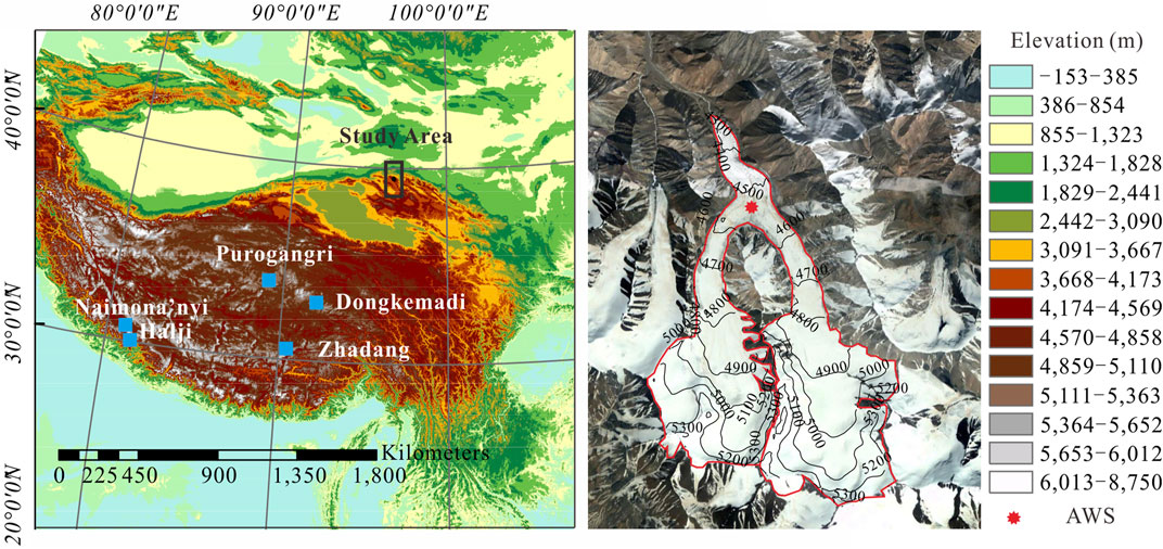
FIGURE 1. The study area on the Qinghai-Tibetan Plateau, including other glaciers where the same model was applied previously as well as Dongkemadi which we use as a validation in this study.

An automatic weather station (AWS) was installed on the glacier at an elevation of 4,550 m (Figures 1, 2). The station monitored air temperature ($\text{T}$), relative humidity (RH), air pressure (p), wind speed (u), shortwave radiation (SW_in and SW_out), and longwave radiation (LW_in and LW_out) between 2010 and 2015 (Table 1; Figure 3). Albedo is determined using radiation measurements around noon to make sure that refraction and diffuse radiation impacts the measurement as little as possible. All data is collected in Beijing time and as a result noon is defined slightly later (12:30–14:30) to correspond to the local situation. A shielded Geonor T-200B precipitation was installed near the AWS, which measured both solid and liquid precipitation. Following previous research on the Tibetan Plateau, 0°C was used as the threshold temperature for distinguishing between solid and liquid precipitation. During the 6-years observation period the average air temperature was −11.0°C. Average relative humidity and wind speed was 46% and 2.8 m s⁻¹ respectively. The mean annual precipitation was 350 mm and snowfall accounts for more than 90% of total precipitation (Figure 3). In addition, wind and temperature data was adjusted to the level of 2 m before running COSIMA. The mass balance was observed by multiple stakes located close to the AWS during 2011, 2012, 2014, and 2015 generally between May and September. It was measured at least once a month during ablation period for each year.

FIGURE 2

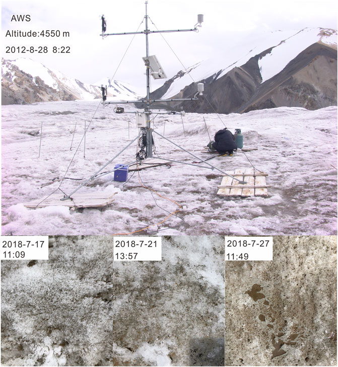
FIGURE 2. The floating AWS installed in 2012. The mass balance stakes are visible in the background and close-up images of the typical glacier surface next to the AWS in 2018 are shown at the bottom of the figure.

TABLE 1

TABLE 1. AWS sensor specifications and installed heights of sensors.

FIGURE 3

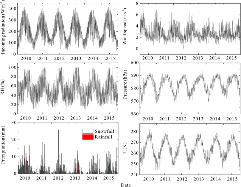
FIGURE 3. Daily meteorological variables between 2010 and 2015. Radiation refers to incoming solar radiation.

Methods

Energy and Mass Balance Model

In this study, we use the Coupled Snowpack and Ice surface energy and Mass balance model (COSIMA) to calculate the energy balance components. The model was successfully used on glaciers of the Tibetan Plateau (Huintjes et al., 2015a; Huintjes et al., 2015b). It combines a surface energy balance (SEB) with a multi-layer subsurface snow and ice model to compute the glacier mass balance (MB) at an hourly resolution. It is computed as follows:

$\text{F}=\text{S}{W}_{in}\cdot \left(1-\alpha \right)+L{W}_{in}+L{W}_{out}+Q_{sens}+Q_{lat}+Q_G(1)$

where $\text{S}{W}_{in}$ is incoming shortwave radiation, $\alpha$ is the surface albedo, $L{W}_{in}$ and $L{W}_{out}$ are incoming and outgoing longwave radiation, $Q_{sens}$ is the turbulent sensible heat flux, $Q_{lat}$ is the turbulent latent heat flux and $Q_G$ is the ground heat flux. Heat flux from liquid precipitation is neglected. Energy fluxes towards the surface have a positive sign. The resulting flux F is equal to $Q_{melt }$ only if the surface temperature ($T_s$) is at the melting point (273.15 K). $T_s$ is calculated iteratively through Eq. 1 from the energy available at the surface. In case $T_s$ exceeds the melting point, it is reset to 273.15 K and the remaining energy flux F equals $Q_{melt. }$

$L{W}_{in}$ and $L{W}_{out}$ are obtained by the Stefan-Boltzmann law. For $L{W}_{in}$, the atmospheric emissivity $\text{ε}$ is calculated after Klok and Oerlemans (2002):

$\text{ε}={\epsilon }_{cs}\cdot \left(1-N^a\right)+{\epsilon }_{cl}\cdot N^a(2)$

where ${\epsilon }_{cs}$ is clear-sky emissivity and ${\epsilon }_{cl}$ is cloud emissivity, $N$ is cloud cover factor, ${\epsilon }_{cs}$ is calculated as follows:

${\epsilon }_{cs}=0.23+b{\left(e/T_{air}\right)}^{1/8}(3)$

where $e$ is water vapour pressure and $T_{air}$ is air temperature. For a, b and ${\epsilon }_{cl}$ we take the values of 2, 0.433 and 0.984, respectively (Klok and Oerlemans, 2002). N is calculated following (Favier et al., 2004):

$\text{N}=1.3-1.4\cdot \left(S{W}_{in}/S{W}_{TOA}\right)(4)$

where $S{W}_{TOA}$ is the top of atmosphere solar irradiance ($\text{W }{m}^{-2})$ and is calculated considering solar constant and geographical position (Kumar et al., 1997).

$S{W}_{TOA}=S_0\left(1+0.0344\cos \left({360}^{°}M/365\right)\right)(5)$

where $S_0$ is the solar constant (1,367 $\text{W}{m}^{-2}$) and M is the day number.

Turbulent heat fluxes $Q_{sens}$ and $Q_{lat}$ are calculated through the standard bulk aerodynamic method (Oerlemans, 2001) between the surface and 1.5 m, using $T_{air}$, RH and wind speed (u) data:

$Q_{sens}={\rho }_{air}{c}_p\frac{k^2}{\text{ln}{\left(\frac{z}{z_0}\right)}^2}u\left(T_{air}-T_s\right)(6)$

$Q_{lat}={\rho }_{air}{L}_{E/S}\frac{k^2}{\text{ln}{\left(\frac{z}{z_0}\right)}^2}u\left(q_{air}-q_s\right)(7)$

${\rho }_{air}$ is air density, calculated from air pressure, $T_{air}$ and specific humidity in 2 m, $c_p$ is specific heat capacity of air (1004.67 J kg⁻¹ K⁻¹), $L_E$ is latent heat of evaporation (2.514 × 106 J kg⁻¹), $L_S$ for sublimation (2.849 × 106 J kg⁻¹), $q_{air}$ and $q_s$ are specific humidity at 1.5 m and at the surface, calculated from RH, p (air pressure) and saturation water vapour pressure. RH is assumed to be 100% at the surface. $k$ is the von Karman constant (0.41), $z$ the instrument height (1.5 m) and $z_0$ the surface roughness length that changes depending on the underlying surface (fresh snow, aged snow, ice) (Mölg et al., 2009):

$Q_G=Q_C+Q_{PS}(8)$

where $Q_C$ is the conductive heat flux and $Q_{PS}$ is the energy flux from penetrating shortwave radiation. $Q_{PS}$ is calculated following Bintanja and Broeke (1995). By

$S_i\left(z\right)=S{W}_{net}\cdot \left(1-\zeta \right)\cdot e^{\beta \cdot z}(9)$

the extinction of net shortwave radiation ($S{W}_{net}$) in the snow or ice layers is parameterized. $S_i$ is the remaining fraction of shortwave radiation reaching down to depth z. In the top model layer, a fraction ζ is absorbed and an exponentially decreasing flux with constant extinction coefficient ß reaches the layers at depth z and increases subsurface temperatures. Thus, $Q_{PS}$ is equal to $S{W}_{net}$ (1-ζ). For ζ and ß we take the values of 0.8 and 2.5 for ice, and 0.9 and 17.1 for snow, respectively (Bintanja and Broeke, 1995).

$Q_C$ is determined from the temperature difference between the surface and the two uppermost subsurface layers and depends on the thermal conductivity (λ) of the medium (ice or snow). λ is calculated from the subsurface density ($\rho$, in kg m⁻³) after Anderson (1976):

$\text{λ}=0.021+2.5\cdot {\left(\rho /1000\right)}^2(10)$

A spin-up time of about 1 year is needed for the subsurface module to adapt to the surrounding conditions. We use our first full year of observations to do so and hence do not compare any mass balance measurements to model outputs from that year.

Albedo Schemes

The original parameterization of surface albedo follows Oerlemans and Knap (1998) where a is determined as a function of snowfall frequency and snow depth:

${\alpha }_{snow}={\alpha }_{firn}+\left({\alpha }_{frsnow}-{\alpha }_{firn}\right)exp\left(t_{snow}/t^{\text{*}}\right)(11)$

$\text{α}={\alpha }_{snow}+{\alpha }_{ice}-{\alpha }_{snow}exp\left(-h/d^{\text{*}}\right)(12)$

${\text{t}}_{\text{snow}}$ is the time since the last snowfall, ${\text{t}}^{\text{*}}$ is a constant for the effect of ageing on snow albedo, h is the snow depth and ${\text{d}}^{\text{*}}$ is a constant for the effect of snow depth on albedo. The original free parameters are adopted according to Huintjes and Schneider (2014): albedo fresh snow (${\text{α}}_{\text{frsnow}}$) = 0.9, albedo firn (${\text{α}}_{\text{firn}}$) = 0.55, albedo ice (${\text{α}}_{\text{ice}}$) = 0.3, ${\text{t}}^{\text{*}}$ = 6 days and ${\text{d}}^{\text{*}}=8\text{cm}$. We will refer to this model as Oerlemans1998 below.

Brock et al. (2000) argued that a more physical representation of the melting process is needed to reproduce albedo values accurately. Using air temperature as a proxy for the atmospheric input they proposed a new parametrization which takes two forms depending on snow depth:

${\alpha }_{snow}=\{\begin{array}{c}0.713-0.112ln{T}_a,snowdepth\ge 0.5 cm w.e.\\ {\alpha }_{ice}+0.442e^{-0.058T_a},snowdepth <0.5 cm w.e.\end{array}(13)$

where $T_a$ is accumulated daily $T_{max}$ above 0°C since the last snowfall (K), $a_{ice}$ is ice albedo (0.3). We will refer to this model as Brock2000 below.

Results

Albedo Simulations

In Figure 4 results of the measured and modelled mean daily albedo values are shown for the measurement period from 2011 to 2015. It is obvious that the Oerlemans1998 model, originally applied in the COSIMA model, fails to reproduce albedo correctly although the simulation curve fluctuates with snowfall. Three crucial shortcomings are apparent.

FIGURE 4

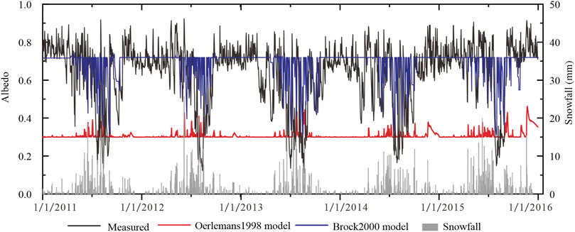
FIGURE 4. Albedo comparison between observation and simulation of Oerlemans1998 and Brock2000 from 2011 to 2015.

First, the initial assumption of an albedo of 0.3 for clean ice does not hold as values are much higher in the region of 0.6–0.8. Huintjes et al. (2015a) note a good match between their model and observations on Zhadang Glacier. There, albedo remains high even longer than on LHG No.12 and just drops briefly down to values around 0.3 during July. More recent research confirms these generally high values but sees a decreasing trend in recent years due to an increase in impurities (Qu et al., 2014). On LHG No.12 albedo only remains high during few weeks between December and January and decreases and increases in between (Figure 4). As rainfall stops after September and temperatures drop rapidly ice remains snow covered and albedo high.

Second, the model predicts a decay that is happening too fast resulting in an immediate return to the chosen value for clean ice while the actual snow depth decay happens much slower (Figure 3). As snow depth simulation and albedo are naturally coupled in the model it is difficult to disentangle that problem. Slightly lower albedo already results in larger $S{W}_{net}$ and therefore increasing $Q_{melt}$ and $Q_{PS}$. This causes snow depth to decrease rapidly (Huintjes and Schneider, 2014). Additionally, accurate snow depth simulations remain a challenge also with other model setups (Stigter et al., 2017; Hedrick et al., 2018; Sauter et al., 2020).

Third, the strong variability of albedo which is apparent during the whole year is not captured by the model, again simply explained by the lack of accurate snow depth data as well as possibly the strong variability that local impurities can cause (Figure 2).

Huintjes and Schneider (2014) had good snow depth data to drive their model. This is missing for LHG No. 12 as the rapid downwasting of the ice surface repeatedly shifts the station and makes surface height measurements largely unusable. We have measurements over a short period of time in 2011 where the station was stable (Figure 5) that visualizes the underestimation of the modelled snow depth. While the model does reproduce measured snow heights just after a snow fall event, the decay of the snowpack is too rapid on nearly all instances. Nevertheless, it should also be noted that observed snow depth also does decay more rapidly than elsewhere. As wind speeds are generally high during the accumulation period fresh snow is eroded quickly.

FIGURE 5

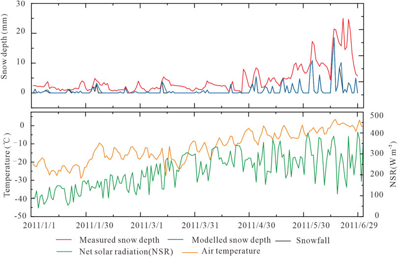
FIGURE 5. Measured and modelled (Oerlemans 1998) snow depth and corresponding meteorological variables in 2011, when snow depth measurements were valid.

Considering that accurate snow depth data remains difficult to obtain in many regions and even individual field sites with climate data, an approach to obtain reliable albedo data that is less sensitive to this variable is called for. Brock et al. (2000) has argued that the accumulated maximum temperature since the last snowfall is a good indicator of snow metamorphosis and proposed a model that does differentiate between deep (> 5 cm) and shallow snow (< 5 cm) but otherwise does not need its precise value as a variable. We apply the model here and the results improve considerably (Figure 4). The R² over the complete model period is 0.23 but is considerably poorer during the accumulation period where the model is not able to reproduce the variability (Figure 4). The error (RMSE and MAE) is 0.16 and 0.11, while the NSE is negative, suggesting that at the daily scale the model still has a poor performance in prediction. We have therefore attempted to develop an algorithm that is able to account for this variability as well during the accumulation period.

Development of New Albedo Parameterization Scheme

Snow albedo is impacted by solar zenith angle, clouds and the snow characteristics (including snow depth, liquid water content, density, particle size, impurities, snow age, surface roughness), as well as the proportion of diffuse reflection to direct radiation (Brock et al., 2000; Wang et al., 2014). We use air temperature and time since last snowfall as model variables. Both variables are also generally easy to obtain in any research site and less prone to sensor malfunction or uncertainty.

We use the idea of a Fourier transformation which is any periodic function that can be decomposed into the sum of several trigonometric functions (Lagerros, 1997) and refer to the new model as FT model below. A similar model has earlier been also applied to develop a solar radiation model (Sun and Kok, 2007). It takes the following form:

$\text{f}\left(x\right)=C+{\displaystyle \sum }_{n=1}^{\infty }\left(a_n\cos \frac{2\pi n}{t}x\right)+b_n\sin \left(\frac{2\pi n}{t}x\right),C\in R(14)$

where t is the period and n is the independent variable. Considering the perturbation effect of snowfall on albedo, the parameterization scheme of albedo is driven predominantly by precipitation. During snowfall events, the default albedo is set to 0.8 as in previous models. When there is no snowfall, albedo is mainly affected by temperature impacting the underlying surface. When the temperature is much below freezing, the state of the snow is relatively stable and remains in a solid form. Similarly, when the temperature is considerably above 0°C, precipitation is liquid. In these two cases, the water phase is relatively stable, and therefore the parameterization scheme only considers temperature as a variable. However, around 0°C, a transient solid-liquid phase occurs which affects the snowpack. In this case, the scheme introduces the parameter of time since last snowfall (m) as well as air temperature. Field data suggest a strong negative relation between albedo and air temperature measurements. Therefore, we propose the following albedo parameterization scheme

$\text{α}=\{\begin{array}{c}100\cos \left(\frac{2\pi T}{365\times 24}\right)-aT\le T_{1}andsnowfall=0\\ 0.8-exp\left(-\frac{T_0}{m\cdot T}\right)T_1<T<T_{2}andsnowfall=0\\ 100\cos \left(\frac{2\pi T}{365\times 24}\right)-cT\ge T_{2}andsnowfall=0\\ 0.8snowfall>0\end{array}(15)$

where $\text{α}$ is albedo, $T$ is air temperature (K), $T_0$ is air temperature at freezing point (273.15 K). $m$ is the time since last snowfall (days). a and c are parameters and T₁ and T₂ are threshold temperatures (K) that are determined from optimization.

We use the data of 2011–2012 to optimize the model parameters and the threshold temperatures that define the transition of the parametrization. The parameters were identified by minimizing RMSE of model output and observations, resulting in a = 97.59 and c = 97.61 and T₁/T₂ = 268/274 K.

Evaluation of the FT Model

In order to verify the simulation accuracy of the new albedo parameterization scheme, statistical indicators of the accumulation period and ablation period of three parameterization schemes were calculated (Table 2). The simulated effect of Oerlemans1998 is naturally poor in any period. Although the accuracy of Brock2000 is higher with lower RMSE (0.08) and MAE (0.06) during the accumulation period, its simulation value remains a constant and the NSE is small (Figure 4; Table 2). The FT model has similar statistics for the ablation period, with a positive but very low NSE suggesting that its predictive power remains low. The very low albedo values (< 0.4) during the ablation season reflected better by the Brock2000 model are not captured by the FT model at the expense of reproducing some of the variability of the accumulation period (Figure 6). During this colder period the new model is able to reproduce the general trend and individual peaks reasonably well (Figure 6; Table 2).

TABLE 2

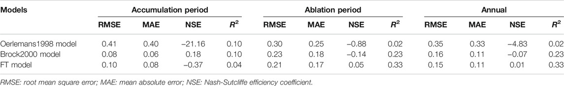
TABLE 2. Basics statistics for all albedo models against observations at the daily scale at LHG No.12 glacier.

FIGURE 6

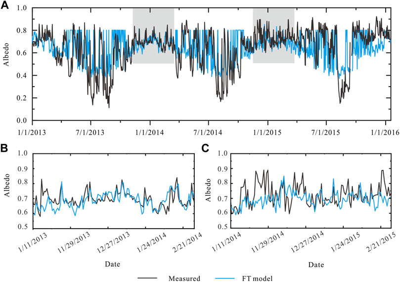
FIGURE 6. (A) Measured albedo and modelled albedo using the FT model during the validation period from 2013 to 2015. The grey rectangles in panel (A) are enlarged in panel (B, C).

The distribution of albedo values for ablation and accumulation period is shown in Figure 7. All models fail to reproduce the large variability especially during the ablation period but both Brock2000 and the FT model are able to reproduce the median and some of the distribution in time. Individual modelled values tend to overestimate in both seasons for the Brock2000 and FT model (Figure 7). When aggregating albedo to weekly values, results improve naturally, but the predictive value for Brock2000 remains low (NSE = 0.01, RMSE = 0.16) and is slightly better for the FT model (NSE = 0.30, RMSE = 0.13).

FIGURE 7

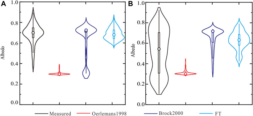
FIGURE 7. Violin plots of simulated albedo during the accumulation (A) and ablation period (B).

Mass Balance Computations

Figure 8 shows the mass balance simulation for all models for four seasons as well as field measurements. While albedo in Oerlemans1998 is generally too constant and low, during the ablation period the actual value is often lower. As a result, the model underestimates melt considerably, even though overall albedo estimates are too low. As can be seen in Figure 4, the simulated albedo of Oerlemans1998 model during the ablation period is relatively high, resulting in lower incoming shortwave radiation. As a result, the glacier melt in the ablation season is lower than the measured value (Figure 8). The RMSE between modelled and measured mass balance is 0.52 m w.e. over all years, varying from 0.24 m w.e. in 2015 to 0.76 m w.e. in 2012.

FIGURE 8

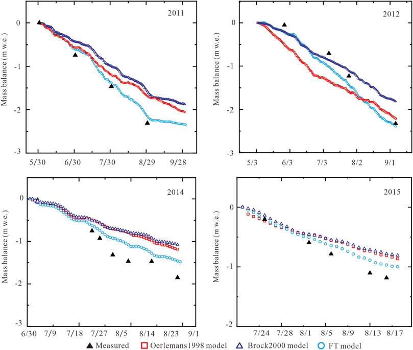
FIGURE 8. Comparison of mass balance using original and new albedo parameterization schemes. Note different time periods for different years based on available data.

Although albedo variability is reproduced much better for the Brock2000 model than the Oerlemans1998 approach, this translates only into slightly improved mass balance estimates (Figure 8). The RMSE for Brock2000 decreases relatively little to 0.39 m w.e. (0.23 and 0.52 m w.e. in 2012 and 2014 respectively), mainly due to large remaining errors during the beginning of the melt season where melt is underestimated as albedo drops earlier in the season than modelled (Figure 4). This is improved for the new scheme (Figure 6) and overestimations become overall lower (Figure 8). Additional potential sources of error are likely within the turbulent fluxes which are difficult to capture accurately. The FT model, with albedo calibrated for 2011 and 2012, reproduces mass loss very well and has a considerably lower error than the other models over all years (RMSE = 0.19 m w.e., Figure 8). Naturally, the error is lower in the years where the albedo scheme was calibrated (0.13 and 0.17 m w.e. in 2011 and 2012 respectively), and slightly higher in the other 2 years (0.27 and 0.14 m w.e. in 2014 and 2015 respectively). This suggests that getting albedo right alone is likely to result in good estimates of mass loss with the energy balance approach.

Validation on Dongkemadi Glacier

In order to verify the transferability of the new albedo parameterization scheme, the data of Dongkemadi Glacier located in the Tanggula mountains in the middle of the Qinghai-Tibet Plateau was used. The measurements are from January 1 to December 31, 2012, obtained at 5,700 m a.s.l. and are previously unpublished.

As for LH No. 12 the Oerlemans1998 model fails to capture the magnitude or variability of the observed albedo. Due to the cold temperatures on Dongkemadi Glacier and again a lack of accurate snow depth data the Brock2000 fails to reproduce most of the observed variability. Using the parameters found at LHG No. 12 for the FT model provides reasonable variability during the ablation period which the other models fail to reproduce at any time (Figure 9). However, the predictive power of all models is very poor. During the accumulation period the RMSE of FT model, Oerlemans1998 model and Brock2000 model are −0.11, 0.22, and 0.11 respectively. For the ablation period the RMSE improves to 0.13, 0.23, and 0.09 but even for the FT model the NSE remains low (0.12) and negative for other models.

FIGURE 9

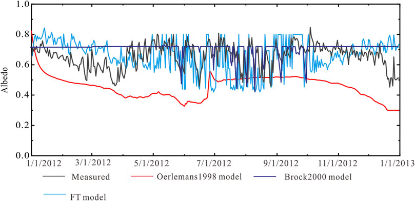
FIGURE 9. Comparison of simulation results of different models with actual measurements on Dongkemadi Glacier.

Discussion

Our results show that the choice of albedo parametrization for an accurate estimation of mass balance with an energy balance model is crucial. Lacking accurate snow depth data, the COSIMA model fails to reproduce albedo and consequently mass balance with the original scheme. As the albedo scheme is dependent on snow depth data generated by the model its performance is impacted by the ability of COSIMA to reproduce snow height accurately. This the model fails to do in our case (Figure 5). Similarly, measurements are prone to large uncertainties due to the rapid downwasting of the surface which in extreme cases in July and August exceeded 5 cm day⁻¹ at the measured stakes. Therefore, we believe it is prudent to rely on parametrizations that do not rely on accurate daily snow depth values.

Additionally, as the AWS is located in the lower ablation area of the glacier, snow disappears rapidly and no continuous snowpack develops, as evidenced from satellite imagery. The ice surface is hence mostly exposed, which exhibits a rapidly changing surface morphology through melt as well possibly constantly shifting deposits of impurities, that can also be accumulated and transported away by melt water (Figure 2). We suspect that the original parametrization is simply not very suitable for this environment.

The Brock2000 model already provides much better results than the original parametrization and focusing on the ablation period only reproduces the magnitude of albedo generally well. The RMSE for the entire year is reduced from 0.35 to just 0.16, compared to the original parametrization. However, it cannot be solved when the maximum temperature is lower than 0°C, which happens in the region throughout the accumulation and at times even the ablation season (Brock et al., 2000). Therefore, Brock2000 fails to reproduce the strong variability of albedo during the accumulation period. The new FT model proposed here, calibrated for 2 years of the data series, improves the statistics only slightly but is notably able to provide variability in the cold period as well. While mass balance computations using the uncalibrated Brock2000 model already improve, reducing the RMSE from 0.52 to 0.39 m w.e., using the calibrated FT model reduces this even further to 0.19 m w.e. This strongly suggests that calibrating parameters for the specific location remains crucial. This is further supported by applying the same FT model with the same parameters on another glacier on the Tibetan Plateau.

While the variability introduced matches the observations overall, the model has little predictive power on the daily scale. To improve, it would need to be recalibrated at the same site. A different model has previously been developed at the nearby Qiyi Glacier (108 km west of LHG No. 12) in the Qilian mountains (Jiang et al., 2011). The model uses temperature, days since last snowfall and cloudiness as variables and works well on the Qiyi Glacier but depends on 6 different calibrated parameters. It does less so at LHG No. 12 (Figure 10). While variability is introduced, the magnitude is considerably off and recalibration would again be necessary.

FIGURE 10

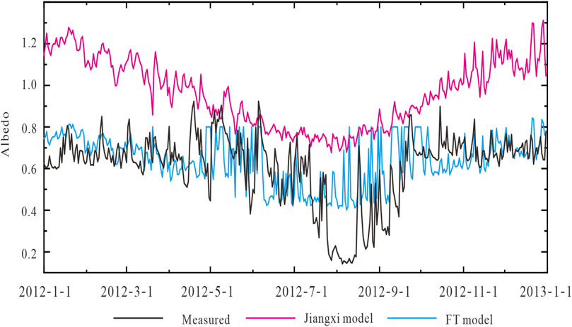
FIGURE 10. Simulation results of Jiangxi model and FT model compared with the actual measurements on LHG glacier No.12.

The difference in albedo magnitude and variability between the glaciers in the region emphasizes the importance to carefully choose parametrizations for glacier scale studies and in the best case calibrate them to the local surface properties and climate (Bamber and Payne, 2004). While the model developed here for LHG No.12 works very well to generate reasonable mass balance estimates and can be transferred in time without a strong loss in accuracy and also reproduces the strong variability of albedo in both accumulation and ablation period, transfer to another location is still not straightforward. Even the well-established Brock2000 model however improves albedo estimates considerably for the ablation period alone even without any site-specific recalibration.

We argue that the failure of the Oerlemans1998 model for the case of the LHG No.12 Glacier is due to the lack of accurate snow depth data. Glaciers previously studied with the COSIMA model include Zhadang Glacier on the southern central TP, Halji Glacier in the western Himalayas, Naimona’nyi Glacier on the south western TP, Purogangri Ice Cap on the central TP and a glacier in the Muztagh Ata Shan on the north western TP (Figure 1), which are affected by the westerly winds and the Indian monsoon (Huintjes and Schneider, 2014). However, LHG No. 12 is located to the northeast of the Qinghai-Tibet plateau, controlled by the east Asian season (Domrös and Peng, 1988; Chen et al., 2019). Studies have shown that the average content of glacial black carbon on the edge of the Qinghai-Tibet Plateau is much higher than that of inland areas (Li, 2017; Li, 2020). That could explain some of the strong variability that is difficult to capture with an albedo model dependent only on air temperature.

A striking feature of observed albedo on LHG No 12. and Dongkemadi is the strong daily variability which is caused largely by the presence of impurities transported to the glacier surface but also the different moisture sources of the dominating precipitation for each glacier. Their presence obviously has a strong effect on the albedo of the overall glacier surface. None of the models so far are able to account for such variables.

Apart from the fact that the lack of accurate snow depth measurements likely explains the failure of previously used models in our case, we have also investigated potential differences in atmospheric drivers that could explain the strong daily variability in albedo on LHG No.12 as well as Dongkemadi Glacier. In order to analyze the source of air masses, the backward trajectory during August 2012, when monsoon is active, of LHG Glacier No. 12 and Zhadang Glacier was calculated by the Meteoinfo software (http://www.meteothink.org/) (Wang, 2014). We used NCEP/NCAR global analysis data (air pressure, temperature, relative humidity, vertical and horizontal wind speed) provided by NOAA (with a resolution of 2.5° × 2.5°) for model forcing (https://www.ready.noaa.gov/HYSPLIT.php). The dominant source region at LHG Glacier No. 12 is from the continental area over the relatively densely populated Gansu province. At Zhadang Glacier dominant source areas are over the Central Tibetan Plateau. Previous work has shown that a high value of light-absorbing impurities, including both black carbon (BC) and mineral dust (MD) is present on LHG Glacier No. 12 (Li, 2020). The BC and MD contents of LHG Glacier No. 12 are much higher than that of Dongkemadi Glacier and Zhadang Glacier, with the lowest measurements taken at Zhadang Glacier (Li, 2017). This presence of impurities could explain the strong temporal variability of albedo on glaciers like LHG No. 12, especially in the ablation areas where the ice is exposed for a large part of the year.

Conclusion

In this paper we show how a mass and energy balance model applied on a glacier in the Qilian Shan, on the northern fringes of the Tibetan Plateau, fails due to the use of an albedo scheme that is dependent on accurate snow depth data that is not available in our case and in many other field sites. Not only does the original albedo parametrization underestimate albedo continuously but also fails to reproduce a strong daily variability present on this glacier as well as another validation site. Applying another well-established model that only relies on air temperature measurements and the time to last snowfall considerably improves results. While it still fails to reproduce the variability of the accumulation period, it is in the right order of magnitude and reproduces some of the variability in the ablation period. Applying a new model developed and calibrated for this location that equally only relies on air temperature and time since last snow fall further slightly improves results, but more importantly improves mass balance estimates. While the original scheme results in a RMSE of the modelled mass balance against stake measurements of 0.52 m w.e. from measurements over four melt seasons, the new approach reduces this error to just 0.19 m w.e. However the new model has been calibrated for this specific site, while for the Brock2000 model, where the RMSE is reduced to 0.39 m w.e., we relied on the original parametrization derived in the European Alps. This suggests that the Brock2000 model, without any recalibration of parameters is a more reasonable choice to determine albedo, specifically in the ablation area of glaciers. On the other hand, the FT model introduced here fails to provide significant improvement to reproduce daily albedo during the ablation period nor is it transferable in space. Using this model on another glacier on the Tibetan Plateau shows that the same parameters produce accurate average estimates considering the whole season but fail to reproduce accurate daily albedo measurements. This can be explained by a different temperature regime in the second location, a considerably colder climate. Its advantage lies in the ability to reproduce albedo variability during very cold periods, where Brock2000 fails to provide variability as well as the fact that it does not rely on snow depth data.

In the present model we do not consider impurities and moisture controls on melt. Both vary considerably in the region and have been shown to be of great importance to changing melt patterns already. They are of special importance in the ablation area where surfaces tend to be of heterogenous composition and undergo rapid morphological change. Studies that investigate future mass loss in the region should consider the effect these impurities have on the development of surface albedo, including their potential change with climate change as well as a potential change in airborne particles due to local desiccation as well as direct anthropogenic sources.

Data Availability Statement

Inquiries regarding data can be directed to the corresponding author.

Author Contributions

Writing—original draft preparation, LW; conceptualization, LW and DZ; methodology, LW, JS, and JC; software, DZ; validation, JS; formal analysis, LW and JS; investigation, LW and JC; resources, XQ; data curation, XH, YuL, YaL, and ZJ; Writing—review, analysis and editing, LW, JS; visualization, LW and DZ; supervision, XQ; project administration, XQ; funding acquisition, XQ.

Funding

Financial support is gratefully acknowledged to the Second Scientific Expedition Project on the Qinghai-Tibet Plateau (2019QZKK020103) as well as the Strategic Leading Science and technology project of Chinese Academy of Sciences (XDA2002010202); Major projects of Natural Science Foundation of Gansu Province (18JR2RA002). The views and interpretations in this publication are those of the authors and they are not necessarily attributable to their organizations.

Conflict of Interest

The authors declare that the research was conducted in the absence of any commercial or financial relationships that could be construed as a potential conflict of interest.

Publisher’s Note

All claims expressed in this article are solely those of the authors and do not necessarily represent those of their affiliated organizations, or those of the publisher, the editors and the reviewers. Any product that may be evaluated in this article, or claim that may be made by its manufacturer, is not guaranteed or endorsed by the publisher.

Acknowledgments

Thanks to Dr. Miao Zhong for her technical support with the Meteoinfo software. We thank three reviewers and Editor Dr. Baojuan Huai for the provided comments that have helped us improve the manuscript substantially.

References

Anderson, E. A. (1976). A point Energy and Mass Balance Model of a Snow Cover. San Francisco: Stanford University.

Google Scholar

J. L. Bamber,, and A. J. Payne (Editors) (2004). Mass Balance of the Cryosphere: Observations and Modelling of Contemporary and Future Changes (Cambridge: Cambridge University Press). doi:10.1017/CBO9780511535659

CrossRef Full Text | Google Scholar

Bintanja, R., and Broeke, M. R. V. D. (1995). The Surface Energy Balance of Antarctic Snow and Blue Ice. J. Appl. Meteorol. 34, 902–926. doi:10.1175/1520-0450(1995)034<0902:tseboa>2.0.co;2

CrossRef Full Text | Google Scholar

Brock, B. W., Willis, I. C., and Sharp, M. J. (2000). Measurement and Parameterization of Albedo Variations at Haut Glacier d'Arolla, Switzerland. J. Glaciol. 46, 675–688. doi:10.3189/172756500781832675

CrossRef Full Text | Google Scholar

Brun, F., Berthier, E., Wagnon, P., Kääb, A., and Treichler, D. (2017). A Spatially Resolved Estimate of High Mountain Asia Glacier Mass Balances from 2000 to 2016. Nat. Geosci 10, 668–673. doi:10.1038/ngeo2999

PubMed Abstract | CrossRef Full Text | Google Scholar

Chen, L., Duan, K., Wang, N., Jiang, X., He, J., Song, G., et al. (2007). Characteristics of the Surface Energy Balance of the Qiyi Glacier in Qilian Mountains in Melting Season. J. Glaciol. Geoc Ryology 29, 882–888.

Google Scholar

Chen, F., Fu, B., Xia, J., Wu, D., Wu, S., Zhang, Y., et al. (2019). Major Advances in Studies of the Physical Geography and Living Environment of China during the Past 70 Years and Future Prospects. Sci. China Earth Sci. 62, 1665–1701. doi:10.1007/s11430-019-9522-7

CrossRef Full Text | Google Scholar

Ding, B., Yang, K., Yang, W., He, X., Chen, Y., La, Z., et al. (2017). Development of a Water and Enthalpy Budget-Based Glacier Mass Balance Model (WEB-GM) and its Preliminary Validation. Water Resour. Res. 53, 3146–3178. doi:10.1002/2016WR018865

CrossRef Full Text | Google Scholar

Domrös, M., and Peng, G. (1988). The Climate of China. Berlin Heidelberg: Springer-Verlag. doi:10.1007/978-3-642-73333-8

CrossRef Full Text | Google Scholar

Dunkle, R. V., and Bevans, J. T. (1956). An Approximate Analysis of the Solar Reflectance and Transmittance of a Snow Cover. J. Meteorol. 13, 212–216. doi:10.1175/1520-0469(1956)013<0212:aaaots>2.0.co;2

CrossRef Full Text | Google Scholar

Favier, V., Wagnon, P., Chazarin, J.-P., Maisincho, L., and Coudrain, A. (2004). One-Year Measurements of Surface Heat Budget on the Ablation Zone of Antizana Glacier 15, Ecuadorian Andes. J. Geophys. Res. 109 (D18). doi:10.1029/2003JD004359

CrossRef Full Text | Google Scholar

Fujita, K., Ohta, T., and Ageta, Y. (2007). Characteristics and Climatic Sensitivities of Runoff from a Cold-Type Glacier on the Tibetan Plateau. Hydrol. Process. 21, 2882–2891. doi:10.1002/hyp.6505

CrossRef Full Text | Google Scholar

Gardner, A. S., and Sharp, M. J. (2010). A Review of Snow and Ice Albedo and the Development of a New Physically Based Broadband Albedo Parameterization. J. Geophys. Res. 115 (F1). doi:10.1029/2009JF001444

CrossRef Full Text | Google Scholar

Guo, W., Liu, S., Xu, J., Wu, L., Shangguan, D., Yao, X., et al. (2015). The Second Chinese Glacier Inventory: Data, Methods and Results. J. Glaciol. 61, 357–372. doi:10.3189/2015JoG14J209

CrossRef Full Text | Google Scholar

Hedrick, A. R., Marks, D., Havens, S., Robertson, M., Johnson, M., Sandusky, M., et al. (2018). Direct Insertion of NASA Airborne Snow Observatory‐Derived Snow Depth Time Series into the iSnobal Energy Balance Snow Model. Water Resour. Res. 54, 8045–8063. doi:10.1029/2018WR023190

CrossRef Full Text | Google Scholar

Hock, R., and Holmgren, B. (2005). A Distributed Surface Energy-Balance Model for Complex Topography and its Application to Storglaciären, Sweden. J. Glaciol. 51, 25–36. doi:10.3189/172756505781829566

CrossRef Full Text | Google Scholar

Huintjes, E., and Schneider, C. (2014). Energy and Mass Balance Modelling for Glaciers on the Tibetan Plateau : Extension, Validation and Application of a Coupled Snow and Energy Balance Model. PhD Thesis. Aachen: RWTH Aachen University.

Google Scholar

Huintjes, E., Neckel, N., Hochschild, V., and Schneider, C. (2015a). Surface Energy and Mass Balance at Purogangri Ice Cap, Central Tibetan Plateau, 2001-2011. J. Glaciol. 61, 1048–1060. doi:10.3189/2015JoG15J056

CrossRef Full Text | Google Scholar

Huintjes, E., Sauter, T., Schröter, B., Maussion, F., Yang, W., Kropáček, J., et al. (2015b). Evaluation of a Coupled Snow and Energy Balance Model for Zhadang Glacier, Tibetan Plateau, Using Glaciological Measurements and Time-Lapse Photography. Arct. Antarct. Alp. Res. 47, 573–590. doi:10.1657/AAAR0014-073

CrossRef Full Text | Google Scholar

Immerzeel, W. W., Lutz, A. F., Andrade, M., Bahl, A., Biemans, H., Bolch, T., et al. (2020). Importance and Vulnerability of the World’s Water Towers. Nature 577, 364–369. doi:10.1038/s41586-019-1822-y

PubMed Abstract | CrossRef Full Text | Google Scholar

Jansson, P., Hock, R., and Schneider, T. (2003). The Concept of Glacier Storage: A Review. J. Hydrol. 282, 116–129. doi:10.1016/S0022-1694(03)00258-0

CrossRef Full Text | Google Scholar

Jiang, X., Wang, N., He, J., Song, G., Yang, S., and Wu, X. (2011). A Study of Parameterization of Albed on the Qiyi Glacier in Qillian Montains, China. J. Glaciol. Geoc Ryology 33, 30–37.

Google Scholar

Kääb, A., Berthier, E., Nuth, C., Gardelle, J., and Arnaud, Y. (2012). Contrasting Patterns of Early Twenty-First-Century Glacier Mass Change in the Himalayas. Nature 488, 495–498. doi:10.1038/nature11324

PubMed Abstract | CrossRef Full Text | Google Scholar

Klok, E. J., and Oerlemans, J. (2002). Model Study of the Spatial Distribution of the Energy and Mass Balance of Morteratschgletscher, Switzerland. J. Glaciol. 48, 505–518. doi:10.3189/172756502781831133

CrossRef Full Text | Google Scholar

Konzelmann, T., and Braithwaite, R. J. (1995). Variations of Ablation, Albedo and Energy Balance at the Margin of the Greenland Ice Sheet, Kronprins Christian Land, Eastern north Greenland. J. Glaciol. 41, 174–182. doi:10.3189/S002214300001786X

CrossRef Full Text | Google Scholar

Kukla, G. J., and Kukla, H. J. (1974). Increased Surface Albedo in the Northern Hemisphere. Science 183, 709–714. doi:10.1126/science.183.4126.709

PubMed Abstract | CrossRef Full Text | Google Scholar

Kumar, L., Skidmore, A. K., and Knowles, E. (1997). Modelling Topographic Variation in Solar Radiation in a GIS Environment. Int. J. Geographical Inf. Sci. 11, 475–497. doi:10.1080/136588197242266

CrossRef Full Text | Google Scholar

Lagerros, J. S. V. (1997). Thermal Physics of Asteroids. III. Irregular Shapes and Albedo Variegations. Astron. Astrophys. 325, 1226–1236.

Google Scholar

Li, Y.-J., Ding, Y.-J., Shangguan, D.-H., and Wang, R.-J. (2019). Regional Differences in Global Glacier Retreat from 1980 to 2015. Adv. Clim. Change Res. 10, 203–213. doi:10.1016/j.accre.2020.03.003

CrossRef Full Text | Google Scholar

Li, X. (2017). Characteristics of Light-Absorbing Impurities in the Surface Snow/Ice on the Tibetan Plateau Glaciers and its Potential Impact on Glacier Melt: An Investigative on the Xiao Dongkemadi and Zhadang Glacier. PhD Thesis. Beijing: University of Chinese Academy of Sciences.

Google Scholar

Li, Y. (2020). Physical Properties of Black Carbon in the Third Polar Glaciers and Their Effects on Albedo Reduction. PhD Thesis. Beijing: University of Chinese Academy of Sciences.

Google Scholar

Liang, L., Cuo, L., and Liu, Q. (2018). The Energy and Mass Balance of a Continental Glacier: Dongkemadi Glacier in central Tibetan Plateau. Sci. Rep. 8, 12788. doi:10.1038/s41598-018-31228-5

PubMed Abstract | CrossRef Full Text | Google Scholar

Liu, Y., Qin, X., Du, W., Sun, W., and Hou, D. (2010). Analysis on Movement Characteristics of Laohugou Glacier No. 12 in Qilian Mountains. J. Glaciol. Geoc Ryology 32, 475–479.

Google Scholar

Liu, Y., Qin, X., Zhang, T., Zhang, M., and Du, W. (2012). Variation of the Ningchan River Glacier No. 3 in the Linglonging Range, East Qilian Montains. J. Glaciol. Geoc Ryology 34, 1031–1036.

Google Scholar

Liu, L., Jiang, L., Sun, Y., Wang, H., Sun, Y., and Xu, H. (2019). Diurnal Fluctuations of Glacier Surface Velocity Observed with Terrestrial Radar Interferometry at Laohugou No. 12 Glacier, Western Qilian Mountains, China. J. Glaciol. 65, 239–248. doi:10.1017/jog.2019.1

CrossRef Full Text | Google Scholar

Liu, J., Chen, R., and Han, C. (2020). Spatial and Temporal Variations in Glacier Aerodynamic Surface Roughness during the Melting Season, as Estimated at the August-One Ice Cap, Qilian Mountains, China. The Cryosphere 14, 967–984. doi:10.5194/tc-14-967-2020

CrossRef Full Text | Google Scholar

Mölg, T., Cullen, N. J., Hardy, D. R., Winkler, M., and Kaser, G. (2009). Quantifying Climate Change in the Tropical Midtroposphere over East Africa from Glacier Shrinkage on Kilimanjaro. J. Clim. 22, 4162–4181. doi:10.1175/2009JCLI2954.1

CrossRef Full Text | Google Scholar

Oerlemans, J., and Knap, W. H. (1998). A 1 Year Record of Global Radiation and Albedo in the Ablation Zone of Morteratschgletscher, Switzerland. J. Glaciol. 44, 231–238. doi:10.1017/s0022143000002574

CrossRef Full Text | Google Scholar

Oerlemans, J. (2001). Glaciers and Climate Change. Boca Raton: CRC Press.

Google Scholar

Qin, X., Cui, X., Du, W., Dong, Z., Ren, J., and Chen, J. (2015). Variations of the alpine Precipitation from an Ice Core Record of the Laohugou Glacier basin during 1960-2006 in Western Qilian Mountains, China. J. Geogr. Sci. 25, 165–176. doi:10.1007/s11442-015-1160-4

CrossRef Full Text | Google Scholar

Qing, W., Han, C., and Liu, J. (2018). Surface Energy Balance of Bayi Ice Cap in the Middle of Qilian Mountains, China. J. Mt. Sci. 15, 1229–1240. doi:10.1007/s11629-017-4654-y

CrossRef Full Text | Google Scholar

Qu, B., Ming, J., Kang, S.-C., Zhang, G.-S., Li, Y.-W., Li, C.-D., et al. (2014). The Decreasing Albedo of the Zhadang Glacier on Western Nyainqentanglha and the Role of Light-Absorbing Impurities. Atmos. Chem. Phys. 14, 11117–11128. doi:10.5194/acp-14-11117-2014

CrossRef Full Text | Google Scholar

Sakai, A., Fujita, K., Duan, K., Pu, J., Nakawo, M., and Yao, T. (2006). Five Decades of Shrinkage of July 1st Glacier, Qilian Shan, China. J. Glaciol. 52, 11–16. doi:10.3189/172756506781828836

CrossRef Full Text | Google Scholar

Sauter, T., Arndt, A., and Schneider, C. (2020). COSIPY v1.3 - an Open-Source Coupled Snowpack and Ice Surface Energy and Mass Balance Model. Geosci. Model. Dev. 13, 5645–5662. doi:10.5194/gmd-13-5645-2020

CrossRef Full Text | Google Scholar

Sicart, J. E., Hock, R., and Six, D. (2008). Glacier Melt, Air Temperature, and Energy Balance in Different Climates: The Bolivian Tropics, the French Alps, and Northern Sweden. J. Geophys. Res. 113 (D24). doi:10.1029/2008JD010406

CrossRef Full Text | Google Scholar

Six, D., Wagnon, P., Sicart, J. E., and Vincent, C. (2009). Meteorological Controls on Snow and Ice Ablation for two Contrasting Months on Glacier de Saint-Sorlin, France. Ann. Glaciol. 50, 66–72. doi:10.3189/172756409787769537

CrossRef Full Text | Google Scholar

Stigter, E. E., Wanders, N., Saloranta, T. M., Shea, J. M., Bierkens, M. F. P., and Immerzeel, W. W. (2017). Assimilation of Snow Cover and Snow Depth into a Snow Model to Estimate Snow Water Equivalent and Snowmelt Runoff in a Himalayan Catchment. The Cryosphere 11, 1647–1664. doi:10.5194/tc-11-1647-2017

CrossRef Full Text | Google Scholar

Sun, Y., and Kok, R. (2007). A Solar Radiation Model with a Fourier Transform Approach. Can. Biosyst. Eng. 49, 7.

Google Scholar

Sun, W., Qin, X., Ren, J., Yang, X., Zhang, T., Liu, Y., et al. (2012). The Surface Energy Budget in the Accumulation Zone of the Laohugou Glacier No. 12 in the Western Qilian Mountains, China, in Summer 2009. Arct. Antarct. Alp. Res. 44, 296–305. doi:10.1657/1938-4246-44.3.296

CrossRef Full Text | Google Scholar

Sun, W., Qin, X., Du, W., Liu, W., Liu, Y., Zhang, T., et al. (2014). Ablation Modeling and Surface Energy Budget in the Ablation Zone of Laohugou Glacier No. 12, Western Qilian Mountains, China. Ann. Glaciol. 55, 111–120. doi:10.3189/2014AoG66A902

CrossRef Full Text | Google Scholar

van de Wal, R. S. W. (1996). Mass-Balance Modelling of the Greenland Ice Sheet: A Comparison of an Energy-Balance and a Degree-Day Model. Ann. Glaciol. 23, 36–45. doi:10.3189/S0260305500013239

CrossRef Full Text | Google Scholar

Wang, J., Cui, Y., He, X., Zhang, J., and Yan, S. (2015). Surface Albedo Variation and its Influencing Factors Over Dongkemadi Glacier, Central Tibetan Plateau. Adv. Meteorology 2015, e852098. doi:10.1155/2015/852098

CrossRef Full Text | Google Scholar

Wang, J., Ye, B., Cui, Y., He, X., and Yang, G. (2014). Spatial and Temporal Variations of Albedo on Nine Glaciers in Western China from 2000 to 2011. Hydrol. Process. 28 (9), 3454–3465. doi:10.1002/hyp.9883

CrossRef Full Text | Google Scholar

Wang, Y., Zhang, T., Ren, J., Qin, X., Liu, Y., Sun, W., et al. (2018). An Investigation of the Thermomechanical Features of Laohugou Glacier No. 12 on Qilian Shan, Western China, Using a Two-Dimensional First-Order Flow-Band Ice Flow Model. The Cryosphere 12, 851–866. doi:10.5194/tc-12-851-2018

CrossRef Full Text | Google Scholar

Wang, Z. (1981). Glacier Inventory of China I: Qilian Mountains. Lanzhou: Lanzhou Institute of Glaciology and Cryopedology.

Google Scholar

Wang, Y. Q. (2014). MeteoInfo: GIS Software for Meteorological Data Visualization and Analysis. Met. Apps 21, 360–368. doi:10.1002/met.1345

CrossRef Full Text | Google Scholar

Wiscombe, W. J., and Warren, S. G. (1980). A Model for the Spectral Albedo of Snow. I: Pure Snow. J. Atmos. Sci. 37, 2712–2733. doi:10.1175/1520-0469(1980)037<2712:amftsa>2.0.co;2

CrossRef Full Text | Google Scholar

Yang, X., Qin, D., Zhang, Y., Kang, S., Qin, X., and Liu, H. (2010). Seasonal Characteristics of Surface Radiation Fluxes on the East Rongbuk Glacier in the Mt.Everest Region. Acta Meteorol. Sin. 24, 680–698.

Google Scholar

Yang, W., Guo, X., Yao, T., Yang, K., Zhao, L., Shenghai, L., et al. (2011). Summertime Surface Energy Budget and Ablation Modeling in the Ablation Zone of a Martime Tibetan Glacier. J. Geophys. Res. 116, D14116. doi:10.1029/2010JD015183

CrossRef Full Text | Google Scholar

Yao, T., Thompson, L., Yang, W., Yu, W., Gao, Y., Guo, X., et al. (2012). Different Glacier Status with Atmospheric Circulations in Tibetan Plateau and Surroundings. Nat. Clim. Change 2, 663–667. doi:10.1038/nclimate1580

CrossRef Full Text | Google Scholar

Zhang, Y., Yao, T., and Pu, J. (1996). Energy Budget at ELA on Dongkemadi Glacier in the Tonggula M Ts. Tibetan Plateau. J. Glaciol. Geocryol. 18, 10–19.

Google Scholar

Zhang, Y., Liu, S., and Ding, Y. (2007). Glacier Meltwater and Runoff Modelling, Keqicar Baqi Glacier,southwestern Tien Shan, China. J. Glaciol. 53, 91–98. doi:10.3189/172756507781833956

CrossRef Full Text | Google Scholar

Zhang, Y., Liu, S., Shangguan, D., Li, J., and Zhao, J. (2012). Thinning and Shrinkage of Laohugou No. 12 Glacier in the Western Qilian Mountains, China, from 1957 to 2007. J. Mt. Sci. 9, 343–350. doi:10.1007/s11629-009-2296-4

CrossRef Full Text | Google Scholar

Zhang, G., Kang, S., Fujita, K., Huintjes, E., Xu, J., Yamazaki, T., et al. (2013). Energy and Mass Balance of Zhadang Glacier Surface, Central Tibetan Plateau. J. Glaciol. 59, 137–148. doi:10.3189/2013JoG12J152

CrossRef Full Text | Google Scholar

Zhang, Y., Kang, S., Cong, Z., Schmale, J., Sprenger, M., Li, C., et al. (2017). Light-Absorbing Impurities Enhance Glacier Albedo Reduction in the Southeastern Tibetan Plateau. J. Geophys. Res. Atmospheres 122, 6915–6933. doi:10.1002/2016JD026397

CrossRef Full Text | Google Scholar