Effect of Velocity Anisotropy in Shale on the Acoustic Emission Events Matching and Location

1 Introduction

Seismic source location is important in earthquake research, fracturing monitoring, and acoustic emission (AE) experiment. Triggering events can be located by minimizing an objective function in terms of the difference between observed and theoretical arrival times (Geiger, 1912; Ge, 2013; Wuestefeld et al., 2018). The reliable location of an event depends on an accurate velocity model. Current source location methods assume homogenous and isotropic velocity models (King and Talebi, 2007; Zhou et al., 2017). However, shale is observed to have strong anisotropy caused by preferentially orientated clay platelets and other integrated factors on a small scale (Vernik and Nur, 1992; Lonardelli et al., 2007; Zhang, 2017; Zhang et al., 2017). Anisotropic shale can be modeled as a VTI (vertical transverse isotropy) medium in which the velocity of the acoustic wave perpendicular to the shale bedding is less than the velocity parallel to the shale bedding. The magnitude of shale anisotropy can be up to 40%, and thus the effect of anisotropy must be taken into account in source location and event-matching.

Event-matching obtaining valid AE signals is a necessary procedure to locate the source. Valid AE signals mean those signals are from the same source and are received by at least four receivers because four unknown source parameters including the location coordinates (x₀, y₀, z₀) and the origin time (t₀) need to be determined. Accurate events matching can be difficult since signals contain false AE detections, electronic noise, anthropogenic noise, and other signals (López Comino et al.,2017). In addition, AE signals can be mixed with boundary reflections or signals from other sources. The cross-correlation event-matching method uses the similarity of signals received by each channel from the same source (Gibbons and Ringdal, 2006; Song et al., 2010). Another effective method for event-matching is based on the maximum time difference between the earliest and latest arrivals (Feng et al., 2019). The maximum time acts as a threshold and is usually calculated in terms of isotropy. However, sensors are placed in geometries with a wide range of directions, and therefore the presence of anisotropy can have a large impact on the results of event-matching.

An inaccurate velocity model is another factor that leads to uncertainty in locating an event. Current AE and microseismic methods for determining the location of the source often assume that acoustic waves propagate in straight lines at a constant velocity for all sensors, and the location of the source is determined by the average wave velocity or vertical velocity determined from well-logging data (King and Talebi, 2007; Zhou et al., 2017). Thus, the effect of anisotropy must also be included in the source location. The importance of including VTI corrections, when detecting microseismic events, was shown by King and Talebi (2007) and Maxwell et al. (2010). A variable velocity method is proposed to address the location problem of a complex multilayer velocity model (Li and Qi, 2009). Van Dok et al. (2011) discussed some of the fundamental elements of how HTI (horizontal transverse isotropic) and VTI affect the correct location of microseismic imaging points. However, these methods allow obtaining anisotropic parameters using control measurements, cross-well measurement using three-component sensors, and advanced dipole sonic, which is mainly applicable to field microseismic data and makes it difficult to obtain anisotropic parameters in AE experiments in the laboratory; therefore, we use a core measurement method to obtain an anisotropic velocity model. An improved Geiger’s method is proposed that corrects the anisotropic velocity instead of using a constant velocity during each iteration.

In this article, we first perform ultrasonic measurements on a shale sample from the lower Silurian shale formation in the southern Sichuan Basin to investigate its elastic properties. An acoustic emission experiment is then carried out on a shale sample. The number of located sources using traditional event-matching and Geiger’s method is incompatible with the X-ray image of the fracture. To address this issue, we study the effect of anisotropy on event-matching and propose an improved event-matching method based on a triangulation method considering velocity anisotropy. The newly proposed matching method greatly improves data-processing efficiency by reducing invalid redundant AE events. Finally, we propose an improved Geiger’s method by taking into account velocity anisotropy and verify the accuracy of the location results based on a CT scan.

2 Ultrasonic Measurements of a Shale Sample

Shale samples are collected from an outcrop of the Longmaxi formation in Wulong County, Chongqing City (Figure 1A,B). The density and porosity of the shale sample are measured as 2.52 g/cm³ and 3.83%, respectively. The mineral grades are shown in Table 1. Although the shale contains a large volume of quartz, the alignment of the clay mineral is considered to be the determining factor in causing the anisotropy of seismic velocities (Liu et al., 2019; Zhang, 2019). We used the method proposed by Vernik and Nur (1992) to measure P- and S-wave velocities for three cylindrical plugs cut in three directions (normal to bedding, 45° to bedding, and parallel to bedding) from the sample (Figure 1C).

FIGURE 1

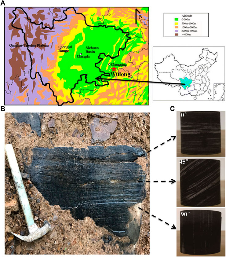
FIGURE 1. (A) Shale samples collected from Wulong, southeast of Sichuan Basin. (B) Silurian Longmaxi shale outcrops. (C) Cores are cut in three different directions.

TABLE 1

TABLE 1. Mineral composition of the Silurian Longmaxi shale sample (measured using an X-ray fluorescence spectrometer).

An ultrasonic pulse testing system is used to measure the velocities of P- and S-waves (SH-wave) in a shale sample. The measurements were carried out at room temperature and pressure, the main frequencies of P- and S-wave transducers were 1 and 0.5 MHz, respectively, and the test error was less than 1%. The measured velocities are shown in Table 2. The quantities $V_P\left(0^{\circ }\right)$ and $V_{SH}\left(0^{\circ }\right)$ represent the velocities of the P- and SH-waves along the normal to the bedding, respectively. The quantities $V_P\left({45}^{\circ }\right)$ and $V_{SH}\left({45}^{\circ }\right)$ represent the velocities of P- and S-waves at an angle of 45° to the bedding, respectively. The quantities $V_P\left({90}^{\circ }\right)$ and $V_{SH}\left({90}^{\circ }\right)$ represent the velocities of the P- and S-waves parallel to the bedding, respectively. It is seen that $V_P\left(0^{\circ }\right)<V_P\left({45}^{\circ }\right)<V_P\left({90}^{\circ }\right)$ and $V_{SH}\left(0^{\circ }\right)<V_{SH}\left({45}^{\circ }\right)<V_{SH}\left({90}^{\circ }\right)$. Thus, a shale sample has an equivalent VTI property and five independent elastic stiffness coefficients $C_{ij}$, which can be calculated using the measured velocity and density $\rho$ as (Wang, 2002; Mavko et al.,2003)

$\{\begin{array}{l}{c}_{11}=\rho V_P^{\mathrm{\hspace{0.17em}\hspace{0.17em}\hspace{0.17em}\hspace{0.17em}2}}\left({90}^{°}\right),c_{12}=c_{11}-2\rho V_{SH}^{\mathrm{\hspace{0.17em}\hspace{0.17em}\hspace{0.17em}\hspace{0.17em}\hspace{0.17em}\hspace{0.17em}\hspace{0.17em}\hspace{0.17em}2}}\left({90}^{°}\right),\\ c_{33}=\rho V_P^{\mathrm{\hspace{0.17em}\hspace{0.17em}\hspace{0.17em}\hspace{0.17em}2}}\left(0^{°}\right),c_{44}=\rho V_{SH}^{\mathrm{\hspace{0.17em}\hspace{0.17em}\hspace{0.17em}\hspace{0.17em}\hspace{0.17em}\hspace{0.17em}\hspace{0.17em}\hspace{0.17em}2}}\left(0^{°}\right),c_{66}=\frac{1}{2}\left(c_{11}-c_{12}\right),\\ c_{13}=-c_{44}+\sqrt{4{\rho }^2{V}_P^{\mathrm{\hspace{0.17em}\hspace{0.17em}\hspace{0.17em}\hspace{0.17em}4}}\left({45}^{°}\right)+\left(c_{11}+c_{44}\right)\left(c_{33}+c_{44}\right)-2\rho V_P^{\mathrm{\hspace{0.17em}\hspace{0.17em}\hspace{0.17em}\hspace{0.17em}2}}\left({45}^{°}\right)\left(c_{11}+c_{33}+2c_{44}\right)}.\end{array}(1)$

TABLE 2

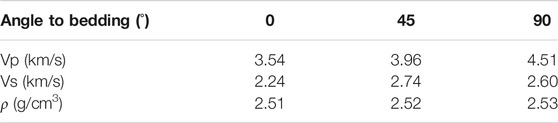
TABLE 2. Velocities of P- and S-waves measured in three directions.

The P-wave velocity as a function of angle is calculated using the following equation:

$V_P\left(\alpha \right)={\left(c_{11}{\sin }^2\alpha +c_{33}{\cos }^2\alpha +c_{44}+\sqrt{M}\right)}^{1/2}{\left(2\rho \right)}^{-1/2},(2)$

where $\alpha$ is the phase angle to the bedding normal and $M={[(c_{11}-c_{44}){\sin }^2\alpha -(c_{33}-c_{44}){\cos }^2\alpha ]}^2+{(c_{13}+c_{44})}^2{\sin }^{2}2\alpha$. The velocity of P-wave, which varies depending on the direction, is shown in Figure 2 and is used for further event-matching and location using data from the AE experiment (Figure 3). Since in subsequent AE experiments the sensors have only one component, only the P-wave velocity is used to locate events. The kinematics of P-wave in the TI medium weakly depends on the S-wave phase velocity (Alkhalifah, 1998; Jin and Stovas, 2018; Jin and Stovas, 2020). The magnitude of shale anisotropy can be represented by the P-wave velocity anisotropy parameter $\epsilon =(C_{11}-C_{33})/2C_{33}$ (Thomsen, 1986). The measured shale sample has strong P-wave anisotropy, since its ε is 0.27. The densities of the three samples are almost the same, and slight deviations can be caused by heterogeneity.

FIGURE 2

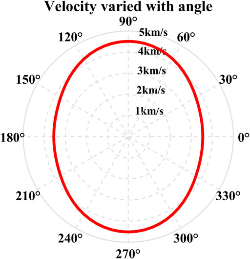
FIGURE 2. Variation of velocity with an angle to the axis of symmetry.

FIGURE 3

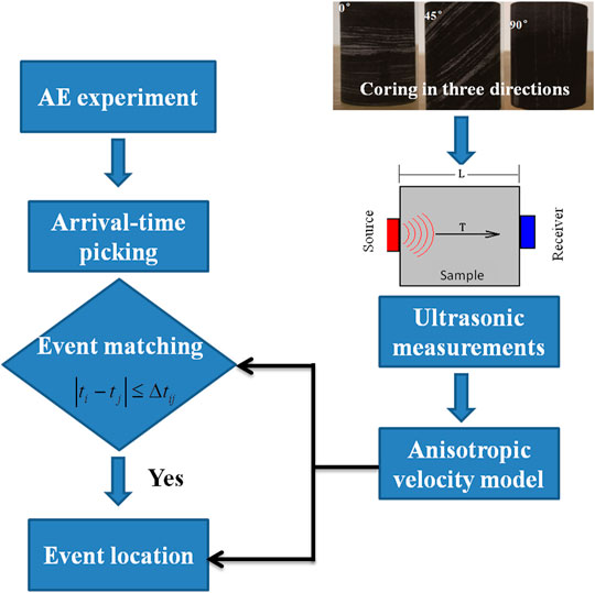
FIGURE 3. Workflow for events matching and location based on ultrasonic measurements and AE experiment.

3 Acoustic Emission Experiments

A three-point bend acoustic emission experiment is carried out on a semicylindrical shale sample that is 50 mm thick and has a radius of 50 mm (Figures 4A,B). The sample before fracturing did not contain natural fractures. Its axial direction is perpendicular to the bedding. Compressive loads are applied to three points with a ratio of 0.01 mm/min for 1 hour until the destruction of the sample. The AE signals are received by eight resonance-type sensors (SR150S) placed on the surface of the sample (Figure 4C). The sensors have a frequency range of 70∼280 kHz and a resonance frequency of 150 kHz. The main parameters of the AE experiment are shown in Table 3. The AE signal sampling frequency is 5,000 kHz with a sampling interval of 0.2 µs, a waveform threshold of 35 dB, a pre-sampling time of 150 µs, a sampling length of 4,000 points, and a total recording length of 800 μs for each acquisition segment. The eight AE sensors and 40-dB preamplifiers were used in the tests, and AE signals exceeding 40 dB were captured during fracturing. CT scans are performed before and after rock breakdown to determine fracture distribution. The results of the CT X-ray images are shown in Figures 4D,E. These results will be used as the true fracture distribution for comparing source locations.

FIGURE 4

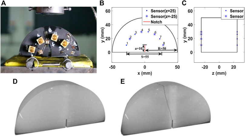
FIGURE 4. (A) Notched semicircular bend (NSCB) shale sample after unaxial loading. (B) The front view of sample geometry and eight AE sensors. The distance between the two supporting(S) is 55 mm and a 10mm notch is made in the middle of the lower part of the sample to cause a directed rupture. (C) The side view of sample geometry and four sensors are glued on the z = 25 mm plane (blue point) and the rest are on the z = −2 5mm plane(blue asterisk).X-ray images of CT scanning (D) and (E) after fracturing.

TABLE 3

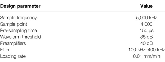
TABLE 3. Basic parameters of the AE experiment.

4 Event-Matching for Anisotropic Media

Event-matching aims to obtain AE signals from the same source event. It is carried out after the acquisition of the first arrivals (Figure 3). Ideally, an AE event is received and recorded by all eight sensors (Figure 5A). However, many AE events are received and recorded by only a few sensors (Figure 5B). This may be because these events are not strong enough to trigger all sensors for recording. To determine the location of the AE source, it is necessary to solve four unknown parameters, including the coordinates of the location (x₀, y₀, z₀) and the origin time (t₀). Therefore, valid AE signals are signals from the same source received by at least four sensors. Hence, reliable AE event-matching is crucial to locate the source.

FIGURE 5

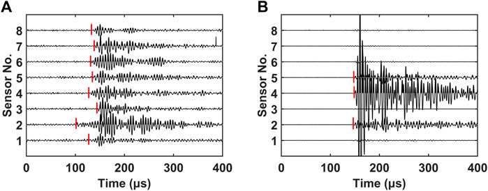
FIGURE 5. (A) AE event recorded by eight sensors. The red line represents the selected arrival times. (B) AE event received by only three sensors (Sensor 2, 4, and 5).

Event-matching can be achieved using a triangulation rule as shown in Figure 6. The difference between the AE arrival times from the two sensors is compared with the time threshold Δt to confirm if they are valid. The time threshold is usually constant and is expressed as the difference in travel time between the two farthest points or sensors in the sample (Feng et al., 2019). The arrival times of AE signals received by two sensors (t₁ and t₂) correspond to two sides of the triangle. Knowing the coordinates of two sensors, it is possible to calculate the travel time from one sensor to the other as a “third side” using a known velocity model. The signals can be identified as from the same source event, if the following matching condition is met:

$\left|t_1-t_2\right|\le \mathrm{\Delta }t.(3)$

FIGURE 6

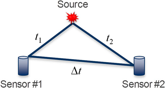
FIGURE 6. Principle of the triangulation method of event-matching.

In this three-point bending experiment, assuming the sample is isotropic, Δt is calculated as 30 μs using a constant velocity 3.54 km/s. As shown in Figure 7A, signals are received by four sensors, but the differences in arrival times between them are much greater than Δt, so this set of signals is recognized as invalid based on the formula Eq. 3. In this article, the Akaike information criterion (AIC) (Maeda, 1985) is used to determine the time of the first arrival of AE events. Although this method is convenient and highly effective, it can match redundant signals because received signals are mixed with boundary reflections or signals from other sources. As shown in Figures 7B,C, events No.4 and No.12 contain signals received by all eight sensors. If Δt is used as 30 µs, eight signals and six signals can be matched for events No.4 and No. 12, respectively, and thus both events are considered valid. However, neither of these two events can complete the subsequent location. Either the location result is outside the sample, or an unreliable solution is obtained. This is because redundant invalid events are matched as valid using a constant Δt, ignoring directional velocity variation.

FIGURE 7

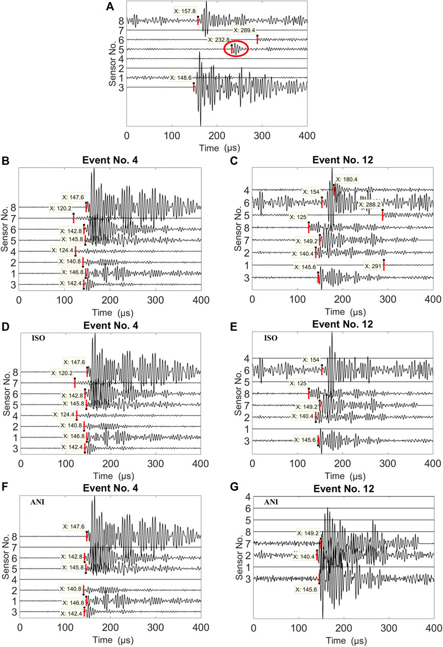
FIGURE 7. (A) Signals received by four sensors are considered invalid. Red lines represent first arrivals, and the red ellipse in the sensor 5 represents the boundary reflection. (B) Event No. 4 and (C) Event No. 12 received by all eight sensors before event-matching. (D) Event No. 4 and (E) Event No. 12 after event-matching using the constant Δt as 30 µs. (F) Event No. 4 and (G) Event No. 12 after event-matching using Δt calculated using anisotropic velocity.

To solve this problem, an improved matching condition is proposed, including the impact of anisotropy. In this AE experiment, sensors are arranged in a semicircle, and their angles are in a wide range (Figure 8A). As discussed in Eq. 2, the velocity of propagation of signals $V_p\left(\alpha \right)$ depends on the phase angle. Directional sines and cosines of the ith sensor relative to the jth sensor are respectively equal,

$\sin \alpha =\sqrt{{\left(x_i-x_j\right)}^2+{\left(y_i-y_j\right)}^2}/R_{ij}\mathrm{and }\cos \alpha =\left(z_i-z_j\right)/R_{ij},(4)$

where (x_i, y_i, z_i) and (x_j, y_j, z_j) are the coordinates of the ith and the jth sensor, respectively, and R_ij represents the linear distance between any of the two sensors. Figure 8B shows the calculated value of α of either of two sensors using Eq. 4. Figure 8C shows calculated $V_P\left(\alpha \right)$ using the formula Eq. 2 based on ultrasonic measurements. The time threshold Δt is now updated as

$\mathrm{\Delta }{t}_{ij}=R_{ij}/V_p\left(\alpha \right),(5)$

and the new matching condition is

$\left|t_i-t_j\right|\le \mathrm{\Delta }{t}_{ij}.(6)$

FIGURE 8

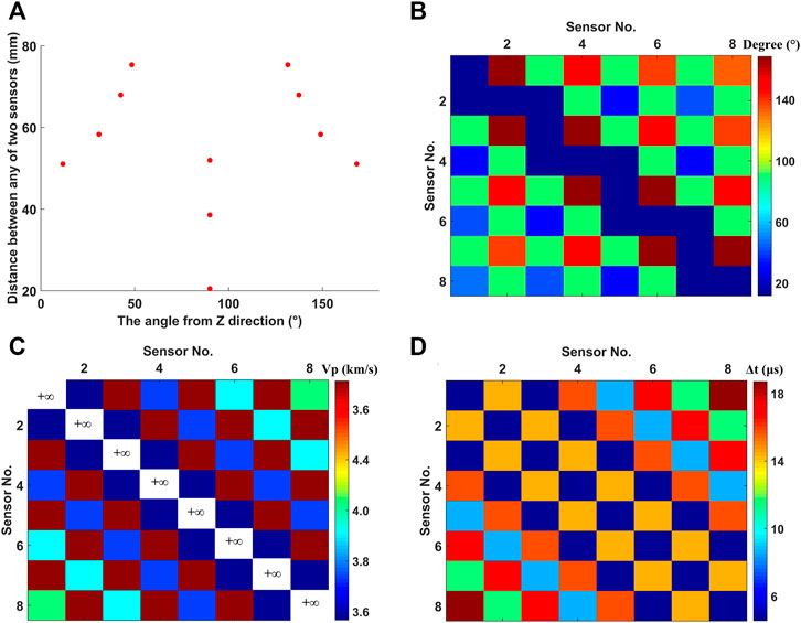
FIGURE 8. (A) Relationship between the distances between two sensors and the angle from the Z direction in a three-point bend experiment. (B) Directions between either of the two sensors. (C) Velocity variation between either of the two sensors. (D) Differences in travel time between either of the two sensors. It is noted that the time differences (Δt_ii) between the same sensors are equal to 0, and the propagation velocity is infinite.

The calculated value of Δt_ij between any of two sensors is shown in Figure 8D. The time differences between the two sensors range from 0 to 20 µs, which are less than the isotropic Δt (30 µs).

Compared to the initial results, using the improved matching condition that takes into account the impact of anisotropy, fewer signals are matched (Figures 7F,G). Six signals are matched for event No. 4, which is still recognized as a valid AE event, while only three signals are matched for event No. 12 and thus cannot be used for locating since the number of signals is less than four. In general, the results of anisotropic matching remove redundant events and thus reduce the total number of effective events (Figure 9A). A total of 179 valid events were obtained using event-matching without taking into account the anisotropy effect, and a total of 153 valid events are obtained using the new event-matching method taking into account velocity anisotropy. In particular, the number of events received by the four sensors is significantly reduced (Figure 9B). The reason is because that the anisotropic method uses a stricter threshold ($\Delta t$ has a lower value) than the isotropic method since the latter’s time threshold is calculated using a constant and relatively low velocity measured normal to the layer (0^o as shown in Figure 2), while the former’s time threshold calculated using higher velocity depending on the direction.

FIGURE 9

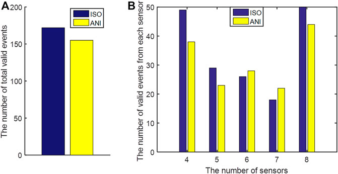
FIGURE 9. (A) Total number of valid events matched using isotropic (ISO) and anisotropic (ANI) methods. (B) Number of valid events from each sensor, matched using ISO and ANI event-matching methods.

5 Source Location Including Velocity Anisotropy

The source location can be determined by the source parameters inversion based on the known observational data. Source parameters, including coordinates and time of fracture initiation, can be estimated by resolving an inconsistent linear system (Geiger, 1912). As for an anisotropic medium, the function of the arrival time of the kth sensor $f_k$ is expressed as

$f_k\left(\mathbf{m}\right)=t+\frac{1}{V\left({\alpha }_k\right)}\sqrt{{\left(x_k-x\right)}^2+{\left(y_k-y\right)}^2+{\left(z_k-z\right)}^2},(7)$

where $\mathbf{m}={\left(t,x,y,z\right)}^T$ is the vector of the source parameters in terms of the origin time t and source coordinates (x, y, z) to be inverted, V (α_k) is the calculated velocity based on ultrasonic measurements, and α_k is the angle of the kth sensor to the Z axis (Figure 8A), which can be expressed as

$\sin {\alpha }_k=\sqrt{{\left(x_k-x\right)}^2+{\left(y_k-y\right)}^2}/l\mathrm{and}\cos {\alpha }_k=\left(z_k-z\right)/l,(8)$

where $l=\sqrt{{\left(x_k-x\right)}^2+{\left(y_k-y\right)}^2+{\left(z_k-z\right)}^2}$. Given a certain point ${\mathbf{m}}_{\mathbf{0}}={\left(t_0,x_0,y_0,z_0\right)}^T$_, $f_k\left(\mathbf{m}\right)$ can be expanded using the first-order Taylor series as

$f_k\left(\mathbf{m}\right)\approx f_k\left({\mathbf{m}}_{\mathrm{0}}\right)+\mathrm{A}\left(\mathbf{m-}{\mathbf{m}}_{\mathrm{0}}\right),(9)$

where $\mathrm{A}=\left[\begin{array}{cccc}\frac{\partial f_1}{\partial x}& \frac{\partial f_1}{\partial y}& \frac{\partial f_1}{\partial z}& \frac{\partial f_1}{\partial t}\\ ⋮& ⋮& ⋮& ⋮\\ \frac{\partial f_k}{\partial x}& \frac{\partial f_k}{\partial y}& \frac{\partial f_k}{\partial z}& \frac{\partial f_k}{\partial t}\end{array}\right]$. The source parameter update $\mathrm{\Delta }\mathbf{m}=\mathbf{m}-{\mathbf{m}}_0$ can be recovered as

$\Delta \mathbf{m}={\left({\mathbf{A}}^{\mathrm{T}}\mathbf{A}\right)}^{-1}{\mathbf{A}}^{\mathrm{T}}\mathrm{\Delta }{f}_k,(10)$

where $\mathrm{\Delta }{f}_k=f_k\left(\mathbf{m}\right)-f_k\left({\mathbf{m}}_{\mathrm{0}}\right)$, and k is greater than or equal to 4. The vector of the source parameters is solved iteratively using the formula Eq. 11 until the specified error criterion is met

${\mathbf{m}}_{n+1}={\mathbf{m}}_n+\mathrm{\Delta }{\mathbf{m}}_n,(11)$

where n stands for the number of iteration.

This method is applied to experimental AE data. We compare the location results using isotropic velocity and anisotropic velocity, as shown in Figures 10A,B. These results are also calibrated with the actual fracture distribution from CT scanning as shown in Figures 10C,D, in which the amplitude of source events is displayed using varied size of dots. The valid location results must satisfy in the spatial domain $-50mm\le x\le 50mm$, $0\le y\le 50mm$ and $-25mm\le z\le 25mm$. Although 179 events are matched using the isotropic condition, only 40 sources are located using the isotropic location method, in which 31 sources are within the valid spatial domain (Figures 10A,C); while for 153 events matched using the anisotropic condition, 99 sources are located using the anisotropic location method, in which 71 sources are inside the valid spatial domain (Figures 10B,D). The number of located sources using the isotropic method is much less than that using the anisotropic method. In addition, the located sources using anisotropic velocity are better aligned with the fracture distribution, and the strong source events (displayed with larger dots) are more focused on the starting position of the fractures. To further demonstrate the result, we show four results using different processes (Figures 10C–F): isotropic matching and isotropic location (ISO + ISO), anisotropic matching and anisotropic location (ANI + ANI), isotropic matching and anisotropic location (ISO + ANI), and anisotropic matching and isotropic location (ANI + ISO). The located sources of anisotropic matching and anisotropic location show the best agreement with the CT scanning results in terms of fracture distribution and starting position. Therefore, it is very important to take into account the influence of anisotropy on the velocity for both AE event location and event-matching. Although there are several sources of weak-amplitude located outside the semicircle sample (Figures 10B,D), this could be improved by more accurate arrival times selection and more receivers with wider geometry (receivers are placed only on planes Z = −25 mm and Z = 25 mm in this study).

FIGURE 10

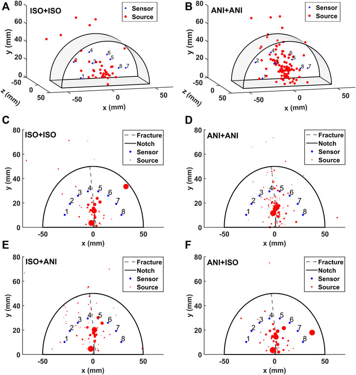
FIGURE 10. Source location results (3D display) using (A) an isotropic matching and isotropic location (ISO+ISO) method and (B) an anisotropic matching and anisotropic location (ANI+ANI) method. Comparison of fracture and location results (Front view) using (C) isotropic matching and isotropic location (ISO + ISO), (D) anisotropic matching and anisotropic location (ANI + ANI), (E) isotropic matching and anisotropic location (ISO + ANI), and (F) anisotropic matching and isotropic location (ANI + ISO). The gray dashed lines represent the fracture, and the magnitude of source events is displayed using dots of various sizes.

Finally, we analyze the located AE events at different stages of fracture, as shown in Figure 11. The first AE event is detected at 5800s after loading (Figure 11A). After a quiet period of about 10 min, several acoustic emission events occurred during the 6460–6500s period (Figure 11B). These events appear around the fracture, but their distribution does not follow the strike of the fracture. In the period of 6500–6600s (Figures 11C,D), a large number of acoustic emission events are detected that developed along the fracture.

FIGURE 11

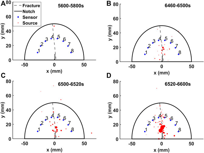
FIGURE 11. Located AE events at different fracturing times (A) 5600–5800s, (B) 6460–6500s, (C) 6500–6520s, (D) 6520–6600s.

6 Conclusion

Event-matching is a necessary process for pinpointing a location. Traditional methods of event-matching and location can be affected by velocity anisotropy, leading to further unreliable source location results. In the event-matching process, if velocity anisotropy is ignored, many redundant events or false AE events will be matched. Most of the source points detected by these false events are outside the sample, and the location results are incompatible with fracture distribution. In this article, we analyze the effect of anisotropy on the results of event-matching and location based on the three-point bend AE experiment. We achieve the event-matching and location taking into account the correction for anisotropic velocity, increasing the ratio of the number of detected sources to valid events, which may better help us in determining fracture characteristics. Real acoustic emission data applications show a clear improvement in location results over isotropic Geiger’s results. The location results are also calibrated by CT scanning results, which show good consistency and confirm the improvement in fracture characteristics. In fact, both the velocity model and the sensor geometry have a large impact on the location results. If the sensors are distributed over a wide range of directions, we must not only take into account the anisotropy of the velocity model but also consider the anisotropy of velocity in event-matching.

Data Availability Statement

The raw data supporting the conclusion of this article will be made available by the authors, without undue reservation.

Author Contributions

PW: acquisition and processing of AE data, data presentation, methodology, and original draft; FZ: the conception and design of the study, reviewing and editing, and supervision; X-YL: conceptualization, collected important background information, and manuscript editing.

Funding

This work was supported by the National Natural Science Foundation of China (U19B6003, 42122029) and the Strategic Cooperation Technology Projects of CNPC and CUPB (ZLZX2020-03).

Conflict of Interest

The authors declare that the research was conducted in the absence of any commercial or financial relationships that could be construed as a potential conflict of interest.

Publisher’s Note

All claims expressed in this article are solely those of the authors and do not necessarily represent those of their affiliated organizations, or those of the publisher, the editors, and the reviewers. Any product that may be evaluated in this article, or claim that may be made by its manufacturer, is not guaranteed or endorsed by the publisher.

References

Akram, J., and Eaton, D. W. (2016). A Review and Appraisal of Arrival-Time Picking Methods for Downhole Microseismic Data. Geophysics 81 (2), KS67–KS87. doi:10.1190/geo2014-0500.1

CrossRef Full Text | Google Scholar

Alkhalifah, T. (1998). Acoustic Approximations for Processing in Transversely Isotropic media. Geophysics 63 (2), 623–631. doi:10.1190/1.1444361

CrossRef Full Text | Google Scholar

Feng, X.-T., Young, R. P., Reyes-Montes, J. M., Aydan, Ö., Ishida, T., Liu, J.-P., et al. (2019). ISRM Suggested Method for In Situ Acoustic Emission Monitoring of the Fracturing Process in Rock Masses. Rock Mech. Rock Eng. 52 (5), 1395–1414. doi:10.1007/s00603-019-01774-z

CrossRef Full Text | Google Scholar

Ge, M. C. (2013). Analysis of Source Location Algorithms Part II: Iterative Methods. J. Acoust. Emission 21, 29–51.

Google Scholar

Geiger, L. (1912). Probability Method for the Determination of Earthquake Epicenters from the Arrival Time Only. Bull. St. Louis Univ. 8, 60–71.

Google Scholar

Gibbons, S. J., and Ringdal, F. (2006). The Detection of Low Magnitude Seismic Events Using Array-Based Waveform Correlation. Geophys. J. Int. 165 (1), 149–166. doi:10.1111/j.1365-246x.2006.02865.x

CrossRef Full Text | Google Scholar

Jin, S., and Stovas, A. (2020). S‐wave in 2D Acoustic Transversely Isotropic media with a Tilted Symmetry axis. Geophys. Prospecting 68 (2), 483–500. doi:10.1111/1365-2478.12856

CrossRef Full Text | Google Scholar

Jin, S., and Stovas, A. (2018). S‐wave Kinematics in Acoustic Transversely Isotropic media with a Vertical Symmetry axis. Geophys. Prospecting 66 (6), 1123–1137. doi:10.1111/1365-2478.12635

CrossRef Full Text | Google Scholar

King, A., and Talebi, S. (2007). Anisotropy Effects on Microseismic Event Location. Pure Appl. Geophys. 164 (11), 2141–2156. doi:10.1007/s00024-007-0266-8

CrossRef Full Text | Google Scholar

Li, J. H., and Qi, G. (2009). Improving Source Location Accuracy of Acoustic Emission in Complicated Structures. Journal of Nondestructive Evaluation 28, 1–8. doi:10.1007/s10921-009-0042-z

CrossRef Full Text | Google Scholar

Liu, Z., Zhang, F., and Li, X. (2019). Elastic Anisotropy and its Influencing Factors in Organic-Rich marine Shale of Southern China. Sci. China Earth Sci. 62, 1805–1818. doi:10.1007/s11430-019-9449-7

CrossRef Full Text | Google Scholar

Lonardelli, I., Wenk, H.-R., and Ren, Y. (2007). Preferred Orientation and Elastic Anisotropy in Shales. Geophysics 72, D33–D40. doi:10.1190/1.2435966

CrossRef Full Text | Google Scholar

López Comino, J. A., Heimann, S., Cesca, S., Milkereit, C., Dahm, T., and Zang, A. (2017). Automated Full Waveform Detection and Location Algorithm of Acoustic Emissions from Hydraulic Fracturing Experiment. Procedia Engineering 191, 697–702. doi:10.1016/j.proeng.2017.05.234

CrossRef Full Text | Google Scholar

Maeda, N. (1985). A Method for Reading and Checking Phase Time in Auto-Processing System of Seismic Wave Data. Jssj 38, 365–379. doi:10.4294/zisin1948.38.3_365

CrossRef Full Text | Google Scholar

Mavko, G., Mukerji, T., and Dvorkin, J. (2003). The Rock Physics Handbook-Tools for Seismic in Porous media. Cambridge University Press.

Google Scholar

Maxwell, S. C., Bennett, L., and Jones, M. (2010). Anisotropic Velocity Modeling for Microseismic Processing: Part 1—Impact of Velocity Model Uncertainty: SEG Technical Program Expanded Abstracts 2010. Denver,Colorado: Soc. Expl. Geophys., 2130–2134.

Google Scholar

Song, F., Kuleli, H. S., Toksöz, M. N., Ay, E., and Zhang, H. (2010). An Improved Method for Hydrofracture-Induced Microseismic Event Detection and Phase Picking. Geophysics 75 (6), A47–A52. doi:10.1190/1.3484716

CrossRef Full Text | Google Scholar

Thomsen, L. (1986). Weak Elastic Anisotropy. Geophysics 51 (10), 1954–1966. doi:10.1190/1.1442051

CrossRef Full Text | Google Scholar

Van Dok, R., Fuller, B., Engelbrecht, L., Sterling, M., and Hipoint, A. (2011). Seismic Anisotropy in Microseismic Event Location Analysis. The Leading Edge 30 (7), 766–770. doi:10.1190/1.3609091

CrossRef Full Text | Google Scholar

Vernik, L., and Nur, A. (1992). Ultrasonic Velocity and Anisotropy of Hydrocarbon Source Rocks. Geophysics 57 (5), 727–735. doi:10.1190/1.1443286

CrossRef Full Text | Google Scholar

Wang, Z. (2002). Seismic Anisotropy in Sedimentary Rocks, Part 1: A Single‐plug Laboratory Method. Geophysics 67 (5), 1415–1422. doi:10.1190/1.1512787

CrossRef Full Text | Google Scholar

Wuestefeld, A., Greve, S. M., Näsholm, S. P., and Oye, V. (2018). Benchmarking Earthquake Location Algorithms: A Synthetic Comparison. Geophysics 83 (4), KS35–KS47. doi:10.1190/geo2017-0317.1

CrossRef Full Text | Google Scholar

Zhang, F. (2019). A Modified Rock Physics Model of Overmature Organic-Rich Shale: Application to Anisotropy Parameter Prediction from Well Logs. J. Geophys. Eng. 16 (1), 92–104. doi:10.1093/jge/gxy008

CrossRef Full Text | Google Scholar

Zhang, F. (2017). Estimation of Anisotropy Parameters for Shales Based on an Improved Rock Physics Model, Part 2: Case Study. J. Geophys. Eng. 14, 238–254. doi:10.1088/1742-2140/aa5afa

CrossRef Full Text | Google Scholar

Zhang, F., Li, X.-y., and Qian, K. (2017). Estimation of Anisotropy Parameters for Shale Based on an Improved Rock Physics Model, Part 1: Theory. J. Geophys. Eng. 14, 143–158. doi:10.1088/1742-2140/14/1/143

CrossRef Full Text | Google Scholar

Zhang, H. L., Zhu, G. M., and Wang, Y. H. (2013). Automatic Microseismic Event Detection and Picking Method. Geophys. Geochemical Exploration 37 (2), 269–273.

Google Scholar

Zhou, Z. L., Zhou, J., Dong, L. J., Cai, X., Rui, Y. C., and Ke, C. T. (2017). Experimental Study on the Location of an Acoustic Emission Source Considering Refraction in Different media. Sci. Rep. 7 (1), 7472. doi:10.1038/s41598-017-07371-w

PubMed Abstract | CrossRef Full Text | Google Scholar