Phase-shift mode of the East Asian trough from December to February: Characteristic and possible mechanisms

Introduction

The East Asian trough (EAT) is a quasi-stationary planetary trough over East Asia in boreal winter, and its variation exerts a substantial influence on the local climate (Zou et al., 1991; Wang, 2007; Huang et al., 2012). Therefore, research on the EAT variation and the possible mechanism is of great significance.

From the monthly or seasonal mean aspect, a number of previous studies have demonstrated the factors contributing to the EAT variation. The atmospheric circulation factors include the Siberian High (Wu and Wang, 2002), Asian tropospheric polar vortex (Yu and Sun, 2021), West Pacific pattern (Linkin and Nigam, 2008; Takaya and Nakamura, 2013), Eurasian pattern (Wallace and Gutzler, 1981; Sung et al., 2009; Wang et al., 2019), and Arctic Oscillation (Gong et al., 2001; Wu and Wang, 2002; Wang et al., 2005; He et al., 2017), among others. The underlying surface factors include El Niño-Southern Oscillation (ENSO) (Zhang et al., 1996; Wang et al., 2000), western North Pacific Sea surface temperature (SST) anomalies (Sun et al., 2016; Lei et al., 2020), Arctic Sea ice (Wu et al., 1999; Wu and Zhang, 2010; Mori et al., 2014), snow cover (Chen and Sun, 2003; Luo and Wang, 2019), among others.

Previous studies have mainly investigated the monthly or seasonal mean EAT variation, while few studies have focused on the EAT’s month-to-month variations. Some case studies have shown that the EAT has a strong intermonthly phase shift. For example, in December 2005, the EAT was strong but weak in February 2006 (Park et al., 2008; Inaba and Kodera, 2010); in December 2015, the EAT was weak but strong in January 2016 (Song and Yuan, 2017). Such a phenomenon can hardly be explained by the analyses of seasonal mean or a single month, but it would challenge the prediction of the EAT and East Asian climate. Therefore, in this study, we attempt to answer the following two questions: (1) Is the phase shift an intrinsic mode of the EAT month-to-month variation in winter? (2) What is the possible mechanism responsible for the phase-shift mode of the EAT month-to-month variation? Addressing these two questions can deepen our understanding of the EAT variation, further providing a scientific basis for the prediction of the month-to-month variation in EAT and East Asian winter climate.

The remainder of this paper is organized as follows: Section of Data and Method introduces the datasets and methods. Section of Results demonstrates the phase-shift mode of the EAT month-to-month variation in December-January-February and the possible mechanism. Finally, some discussions and a summary are given.

Data and method

Monthly and daily mean atmospheric reanalysis data (1979–2019) are from the European Centre for Medium-Range Weather Forecasts (ECMWF) ERA5 reanalysis (Hersbach et al., 2020). The analyzed variables include the three-dimensional winds, geopotential height, and air temperature. The horizontal resolution of the ERA5 reanalysis is 1.0°×1.0° longitude by latitude. Monthly sea ice data (1870–2019) are from the United Kingdom. Meteorological Office Hadley Centre Global Sea Ice and Sea Surface Temperature dataset (Rayner et al., 2003) and have a horizontal resolution of 1.0°×1.0° longitude by latitude. Monthly land surface air temperature data (v4.04) (1901–2019) are from the Climate Research Unit (CRU) (Harris et al., 2020) and have a horizontal resolution of 0.5°×0.5° longitude by latitude. The monthly latent and sensible heat flux (1958–2019) are from the Woods Hole Oceanographic Institution Objectively Analyzed air-sea Fluxes (OAFlux) object (Yu et al., 2008) and have a horizontal resolution of 1.0°×1.0°. Monthly global ocean heat content data (1940–2019) are from the Institute of Atmospheric Physics, Chinese Academy of Science (Cheng and Zhu, 2016) and have a horizontal resolution of 1.0°×1.0°.

The analysis period in this study is from January 1979 to December 2019, which is the common period of the aforementioned data. All monthly data are subtracted by their calendar monthly mean to obtain anomalies, and their long-term trends are subsequently removed. A two-tailed Student’s t test is used to estimate the statistical significance of the correlation and composite analyses. winter is defined as the mean of December, January, and February. For example, the winter of 1980 indicates the period from December 1979 to February 1980. The key region used to define the winter EAT is over 25°-50°N, 110°-150°E, similar to a previous study (Wang and He, 2012).

The extended empirical orthogonal function (EEOF) is an objective method to distinguish modes for a compound of multiple variables (Wang, 1992). By applying one climatic variable in sequential time, the method can separate the variable’s temporal-dependent modes (e.g., Wang and An, 2005). According to the EEOF method, three anomalous monthly fields (December, January, and February) are used to construct the matrix in this study. The monthly fields share the same time series for each principal component of the EEOF mode. The rule of North et al. (1982) is used to evaluate the eigenvalue separation.

The horizontal component of wave activity fluxes is calculated according to Takaya and Nakamura (2001). The synoptic components are separated by applying a 2–10-day Lanczos bandpass filter on daily data with 21 weights. The storm track is estimated by the standard deviation of 2–10-day bandpass filtered 300 hPa geopotential height (Lee et al., 2012; Chen et al., 2015). The geopotential height tendency caused by synoptic eddies is estimated by the equation (Lau and Holopainen, 1984; Lee et al., 2012): $\frac{\partial \mathrm{Z}}{\partial \mathrm{t}}={\nabla }^{-2}\left[-\frac{f}{g}\overline{\nabla \left(V^{\prime }{\zeta }^{\prime }\right)}\right]$, where f is the Coriolis parameter, g is the acceleration of gravity, V is the horizontal wind, and $\zeta$ is the relative vorticity. The operator ${\nabla }^{-2}$ represents the inverse Laplace transformation. The overbar and prime represent the monthly mean and synoptic component, respectively.

Results

Phase-shift mode of the EAT month-to-month variation

The EEOF analysis is performed on the 500 hPa geopotential height anomalies over the EAT key region from December to the following February. Three EEOF modes could be distinctly separated based on the rule of North (North et al., 1982), among which the second EEOF (EEOF2) mode presents a phase shift of the EAT month-to-month variations from December to February (Figure 1A). The pattern in Figure 1A is regarded as positive EEOF2 in this study. The positive/negative EEOF2 indicates that the EAT is weakened/strengthened in December but shifts to the opposite phase in the following February. EEOF2 explains approximately 21.1% of the total variance in the EAT month-to-month variability. The EEOF2 principal component time series (PC2) is shown in Figure 1B. It exhibits noticeable interannual variability.

FIGURE 1

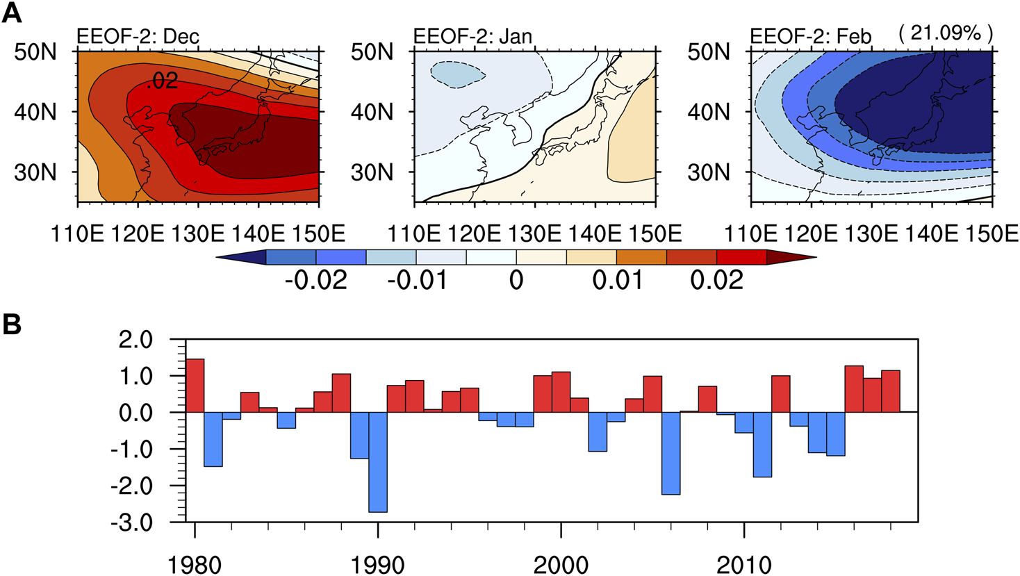
FIGURE 1. (A) Spatial pattern for EEOF2 of the monthly 500 hPa geopotential height anomalies over East Asia in December (top-left), January (top-middle), and February (top-right). The corresponding standardized PC2 is shown in (B).

To further examine the capacity of EEOF2 in describing the EAT month-to-month variations in winter, the relationship between EEOF2 and the EAT index is investigated. The EAT index is defined as the standardized area-averaged 500 hPa geopotential height anomalies over the corresponding key region. The correlation coefficients of PC2 with the EAT index in December, January, and February are 0.62, -0.05, and -0.67, respectively. The correlation coefficients in December and February are significant at the 95% confidence level. Furthermore, the EAT indices during the three winter months are calculated during anomalous positive and negative EEOF2 years. An anomalous positive (negative) EEOF2 year is selected when the standardized PC2 index is greater than 0.75 (less than -0.75), and the absolute PC2 index is greater than the absolute principal component time series of EEOF1 and EEOF3. Therefore, EEOF2 acts as the dominant mode of the EAT month-to-month variation during the anomalous EEOF2 years. The monthly EAT indices in these anomalous EEOF2 years are shown in Figure 2. In all positive EEOF2 years, the EAT is weakened in December but strengthened in February (Figure 2A). The situations are opposite in most negative EEOF2 years (except for 1990) (Figure 2B). The 1990 winter had a slightly weakened EAT in December, opposite to that of negative EEOF2. This is probably because the monthly EAT anomaly is contributed by all the intrinsic modes of the EAT month-to-month variation in winter, while EEOF2 is just one of these modes. Therefore, in some cases, it is rational to observe the inconsistent EAT anomaly in a specific month relative to the corresponding EEOF2 pattern. Overall, EEOF2 can reflect the phase shift of the EAT month-to-month variation in winter.

FIGURE 2

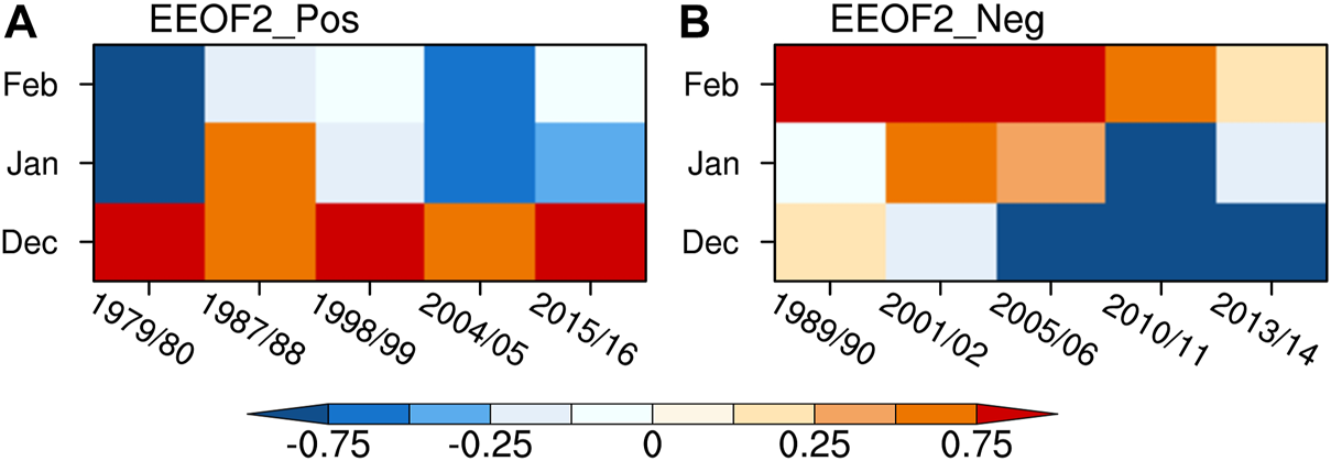
FIGURE 2. (A) The standardized winter monthly EAT indices during the years with the positive phase of the EEOF2. (B) Same as in (A) but during the years with the negative phase of EEOF2.

Previous studies indicated that the EAT has a profound impact on East Asian winter air temperature (e.g., Wang, 2007). The phase-shift mode of the EAT during the winter months could lead to reverse temperature anomalies in December and February. As shown in Figure 3A, in December, the positive EEOF2 is associated with a weakened EAT, which could significantly depress the climatological northerly wind and result in warm temperature anomalies over East Asia. January is the transient period during the anomalous EEOF2 years, and the atmospheric circulation and temperature anomalies are consequently weak in this month (Figure 3B). In February, the positive EEOF2 is associated with the strengthened EAT, enhancing the climatological northerly wind and causing cold temperature anomalies over East Asia (Figure 3C). Such a result is consistent with the previously reported warm early winter and cold late winter (or vice versa) (Inaba and Kodera, 2010; Song and Yuan, 2017), indicating that the EAT phase-shift mode plays an important role in the month-to-month variations in the East Asian winter air temperature.

FIGURE 3

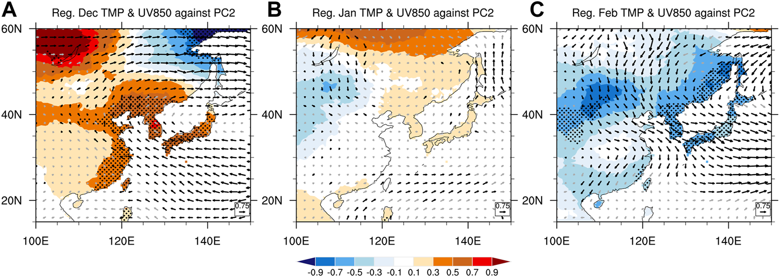
FIGURE 3. Regressed CRU air temperature anomalies (color; unit: °C) and 850 hPa horizontal wind anomalies (vector; unit: m/s) against PC2 in (A) December during 1979–2018 and (B) January and (C) February during 1980–2019. The anomalies significant at the 95% confidence level are shaded by dots. Black vectors are significant at the 95% confidence level.

Possible mechanisms responsible for the EAT phase-shift mode

To explore the possible mechanism responsible for the EAT phase-shift mode, we first investigate the EEOF2-related atmospheric circulation anomalies. Corresponding to the positive EEOF2, the significant positive 500 hPa geopotential height anomalies are over the EAT key region in December (Figure 4A), indicating the significant weakness of the EAT. In addition, a significant dipole pattern of 500 hPa geopotential height anomalies could be observed over the North Atlantic. The positive and negative centers of the dipole pattern are located over the midlatitude North Atlantic and Greenland, respectively, resembling the positive NAO (Wallace and Gutzler, 1981). Over the Eurasian continent, there is a Rossby wave train, which could connect the NAO and EAT. In January, the atmospheric circulation anomalies related to EEOF2 are relatively weak (Figure 4B). In February, corresponding to the positive EEOF2, there are significant negative geopotential heights over the EAT key region, indicating the enhanced EAT (Figure 4C). There is also a wave train over the Eurasian continent propagating eastward, with an anomalous anticyclone over the polar region, indicating that the Arctic climate anomalies could be related to the EEOF2 in February.

FIGURE 4

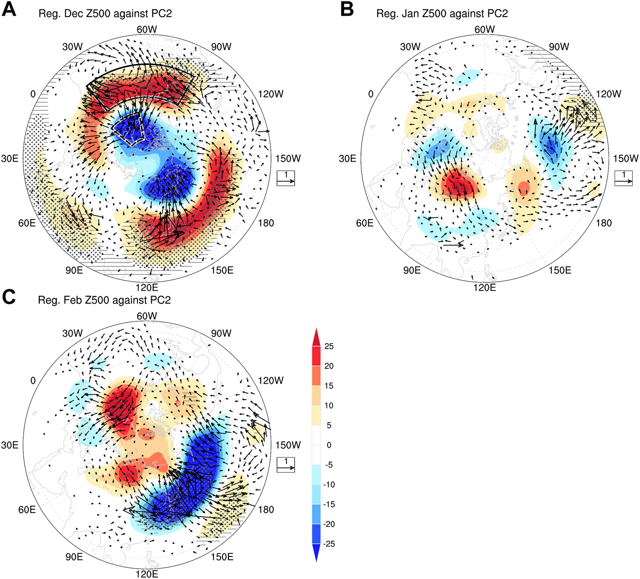
FIGURE 4. Regressed 500 hPa geopotential height anomalies (color; unit: m) against PC2 and the associated 300 hPa wave activity fluxes (vector; unit: m²/s²) in (A) December during 1979–2018 and (B) January and (C) February during 1980–2019. The hatched (dotted) areas are significant at the 95% (99%) confidence level. Vectors less than 0.1 m²/s² are not shown.

The above analyses illustrate a close relationship between the EEOF2 and December NAO. To further understand the connection between the December NAO and EEOF2, an NAO index is defined as the standardized difference between the area-average 500 hPa geopotential height anomalies over the regions of 25°–45°N, 90°-20°W, and 55°-75°N, 50°-10°W (boxes in Figure 4A). We also calculate the NAO index by applying the EOF analysis to the 500 hPa geopotential height anomalies over the region of 25°–90°N, 80°W-20°E, similar to previous studies (Davini and Cagnazzo, 2014; Oshika et al., 2015). The two NAO indices are highly correlated, with a coefficient of 0.95 in December. This result indicates that the NAO defined in this study is reasonable. The scatterplot between PC2 and the December NAO index is shown in Figure 5. The correlation coefficient between PC2 and the December NAO index is 0.50, significant at the 95% confidence level, indicating the close connection between the two factors. Generally, the positive (negative) December NAO could cause the positive (negative) EEOF2 in winter. The analysis of the same sign ratio shows that, in 80% of anomalous EEOF2 years, EEOF2 and the December NAO are in phase, and the corresponding absolute NAO indices are greater than 0.5. Therefore, the December NAO could be an important factor influencing EEOF2.

FIGURE 5

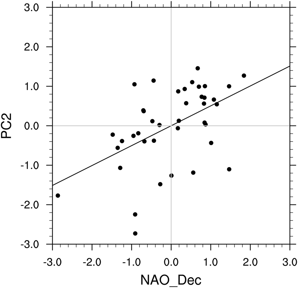
FIGURE 5. Scatterplot of the December NAO index and PC2. The line indicates the linear regression of PC2 against the December NAO index.

Figure 6 shows the December NAO-related simultaneous and lagged atmospheric circulation anomalies. This suggests that in December, the positive NAO triggers the Rossby wave train over midlatitude Eurasia, leading to a significantly weakened EAT (Figure 6A). In January, the NAO pattern still exists but is significantly weakened compared to December. At this time, the NAO-triggered Rossby wave train propagates eastward over high-latitude Eurasia, leading to a significant anomalous anticyclone around the Kara Sea; however, the atmospheric responses over East Asia are pretty weak (Figure 6B). In February, the NAO signal almost disappears while a wave train propagates from the Kara Sea to East Asia, significantly strengthening the EAT (Figure 6C).

FIGURE 6

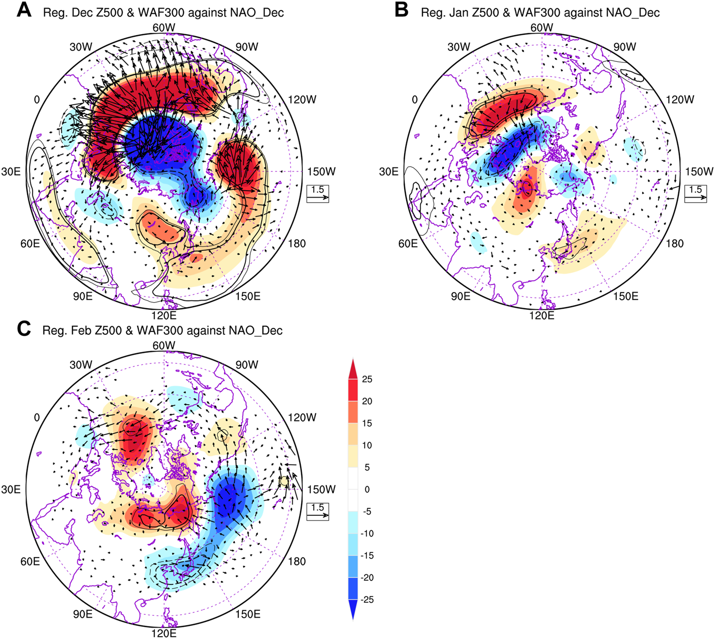
FIGURE 6. Regressed 500 hPa geopotential height anomalies (color; unit: m) against the December NAO index and the associated 300 hPa wave activity fluxes (vector; unit: m²/s²) in (A) December during 1979–2018 and (B) January and (C) February during 1980–2019. The positive/negative anomalies significant at the 90 and 95% confidence levels are enclosed with thin and thick solid/dashed contours. Vectors less than 0.1 m²/s² are not shown.

Figure 6C also raises a question: how does the preceding December NAO lead to atmospheric circulation anomalies around the Kara Sea in February when the NAO signal disappears? Previous studies have reported that Arctic Sea ice could be a medium for memorizing preceding climate signals (e.g., Wu et al., 2011; Cohen et al., 2014). Therefore, the relationship between the Arctic Sea ice anomalies and the December NAO is analyzed. Figure 7 suggests that the December NAO has a close relationship with the Baffin Bay Sea ice and a gradually intensified linkage with the Barents-Kara (BK) Sea ice from December to February. In addition, the February EAT-related Arctic Sea ice anomalies are only located over the BK Sea (Figure not shown). Therefore, we focus on the role of the BK Sea ice anomalies. The sign reversed area-average sea ice concentration anomalies over the region of 67.5°–80.5°N, 30.5°-75.5°E (box in Figure 7C) are used to measure the sea ice variability over the BK Sea, marked as the BKSIC index. Correlation analysis also indicates an increase in the correlations of December NAO with the January and February BKSIC from 0.33 to 0.46 (both are significant at the 95% confidence level).

FIGURE 7

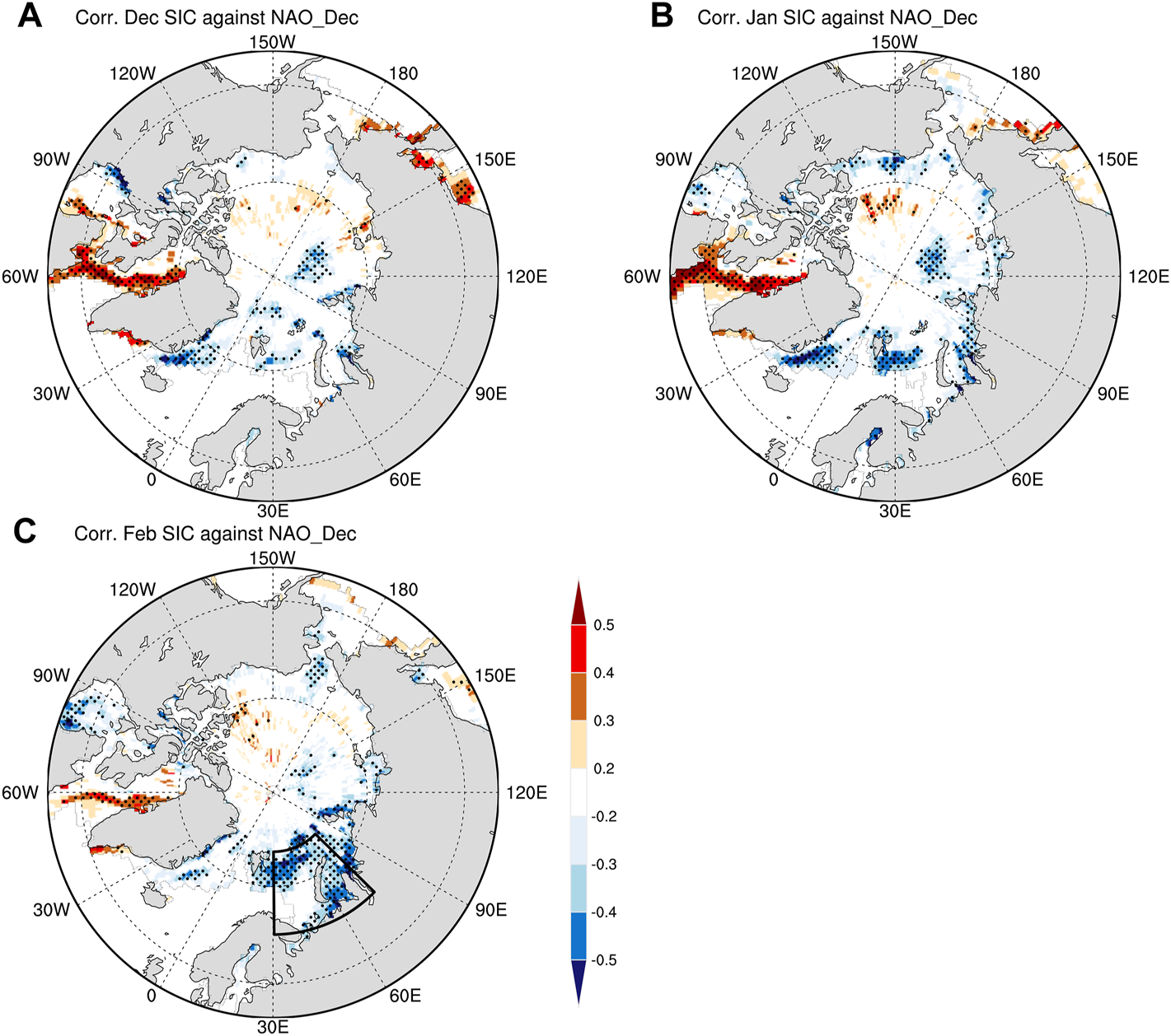
FIGURE 7. Correlation coefficients between the December NAO index and the Arctic Sea ice anomalies in (A) December during 1979–2018 and (B) January and (C) February during 1980–2019. The anomalies significant at the 90% confidence level are shaded by dots.

We further analyze the December NAO-related atmospheric and oceanic conditions to explore the physical processes for the NAO’s influence on the BK Sea ice. Generally, the positive feedback between the NAO and the underlying diabatic forcing favors maintaining the NAO with an equivalent barotropic structure (DeWeaver and Nigam, 2000; Pan, 2005; Ren et al., 2009). The regressed meridional temperature gradient and 300 hPa zonal wind anomalies over the North Atlantic against the December NAO index are shown in Figure 8. Concurrent with the positive NAO in December, there are negative (positive) temperature gradient anomalies at approximately 52.5°N (32.5°N) over the North Atlantic (Figure 8A), causing the acceleration (deceleration) of the north (south) part of the North Atlantic westerly jet stream (Figure 8B) according to the thermal wind theory. Subsequently, the North Atlantic storm track presents a northward displacement (Figure 9A). Accompanied by the strengthened storm track approximately 60°N over the North Atlantic, the synoptic eddy forcing causes significant negative geopotential height tendencies over Greenland and positive ones over the midlatitude North Atlantic (Figure 9B), favoring the maintenance of the positive NAO with an equivalent barotropic structure. The effects of synoptic eddy forcing are similar to those in previous studies (Lau and Holopainen, 1984; Lee et al., 2012). At the low-level troposphere, an anomalous anticyclone is over the midlatitude North Atlantic, and an anomalous cyclone is around Iceland (Figure 10A). The BK Sea is over the east flank of the Icelandic Low, and the anomalous southerly wind dominates this region, leading to significant warm air temperature anomalies over northern Europe and the BK Sea (Figure 10A). However, at this time, the oceanic near-surface layer temperature anomalies (weighted vertical average at the depths of 1, 5, and 10 m) in the Barents Sea are insignificant (Figure 10B), and the response of sea ice will be weak (Figure 7A). Due to the average sea ice thickness in the BK Sea being no more than 5 m (King et al., 2017; Kwok, 2018), we consider the oceanic temperature at 1–10 m to reflect the oceanic near-surface layer’s thermal conditions even with the sea ice cover.

FIGURE 8

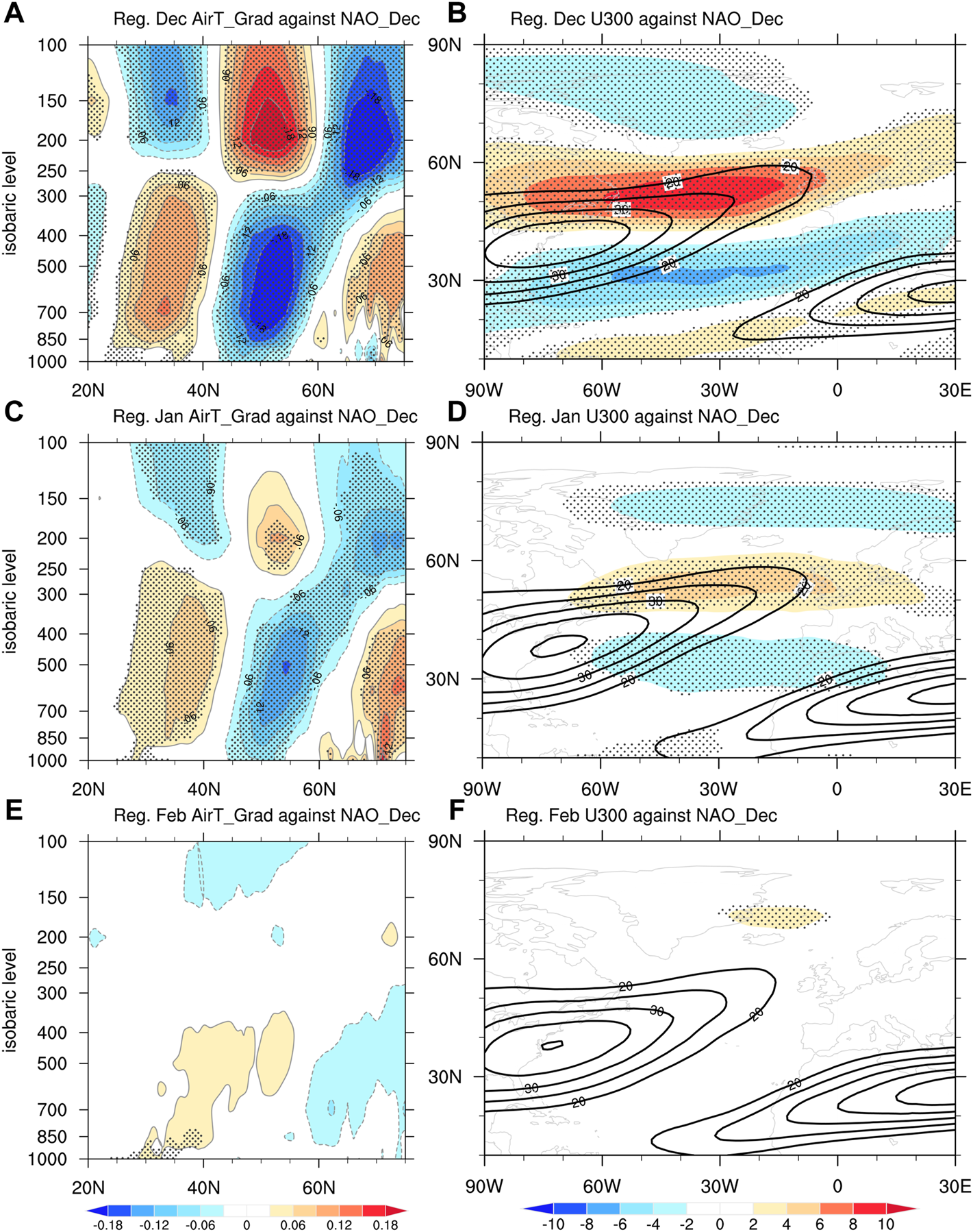
FIGURE 8. (A) Latitude-pressure cross-section of the regressed meridional temperature gradient averaged along 50°W-10°W against the December NAO index in December during 1979–2018 (color; unit: °C/lat-degree). (B) Regressed 300 hPa zonal wind anomalies (color; unit: °C) against the December NAO index in December during 1979–2018. (C,D) Same as in (A,B) but in January during 1980–2019. (E,F) Same as in (A,B) but in February during 1980–2019. The anomalies significant at the 90% confidence level are shaded by dots. The contours in (B,D,F) depict the climatology of the 300 hPa zonal wind.

FIGURE 9

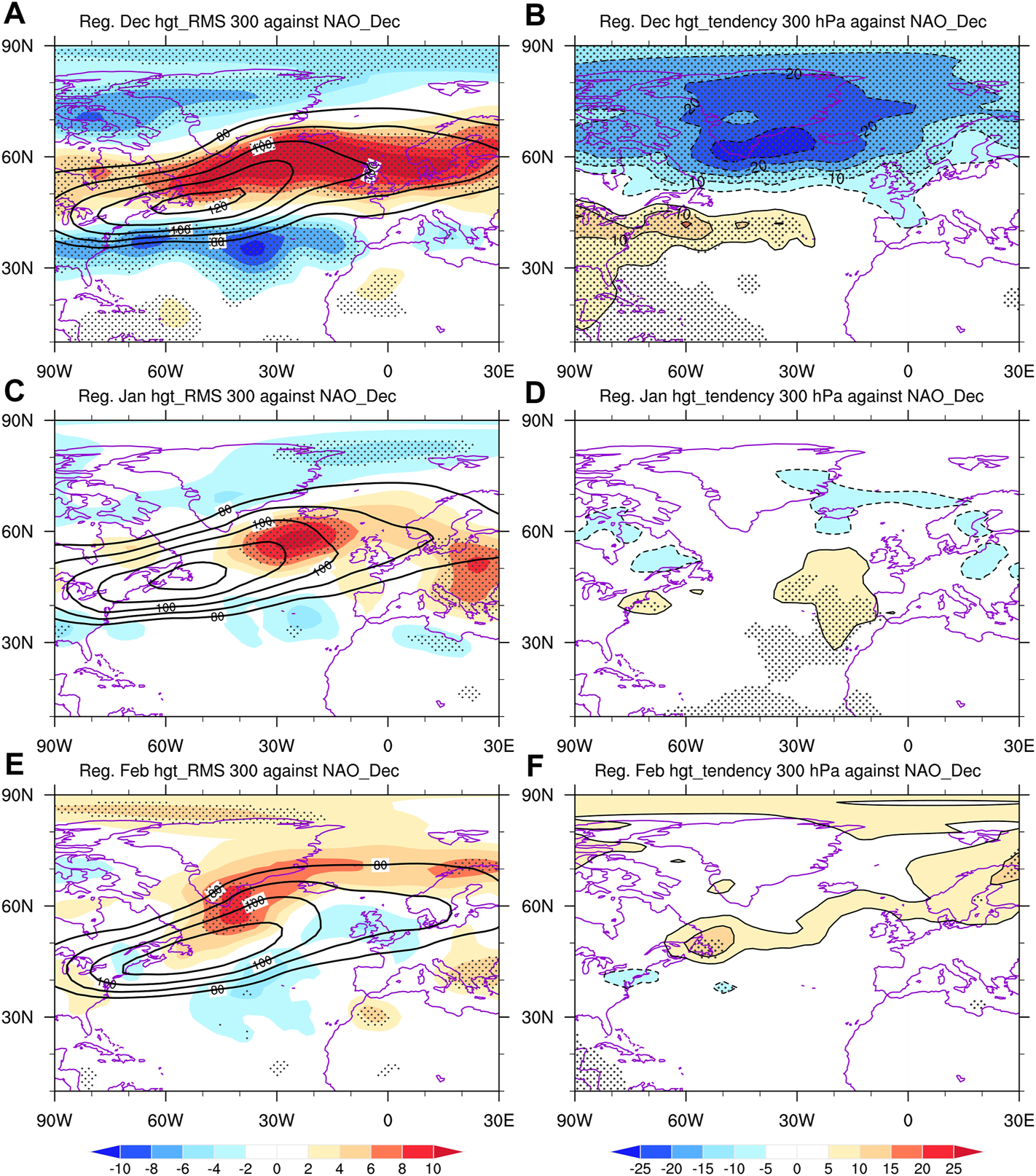
FIGURE 9. Regressed (A) 300 hPa storm track anomalies (color; unit: m), and (B) 300 hPa geopotential height tendency induced by the synoptic eddies (color; unit: m/day) against the December NAO index in December during 1979–2018. (C,D) Same as in (A,B) but in January during 1980–2019. (E,F) Same as in (A,B) but in February during 1980–2019. The anomalies significant at the 90% confidence level are shaded by dots. The contours in (A,C,E) depict the climatology of the 300 hPa storm track.

FIGURE 10

FIGURE 10. Regressed (A) 2 m air temperature anomalies (color; unit: °C) and 850 hPa horizontal wind anomalies (vector; unit: m/s), (B) weighted vertical average oceanic temperature (color; unit: °C) at the 1–10 m depth against the December NAO index in December during 1979–2018. (C,D) Same as in (A,B) but in January during 1980–2019. (E,F) Same as in (A,B) but in February during 1980–2019. The anomalies significant at the 90% confidence level are shaded by dots. Black vectors in (A,C,E) are significant at the 90% confidence level.

In January, the meridional temperature gradient anomalies with respect to the positive December NAO move northward and become weak (Figure 8C), as do the 300 hPa zonal wind anomalies over the North Atlantic (Figure 8D) and North Atlantic storm track (Figure 9C). The above process causes positive geopotential height tendencies around Iceland and negative ones around the Azores Islands (Figure 9D). The synoptic eddy forcing favors the northeastward displacement of the positive NAO but is relatively weaker in January than in December. Although the NAO signal becomes weak, the resultant anomalous cyclone is still over the high-latitude North Atlantic (Figure 10C). Significantly anomalous southerlies still prevail over northern Europe and the BK Sea, warming the regions. Under the continuous influence of the atmosphere from December to January, the warm temperature anomalies in the oceanic near-surface layer become stronger and more significant over the Barents Sea (Figure 10D). The anomalous warming air and oceanic temperature would be unfavorable to ocean freeze-up; therefore, significant BK Sea ice reduction can be observed (Figure 7B).

In February, the meridional temperature gradient and mean flow change insignificantly (Figures 8E,F), and no significant synoptic feedbacks are generated (Figures 9E,F). Such a situation hardly contributes to the NAO pattern maintenance. The December NAO-related atmospheric circulation anomalies are very weak over the North Atlantic (Figure 10E). In contrast, because of the intrinsic feature of the oceanic anomalies with a slow variation, significant oceanic temperature anomalies still exist over the BK Sea, and almost all the temperature anomalies over the BK Sea are greater than 0 °C (Figure 10F). The environment is still unfavorable for the regional sea ice formation; therefore, the BK sea ice significantly decreases in February (Figure 7C), although the NAO signal disappears. Associated with the less-than-normal BK Sea ice is a noticeable anticyclone over the BK Sea (Figure 11A), which is consistent with previous studies (e.g., Wu et al., 2011; Mori et al., 2014). Besides the local impacts, the less-than-normal BK Sea ice could trigger a Rossby wave train, leading to the significantly strengthened EAT in February (Figure 11A). Moreover, we also examine the February atmospheric circulation anomalies related to the January BK Sea ice anomalies (Figure 11B). The results are similar to those linked to the February BK Sea ice anomalies (Figure 11A), although the corresponding intensity and significance are somewhat weak. The January BK Sea ice status could provide prediction information for the local sea ice and EAT anomalies in February. Accordingly, with the BK Sea ice as a bridge, the December NAO significantly influences the following February EAT and contributes to the EEOF2 formation.

FIGURE 11

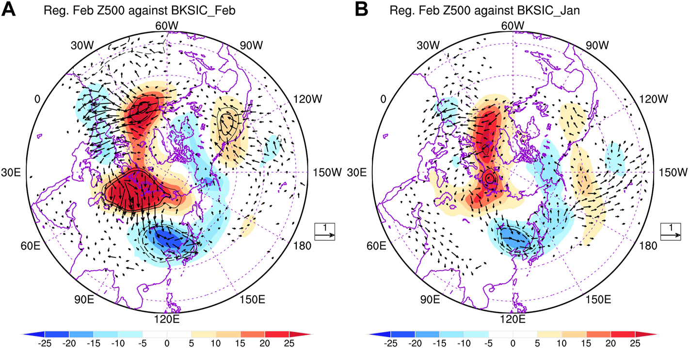
FIGURE 11. (A) Regressed 500 hPa geopotential height anomalies (color; unit: m) against the February BKSIC index and the associated 300 hPa wave activity fluxes (vector; unit: m²/s²) in February during 1980–2019. (B) Same as in (A) but for the results regressed against the January BKSIC index. The positive/negative anomalies significant at the 90 and 95% confidence levels are enclosed with thin and thick solid/dashed contours. Vectors less than 0.1 m²/s² are not shown.

Discussion and conclusion

Discussion

In this study, we have demonstrated that the December NAO could contribute to the phase shift of the EAT month-to-month variation in winter through the resultant BK Sea ice anomalies. Although the 1990 winter is a distinct case among the typical negative EEOF2 pattern years, we can also observe a strongly negative NAO with an index of -0.86 in December. However, the strongly negative NAO was concurrent with a slightly weakened EAT, opposite to the general influence of the negative NAO on the simultaneous EAT. The reason is probably that the NAO is only one of the various factors impacting the EAT; therefore, the solo NAO cannot sufficiently explain the monthly EAT anomaly in some cases. Consistent with the proposed mechanism, following the negative NAO in December, the BK Sea ice was more than normal in February, with an index of 0.95 in the 1990 winter. Subsequently, the more-than-normal BK Sea ice could weaken the simultaneous EAT (Figure 2B).

The December NAO is an important factor for EEOF2. It is crucial to know why the NAO pattern is formed in December. To answer this question, we investigate the air-sea interactions over the North Atlantic in November and December. Prior to the positive NAO in December, a dipole pattern of the 500 hPa geopotential height anomalies resembling the positive NAO, has been established in November (Figure 12A). With the equivalent barotropic structure, the atmospheric circulation anomalies in November could decrease (increase) the climatological zonal wind in the latitude belt of 30°–40°N (20°-30°N and 50°-60°N) over the North Atlantic (Figure 12C). The decreased (increased) climatological zonal wind would depress (enhance) the regional evaporation, reduces (intensifies) the heat loss from the ocean, and then tends to warm up (cool down) the ocean. Concurrently, there is a triple pattern of the SST anomalies over the North Atlantic in November (Figure 12E). Such a pattern could be maintained and intensified by the above-mentioned atmospheric forcing. In turn, the underlying SST could probably influence the middle tropospheric thickness (difference between the 500 hPa and 1,000 hPa geopotential height) and then favors maintaining the above atmospheric circulation anomalies (Figure 12G). With the positive feedback in the air-sea interaction over the North Atlantic, the atmospheric circulation and SST anomalies could persist into December, and the NAO and triple SST patterns are well formed in December (Figures 12B,F). In addition, the local air-sea interaction (Figures 12D,H) would favor maintaining the NAO and SST anomalies in December. These physical processes are also similar to previous studies (e.g., Peng et al., 2003; Pan, 2005).

FIGURE 12

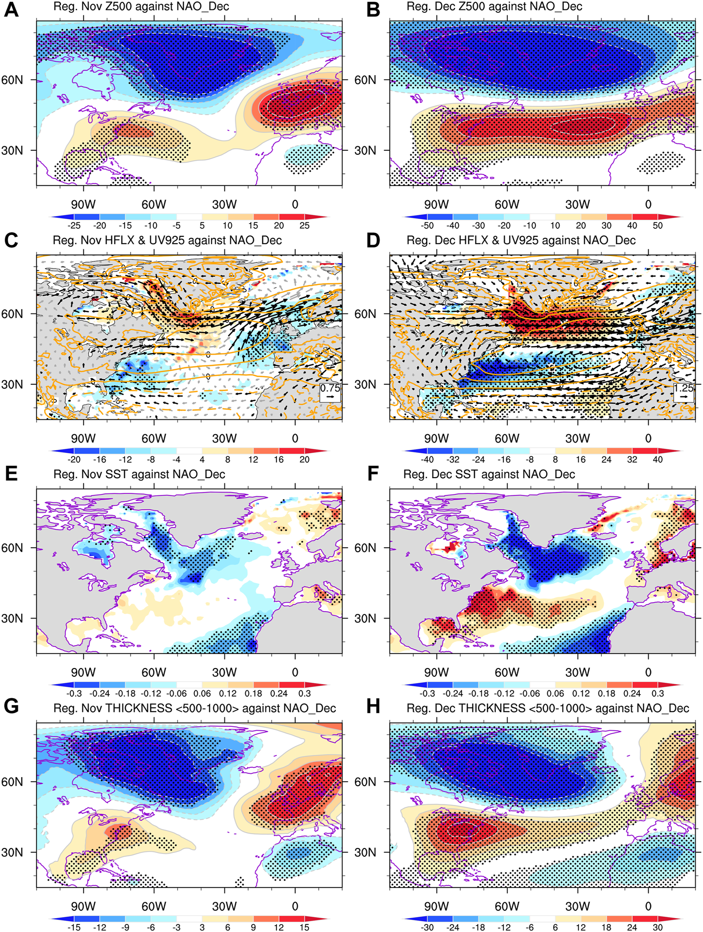
FIGURE 12. Regressed (A) November and (B) December 500 hPa geopotential height anomalies (unit: m) against the December NAO index during 1979–2018. (C,D) Same as in (A,B) but for the regressed turbulent heat flux anomalies (color; unit: W/m²) and 925 hPa horizontal wind anomalies (vector; unit: m/s). The turbulent heat flux is the sum of the sensible and latent heat flux, with the positive directed upward. The orange contours indicate the climatology of the 925 hPa zonal wind for the corresponding month during 1979–2018. (E,F) Same as in (A,B) but for the regressed SST anomalies (unit: °C). (G,H) Same as in (A,B) but for the regressed middle tropospheric thickness anomalies (unit: m). The anomalies significant at the 90% confidence level are shaded by dots. Black vectors in (C,D) are significant at the 90% confidence level.

On the other hand, the December NAO is probably not the ultimate factor influencing EEOF2. For example, the winter of 1988 was accompanied by a positive EEOF2 but with the December NAO index less than -1.0; the negative EEOF2 was in the winter of 2014 but with the December NAO index greater than 1.4. In the two cases, the positive/negative EEOF2 was well formed but with the strongly out-phase December NAO. Such results imply that there are probably other factors influencing EEOF2. As reported in a previous study, the super El Niño events can lead to the warm-cold transition over East Asia from December to January (Geng et al., 2017). In addition, the central Pacific ENSO could cause the phase shift of the surface air temperature anomalies in China from December to January during the post-1997 period (Li et al., 2021). Moreover, Xu et al. (2022) have illustrated the phase shift of the Eurasian surface air temperature anomalies from December to January-February. They have also demonstrated the possible contribution of the anomalous synoptic Ural blocking activities, upper-level westerly jet stream variations, and the interaction between the tropospheric-stratospheric interaction to the pronounced phase-shift phenomenon. The above researches have provided the basis for comprehending the complicated physical processes leading to the phase shift of the Eurasian climate anomalies; we need to conduct further studies to explore the additional factors closely connected with EEOF2.

Conclusion

The winter EAT has a profound influence on the East Asian climate, and the phase-shift EAT variation in winter could challenge the prediction of the EAT and regional climate. Based on the reanalysis dataset, this study reports a phase-shift mode of the EAT in the winter months (December-January-February) using the EEOF method. During the years with the EAT phase-shift mode, December and February are accompanied by the anomalous EAT with the opposite situations; East Asia will also experience the warm-cold temperature transition.

The EAT phase-shift mode is closely linked with the December NAO pattern, and the BK Sea ice anomalies act as the bridge in the involved processes. With respect to the positive NAO pattern in December, a wave train is triggered, propagating eastward and leading to the substantially weakened EAT. In addition, the positive NAO produces an environment unfavorable for sea ice formation over the BK Sea. In January, the positive NAO-related Rossby wave train propagates over high-latitude Eurasia and can hardly influence the simultaneous EAT. In contrast, the positive NAO can still cause persistently warm air and oceanic temperature anomalies over the BK Sea, leading to significantly less-than-normal BK Sea ice. In February, the lagged influences of the December NAO on the North Atlantic circulation have ceased overall. Otherwise, the BK Sea ice anomaly can persist into February through its good persistence. The less-than-normal BK Sea ice anomalies further strengthen the EAT in February through the excited Rossby wave train. By the above pronounced physical processes, the December NAO could cause the opposite EAT variations in December and February and then contribute to forming the EAT phase-shift mode in winter. Monitoring the December NAO status would favor the prediction of the EAT and East Asian winter climate on the monthly time scale and deeply understand the climate anomaly shift in winter over East Asia.

The air-sea-ice interaction over the Northern Hemisphere mid-to-high latitudes is rather complicated (Dai and Song, 2020; Siew et al., 2021). Therefore, it is necessary to conduct further studies to evaluate the reproducibility and robustness of the December NAO-EEOF2 connection derived from the observations by numerical simulations, which would deepen the comprehension of the relationship between the East Asian winter climate change and remote teleconnections.

Data availability statement

The original contributions presented in the study are included in the article/supplementary material further inquiries can be directed to the corresponding author.

Author contributions

Conceptualization, SY; methodology, SY, MZ, and XL; software, SY; formal analysis, SY, MZ, and XL; investigation, SY; resources, Yu S.; data curation, SY; writing—original draft preparation, SY; writing—review and editing, SY, MZ, and XL; visualization, SY; supervision, MZ and XL. All authors read and approved the final manuscript.

Funding

National Natural Science Foundation of China (Grant No. 41825010 and 42005024). This work was jointly supported by the National Natural Science Foundation of China (Grant No. 41825010 and 42005024).

Conflict of interest

The authors declare that the research was conducted in the absence of any commercial or financial relationships that could be construed as a potential conflict of interest.

Publisher’s note

All claims expressed in this article are solely those of the authors and do not necessarily represent those of their affiliated organizations, or those of the publisher, the editors and the reviewers. Any product that may be evaluated in this article, or claim that may be made by its manufacturer, is not guaranteed or endorsed by the publisher.

References

Chen, H. S., and Sun, Z. B. (2003). The effects of Eurasian snow cover anomaly on winter atmospheric general circulation Part I. Observational studies. Chin. J. Atmos. Sci. 27, 304–316.

Google Scholar

Chen, S. F., Yu, B., and Chen, W. (2015). An interdecadal change in the influence of the spring Arctic Oscillation on the subsequent ENSO around the early 1970s. Clim. Dyn. 44, 1109–1126. doi:10.1007/s00382-014-2152-2

CrossRef Full Text | Google Scholar

Cheng, L. J., and Zhu, J. (2016). Benefits of CMIP5 multimodel ensemble in reconstructing historical ocean subsurface temperature variations. J. Clim. 29, 5393–5416. doi:10.1175/JCLI-D-15-0730.1

CrossRef Full Text | Google Scholar

Cohen, J., Screen, J. A., Furtado, J. C., Barlow, M., Whittleston, D., Coumou, D., et al. (2014). Recent Arctic amplification and extreme mid-latitude weather. Nat. Geosci. 7, 627–637. doi:10.1038/ngeo2234

CrossRef Full Text | Google Scholar

Dai, A. G., and Song, M. R. (2020). Little influence of Arctic amplification on mid-latitude climate. Nat. Clim. Chang. 10, 231–237. doi:10.1038/s41558-020-0694-3

CrossRef Full Text | Google Scholar

Davini, P., and Cagnazzo, C. (2014). On the misinterpretation of the north atlantic oscillation in CMIP5 models. Clim. Dyn. 43, 1497–1511. doi:10.1007/s00382-013-1970-y

CrossRef Full Text | Google Scholar

DeWeaver, E., and Nigam, S. (2000). Zonal-eddy dynamics of the north atlantic oscillation. J. Clim. 13, 3893–3914. doi:10.1175/1520-0442(2000)013<3893:zedotn>2.0.co;2

CrossRef Full Text | Google Scholar

Geng, X., Zhang, W. J., Stuecker, M. F., and Jin, F.-F. (2017). Strong sub-seasonal wintertime cooling over East Asia and northern Europe associated with super El Niño events. Sci. Rep. 7, 3770. doi:10.1038/s41598-017-03977-2

PubMed Abstract | CrossRef Full Text | Google Scholar

Gong, D.-Y., Wang, S.-W., and Zhu, J.-H. (2001). East Asian winter monsoon and arctic oscillation. Geophys. Res. Lett. 28, 2073–2076. doi:10.1029/2000GL012311

CrossRef Full Text | Google Scholar

Harris, I., Osborn, T. J., Jones, P., and Lister, D. (2020). Version 4 of the CRU TS monthly high-resolution gridded multivariate climate dataset. Sci. Data 7, 109. doi:10.1038/s41597-020-0453-3

PubMed Abstract | CrossRef Full Text | Google Scholar

He, S. P., Gao, Y. Q., Li, F., Wang, H. J., and He, Y. C. (2017). Impact of arctic oscillation on the east asian climate: A review. Earth. Sci. Rev. 164, 48–62. doi:10.1016/j.earscirev.2016.10.014

CrossRef Full Text | Google Scholar

Hersbach, H., Bell, B., Berrisford, P., Hirahara, S., Horányi, A., Muñoz‐Sabater, J., et al. (2020). The ERA5 global reanalysis. Q. J. R. Meteorol. Soc. 146, 1999–2049. doi:10.1002/qj.3803

CrossRef Full Text | Google Scholar

Huang, R. H., Chen, J. L., Wang, L., and Lin, Z. D. (2012). Characteristics, processes, and causes of the spatio-temporal variabilities of the East Asian monsoon system. Adv. Atmos. Sci. 29, 910–942. doi:10.1007/s00376-012-2015-x

CrossRef Full Text | Google Scholar

Inaba, M., and Kodera, K. (2010). Forecast study of the cold december of 2005 in Japan: Role of Rossby waves and tropical convection. J. Meteorological Soc. Jpn. 88, 719–735. doi:10.2151/jmsj.2010-405

CrossRef Full Text | Google Scholar

King, J., Spreen, G., Gerland, S., Haas, C., Hendricks, S., Kaleschke, L., et al. (2017). Sea-ice thickness from field measurements in the northwestern Barents Sea. J. Geophys. Res. Oceans 122, 1497–1512. doi:10.1002/2016JC012199

CrossRef Full Text | Google Scholar

Kwok, R. (2018). Arctic Sea ice thickness, volume, and multiyear ice coverage: Losses and coupled variability (1958–2018). Environ. Res. Lett. 13, 105005. doi:10.1088/1748-9326/aae3ec

CrossRef Full Text | Google Scholar

Lau, N.-C., and Holopainen, E. O. (1984). Transient Eddy forcing of the time-mean flow as identified by geopotential tendencies. J. Atmos. Sci. 41, 313–328. doi:10.1175/1520-0469(1984)041<0313:tefott>2.0.co;2

CrossRef Full Text | Google Scholar

Lee, S.-S., Lee, J.-Y., Wang, B., Ha, K.-J., Heo, K.-Y., Jin, F.-F., et al. (2012). Interdecadal changes in the storm track activity over the north pacific and North atlantic. Clim. Dyn. 39, 313–327. doi:10.1007/s00382-011-1188-9

CrossRef Full Text | Google Scholar

Lei, T., Li, S. L., Luo, F. F., and Liu, N. (2020). Two dominant factors governing the decadal cooling anomalies in winter in East China during the global hiatus period. Int. J. Climatol. 40, 750–768. doi:10.1002/joc.6236

CrossRef Full Text | Google Scholar

Li, H., Fan, K., He, S. P., Liu, Y., Yuan, X., and Wang, H. J. (2021). Intensified impacts of central Pacific ENSO on the reversal of December and January surface air temperature anomaly over China since 1997. J. Clim. 34, 1601–1618. doi:10.1175/JCLI-D-20-0048.1

CrossRef Full Text | Google Scholar

Linkin, M. E., and Nigam, S. (2008). the North pacific oscillation-west Pacific teleconnection pattern: Mature-phase structure and winter impacts. J. Clim. 21, 1979–1997. doi:10.1175/2007JCLI2048.1

CrossRef Full Text | Google Scholar

Luo, X., and Wang, B. (2019). How autumn eurasian snow anomalies affect east Asian winter monsoon: A numerical study. Clim. Dyn. 52, 69–82. doi:10.1007/s00382-018-4138-y

CrossRef Full Text | Google Scholar

Mori, M., Watanabe, M., Shiogama, H., Inoue, J., and Kimoto, M. (2014). Robust Arctic sea-ice influence on the frequent Eurasian cold winters in past decades. Nat. Geosci. 7, 869–873. doi:10.1038/ngeo2277

CrossRef Full Text | Google Scholar

North, G. R., Bell, T. L., Cahalan, R. F., and Moeng, F. J. (1982). Sampling errors in the estimation of empirical orthogonal functions. Mon. Wea. Rev. 110, 699–706. doi:10.1175/1520-0493(1982)110<0699:seiteo>2.0.co;2

CrossRef Full Text | Google Scholar

Oshika, M., Tachibana, Y., and Nakamura, T. (2015). Impact of the winter North Atlantic oscillation (NAO) on the western pacific (WP) pattern in the following winter through Arctic Sea ice and ENSO: Part I—observational evidence. Clim. Dyn. 45, 1355–1366. doi:10.1007/s00382-014-2384-1

CrossRef Full Text | Google Scholar

Pan, L.-L. (2005). Observed positive feedback between the NAO and the North Atlantic SSTA tripole. Geophys. Res. Lett. 32, L06707. doi:10.1029/2005GL022427

CrossRef Full Text | Google Scholar

Park, T.-W., Jeong, J.-H., Ho, C.-H., and Kim, S.-J. (2008). Characteristics of atmospheric circulation associated with cold surge occurrences in East Asia: A case study during 2005/06 winter. Adv. Atmos. Sci. 25, 791–804. doi:10.1007/s00376-008-0791-0

CrossRef Full Text | Google Scholar

Peng, S. L., Robinson, W. A., and Li, S. L. (2003). Mechanisms for the NAO responses to the north atlantic SST tripole. J. Clim. 16, 1987–2004. doi:10.1175/1520-0442(2003)016<1987:mftnrt>2.0.co;2

CrossRef Full Text | Google Scholar

Rayner, N. A., Parker, D. E., Horton, E. B., Folland, C. K., Alexander, L. V., Rowell, D. P., et al. (2003). Global analyses of sea surface temperature, sea ice, and night marine air temperature since the late nineteenth century. J. Geophys. Res. 108, 4407. doi:10.1029/2002JD002670

CrossRef Full Text | Google Scholar

Ren, H. L., Jin, F.-F., Kug, J.-S., Zhao, J. X., and Park, J. (2009). A kinematic mechanism for positive feedback between synoptic eddies and NAO. Geophys. Res. Lett. 36, L11709. doi:10.1029/2009gl037294

CrossRef Full Text | Google Scholar

Siew, P. Y. F., Li, C., Ting, M. F., Sobolowski, S. P., Wu, Y. T., and Chen, X. D. (2021). North Atlantic Oscillation in winter is largely insensitive to autumn Barents-Kara sea ice variability. Sci. Adv. 7, eabg4893. doi:10.1126/sciadv.abg4893

PubMed Abstract | CrossRef Full Text | Google Scholar

Song, W. L., and Yuan, Y. (2017). Uncertainty analysis of climate prediction for the 2015/2016 winter under the background of super El Niño event (In Chinese). Meteorol. Mon. 43, 1249–1258.

Google Scholar

Sun, J. Q., Wu, S., and Ao, J. (2016). Role of the North Pacific sea surface temperature in the East Asian winter monsoon decadal variability. Clim. Dyn. 46, 3793–3805. doi:10.1007/s00382-015-2805-9

CrossRef Full Text | Google Scholar

Sung, M.-K., Lim, G.-H., Kwon, W.-T., Boo, K.-O., and Kug, J.-S. (2009). Short-term variation of Eurasian pattern and its relation to winter weather over East Asia. Int. J. Climatol. 29, 771–775. doi:10.1002/joc.1774

CrossRef Full Text | Google Scholar

Takaya, K., and Nakamura, H. (2001). A formulation of a phase-independent wave-activity flux for stationary and migratory quasigeostrophic eddies on a zonally varying basic flow. J. Atmos. Sci. 58, 608–627. doi:10.1175/1520-0469(2001)058<0608:afoapi>2.0.co;2

CrossRef Full Text | Google Scholar

Takaya, K., and Nakamura, H. (2013). Interannual variability of the East Asian winter monsoon and related modulations of the planetary waves. J. Clim. 26, 9445–9461. doi:10.1175/jcli-d-12-00842.1

CrossRef Full Text | Google Scholar

Wallace, J. M., and Gutzler, D. S. (1981). Teleconnections in the geopotential height field during the northern Hemisphere winter. Mon. Wea. Rev. 109, 784–812. doi:10.1175/1520-0493(1981)109<0784:titghf>2.0.co;2

CrossRef Full Text | Google Scholar

Wang, B., and An, S.-I. (2005). A method for detecting season-dependent modes of climate variability: S-EOF analysis. Geophys. Res. Lett. 32, L15710. doi:10.1029/2005GL022709

CrossRef Full Text | Google Scholar

Wang, B. (2007). The asian monsoon. Berlin, Heidelberg: Springer.

Google Scholar

Wang, B. (1992). The vertical structure and development of the ENSO anomaly mode during 1979-1989. J. Atmos. Sci. 49, 698–712. doi:10.1175/1520-0469(1992)049<0698:tvsado>2.0.co;2

CrossRef Full Text | Google Scholar

Wang, B., Wu, R. G., and Fu, X. H. (2000). Pacific-East Asian teleconnection: How does ENSO affect east Asian climate? J. Clim. 13, 1517–1536. doi:10.1175/1520-0442(2000)013<1517:peathd>2.0.co;2

CrossRef Full Text | Google Scholar

Wang, D. X., Wang, C. Z., Yang, X. Y., and Lu, J. (2005). Winter northern Hemisphere surface air temperature variability associated with the arctic oscillation and North atlantic oscillation. Geophys. Res. Lett. 32, L16706. doi:10.1029/2005gl022952

CrossRef Full Text | Google Scholar

Wang, H. J., and He, S. P. (2012). Weakening relationship between East Asian winter monsoon and ENSO after mid-1970s. Chin. Sci. Bull. 57, 3535–3540. doi:10.1007/s11434-012-5285-x

CrossRef Full Text | Google Scholar

Wang, L., Liu, Y. Y., Zhang, Y., Chen, W., and Chen, S. F. (2019). Time-varying structure of the wintertime eurasian pattern: Role of the north atlantic Sea surface temperature and atmospheric mean flow. Clim. Dyn. 52, 2467–2479. doi:10.1007/s00382-018-4261-9

CrossRef Full Text | Google Scholar

Wu, B. Y., Huang, R. H., and Gao, D. Y. (1999). Effects of variation of winter sea-ice area in Kara and Barents Seas on East Asia winter monsoon. Acta. Meteorol. Sin. 13, 141–153.

Google Scholar

Wu, B. Y., Su, J. Z., and Zhang, R. H. (2011). Effects of autumn-winter Arctic sea ice on winter Siberian High. Chin. Sci. Bull. 56, 3220–3228. doi:10.1007/s11434-011-4696-4

CrossRef Full Text | Google Scholar

Wu, B. Y., and Wang, J. (2002). Winter arctic oscillation, siberian high and East asian winter monsoon. Geophys. Res. Lett. 29, 3-1–3-4. doi:10.1029/2002GL015373

CrossRef Full Text | Google Scholar

Wu, Q. G., and Zhang, X. D. (2010). Observed forcing-feedback processes between Northern Hemisphere atmospheric circulation and Arctic sea ice coverage. J. Geophys. Res. 115, D14119. doi:10.1029/2009jd013574

CrossRef Full Text | Google Scholar

Xu, X. P., He, S. P., Zhou, B. T., and Wang, H. J. (2022). Atmospheric contributions to the reversal of surface temperature anomalies between early and late winter over Eurasia. Earth's. Future 10. doi:10.1029/2022EF002790

CrossRef Full Text | Google Scholar

Yu, L. S., Jin, X. Z., and Weller, R. A. (2008). Multidecade global flux datasets from the Objectively Analyzed Air-Sea Fluxes (OAFlux) Project: Latent and sensible heat fluxes, ocean evaporation, and related surface meteorological variables. Woods Hole Oceanographic Institution.

Google Scholar

Yu, S., and Sun, J. Q. (2021). Conditional impact of boreal autumn North Atlantic SST anomaly on winter tropospheric Asian polar vortex. Clim. Dyn. 56, 855–871. doi:10.1007/s00382-020-05507-9

CrossRef Full Text | Google Scholar

Zhang, R. H., Sumi, A., and Kimoto, M. (1996). Impact of El Niño on the east asian monsoon: A diagnostic study of the ’86/87 and ’91/92 events. J. Meteorological Soc. Jpn. 74, 49–62. doi:10.2151/jmsj1965.74.1_49

CrossRef Full Text | Google Scholar

Zou, X. L., Ye, D. Z., and Wu, G. X. (1991). The analysis of dynamic effects on winter circulation of the two main mountains in the Northern Hemisphere I. Circulation, teleconnection and horizontal propagation of stationary waves. Acta Meteorol. Sin. 49, 129–140.

Google Scholar