Sediment load forecasting of Gobindsagar reservoir using machine learning techniques

1 Introduction

In environmental and water resources engineering, accurate modeling of sediment movement by rivers is crucial because it has a direct impact on the design, management, and use of water resources. The importance of modeling suspended sediment is further underscored by the fact that it has a significant impact on reservoir capacity, dam operation, reservoir life, water quality, and contaminant transport. However, hydrologists face a difficult problem when estimating sediment volume because of the complex and non-linear interactions between the geomorphological catchment parameters and the stream flow. Typically, sediment that is suspended in a body of water, such as a river, is sediment that is transported by fluid and is small enough that turbulent eddies can overcome the settling of the sediment particles within the water body, causing them to be suspended. Suspended sediments can also affect a river’s normal hydrological system under particular conditions. When the velocity and momentum of the river channel decrease, suspended sediments may start to accumulate at the bottom of the river channel. This causes the bottom of the river channel to be elevated, which reduces the cross-sectional area of the river channel and chokes the river’s hydrological system. As a result, the habitat of aquatic animals living in rivers is reduced (Dibike et al., 1999; Tarar et al., 2019).

Since the reservoir’s water level fluctuates throughout the year, from high head conditions when it is full to low head conditions when it is emptying. Water above this delta erodes the sediment there and transports some quantity with it every year as the reservoir level drops. Additionally, some of it is deposited near the reservoir, forcing the delta to move in the direction of the tunnel inlets while picking up the remaining particles. Due to their high velocity, these particles destroy turbines and other mechanical components downstream, including the tunnel walls. The concentration of sediment in the outflow grows as the delta develops, which can reduce the lifespan of tunnels and turbines. Furthermore, as the delta advances, the storage capacity decreases yearly (Tarar et al., 2019).

To relate downstream flow ordinates at one location to many inflow ordinates at upstream locations using a numerical-hydraulic model, Dibike et al. identified the proper neural network architecture and training algorithms (Dibike et al., 1999). According to Xueying et al., the back-propagation neural network model has been implemented to study the correlation between sediment flushing in reservoirs and the factors affecting it because with less complicated calculations, it is well suited to handle sophisticated non-linear mapping. Tarar et al. checked the effectiveness of the one-dimensional model of the hydrologic engineering center river analysis system (HEC-RAS) and evaluated morphodynamic processes inside the Tarbela reservoir using sediment rating curves (Tarar et al., 2019). Rashid et al. advised operating the Tarbela Reservoir at a lower minimum operating level based on the most recent sediment assessment by HEC-RAS (Rashid et al., 2014). Petkovsek et al. reducing volume loss may conflict to prevent abrasion by flowing water with low sediment concentration through the outlets, especially if those outlets have power production units attached (Petkovsek and Roca, 2014). Tfwala et al. estimated the flow data of one station, and flow data from three stations were used with higher R² values of 0.98 and 0.97, respectively by ANNs (Tfwala et al., 2013).

To calculate the sediment load at the chosen monitoring stations for the three main US river systems, the neural network model with BP algorithm uses inputs of precipitation, flow, and antecedent sediment data (Melesse et al., 2011). Kisi et al. work has shown the potential of Generalized Regression Neural Network models for calculating evapotranspiration using meteorological data (Kişi, 2006). Crop production performance is commonly seen as a gauge for assessing the farm management system, according to a study by Wang et al. (2008). Lin et al. used a support vector machine model to forecast long-term flow discharges in Manwani. Monthly flow forecasts are made using available (Lin et al., 2006). Abid et al. said contrast to the reservoir, the areas where water escapes, such as at spillways and tunnels, are quite small. Using sediment rating curves, the Kalabagh Dam Consultants calculated the yearly sediment accumulation in Tarbela to be 295.7 Mt (Abid and Siddiqi, 2010). Leahy et al. showed that a fixed architecture trained using only traditional backpropagation may still perform as well as one trained utilizing a global optimization methodology for ANN architecture and weights to a river level prediction problem. The performance of the ANN can be improved to a level that is comparable to that of the fixed design just by optimizing the weights. The combined optimization of weights and connections results in a significant decrease in network complexity, a corresponding decrease in the number of backpropagation training epochs needed, and the discovery of the most economical set of network inputs (Leahy et al., 2008). Mehdi et al. used two alternative neural network approaches and various combinations of stream flow and precursor suspended sediment concentrations to estimate the concentration of sediments in suspension (Feyzolahpour, 2012). A general correlation has been provided by Vente and Poesen between basin area, active erosion processes, sediment sinks, and total sediment production using sediment yield data from various sources in the Mediterranean. In general, when drainage area grows, more erosion processes, like gully erosion, bank erosion, and mass movement, become possible. As a result, an increase in area-specific sediment yield is anticipated. However, if a particular basin area threshold is reached, sediment transport and deposition begin to outweigh active erosion processes in terms of sediment yield. Sediment yield starts to decline beyond this point as basin area grows (de Vente and Poesen, 2005). Gusarov et al. demonstrated that the regional reduction of these processes, which included the southern, most agriculturally developed area of the East European Plain, included reducing the severity of overall erosion and SSL in the Vyatka vs. River basin (Gusarov et al., 2021). In a 3D numerical hydrodynamic model, Torok et al. implemented and combined the Wilcock and Crowe and the van Rijn bed load transfer models to predict sediment movement and concomitant changes in complicated hydro-morphological conditions (Török et al., 2017). According to calculations by Rodrguez-Blanco et al., the reaction of suspended sediment to climate change largely followed the patterns of simulated stream flow fluctuations. The results showed a decrease in suspended sediment of 11% and 8% for the years 2031–2060 and 2069–2098, respectively, with a further decrease up to 42% in the worst scenario by the late century. The Corbeira stream’s water quality is predicted to deteriorate due to an increase in suspended particles, though (Rodríguez-Blanco et al., 2016). Di Francesco et al. describe the use of a photographic sampling technique on the sediments that make up the bed of a 3 km stretch of the Tescio River, which flows across central Italy and has an average slope of 3% over its length of 20.1 km (Di Francesco et al., 2016). The physically-based EROSION-3D model was used by Németová et al. to simulate the processes of runoff and erosion in the Slovak watershed. The model aids in locating a catchment’s most vulnerable zones for erosion and deposition. Two periods (2015–2016 and 2016–2017) of long-term simulations were performed and evaluated by the timing of the bathymetric measurements (Németová et al., 2020). After 6 years of high-resolution weekly monitoring on an Appalachian hill slope, Luffman et al. investigated the impact of precipitation parameters on soil erosion while paying particular attention to seasonal influence (Luffman and Nandi, 2020). Through 6 years of high-resolution weekly monitoring in an Appalachian hillslope, Tavelli et al. investigated the influence of precipitation parameters on soil erosion while paying particular attention to seasonal effect. Other studies in the area utilizing an annual dataset did not pick up on the seasonal pattern of soil erosion in a humid subtropical environment, but the long-term data did (Tavelli et al., 2020). Kaffas et al. are to build a fuzzy relationship that will produce a fuzzy band of in-stream sediment concentration by converting the arithmetic coefficients of Yang’s total sediment transport rate formula into fuzzy integers. For the fuzzy regression analysis, a sizable set of experimental data collected in flumes was used (Kaffas et al., 2020). Sayah, Al, et al. presented a study of the impact of ponds in limnologically rich basins on soil erosion and sediment transport. By exposing the various levels of soil loss and giving an understanding of the examination of erosion-prone areas and sediment yield zones of various levels, this assignment answered recommendations of the European framework for the Thematic Strategy on Soil Protection (Al Sayah et al., 2019).

According to Wang et al., various downstream riverbed slope characteristics and obstructions caused by debris during dam building are examined for the tailings pond. Through simulation, the evolution traits and deposition laws of the released tailings flow following a dam breach are explored (Wang et al., 2019). Lu et al. used the Taiwan Universal Soil Loss Equation (TUSLE) and estimation of landslide volume to the SWAT model (Lu and Chiang, 2019). The volume percent of the inflowing particle size, which was non-dimensionalized, and the inlet flow velocity of mixes were used to establish a correlation formula by Song et al. (2018). Xiao et al. analyzed that the average VF slightly decreased from Period II to Period III, and the likelihood of sediment entrapment was also somewhat reduced by the changes in vegetation patterns during three different time periods (Xiao et al., 2016). The data from the annual surveys and the information regarding water flows and sediment concentrations provided by Besham Qila, a gauging station upstream of the reservoir, are essential for understanding the sedimentation processes in the Tarbela Reservoir, investigated by Marta et al. (Roca, 2012). Abrahat et al. predicted the possibility to provide numerous solutions at various generalization levels and robust solutions that may be applied to unidentified catchment types using neural networks (Abrahart and White, 2001). Cigizoglu et al. also researched estimating suspended sediment in rivers using neural network models and sediment rating curves. They forecasted and estimated sediment concentration values using artificial neural networks (ANNs) (Ciǧizoǧlu, 2002). Noor et al. concluded that changing the operating policy and rule curves will improve reservoir sustainability and maximize net economic benefits. Muhammad et al. used a decile indices technique to determine drought and flood periods (Arfan et al., 2019). Waqas et al. concluded that the yearly flows and SSC are in a balanced state with a minor decline throughout the three-decade analysis period in Besham Qila, located in the upper Indus Basin (Chen et al., 2006). Chen et al. predicted the concentration of suspended sediment was higher in the summer and lower in the winter in the inner portion of the estuary, whereas the estuarine (Teng et al., 2006; Ul Hussan et al., 2020). Milliman et al. studied the watersheds’ inferior geologic formations (fragile sandstones), particularly in the upstream sections, causing substantial deposition in the downstream regions as a result of extreme rainfall events (Milliman and Syvitski, 1992). Horowitz et al. established a single link between sediment discharge and their resultant sediment concentration levels as well as hysteresis (Horowitz, 2003). Thomas et al. concluded, that the size and properties of the sediments in a specific river have an impact on the suitability of regression techniques for creating accurate sediment grading curves (Thomas, 1985). According to Wang et al., artificial neural networks are capable of simulating any complex non-linear process that connects climatological data for the transport and loading of sediments. Artificial neural networks are effective in hydrological disciplines (Wang and Traore, 2009). Chen et al. proposed the neural network models for the modeling of rainfall-runoff (Chen et al., 2013). Conclusion of Julian et al. despite the initial belief that our ability to obtain explanation of the prediction process was limited by the seeming complexity of artificial neural networks (Olden et al., 2004). Using the RECESS, 1 D model, the sediment evolution in the reservoir was computed (Haq, 2012). Yang et al. statistical analysis, the sediment transport model, as constructed, offers a respectably potent tool for sediment transport modeling. They compared the simulated and GOCI derived SSC results (Yang et al., 2016). Tfwala et al. assessed the efficacy of ANNs in predicting silt discharge in river systems during storm events (Tfwala and Wang, 2016). Guerrero et al. discovered significant geographical variations in sand, clay, and sediment backscattering intensity for Parana and Danube ranges by comparing heterogeneous datasets of suspended sediments (Guerrero et al., 2016). The WRF-Hydro platform is expanded by Yin et al. with a sediment module, enabling the creation of a fully distributed, process-based soil erosion and sediment transport model (Yin et al., 2020). To explain the primary hydrological and sediment transport-related processes of small watersheds, Nabi et al. used SWAT watershed modeling (Nabi et al., 2020). Aksoy et al. are regarded as making contributions to the problem of erosion and sediment transport in hydrological watersheds at various spatial and temporal scales as well as under any form of change (Aksoy et al., 2019). A better understanding of the process can be incorporated into strategic or numerical tools for reservoir operations, as demonstrated by Hauer et al. (Hauer, 2020). According to Nourani and Andalib’s research, suspended sediment load (SSL) is one of the most crucial water quality parameters because it directly affects water transparency, turbidity, and color, among other things, as well as the planning and administration of water resource systems and structures. The use of intelligent black box models, such as Suspended Sediment Load (LSSVM), could result in accurate calculation of SSL, based on the significance of SSL as a complex phenomenon. On both a daily and monthly time scale, the LSSVM model was utilized to forecast SSL of the Mississippi River one and several steps in advance. Additionally, the performance of LSSVM was evaluated in comparison to that of ANN, and finally, the effectiveness of the wavelet transform was examined as part of the suggested hybrid wavelet-LSSVM model (Nourani and Andalib, 2015). The numerical hydromorphological model provided by Reisenbüchler et al. helps optimize reservoir operations and create a sediment management strategy (Reisenbüchler et al., 2020). The sediment stock in a reservoir at the watershed’s outlet with the sediment yield from a catchment was modeled by Sotiri et al. (Nourani and Behfar, 2021; Sotiri et al., 2021). In order to represent the RR process in a snow-covered basin in Switzerland, Babak et al. devised three conceptual approaches: IHACRES, GR4J, and MISD. IHACRES, GR4J, and MISD conceptual models were combined with two well-known ML approaches (SVM and MLP). In comparison to the conventional conceptual models, it was discovered that the conceptual models’ accuracy is increased by a factor of 14–19%. The IHACRES-based MLP model outperforms other conceptual-based ML models in terms of performance. The hydro−meteorological variables of precipitation, temperature, evapotranspiration, relative humidity, and snow depth were included in the constructed models, which considerably increased their accuracy (Mohammadi et al., 2022). In order to simulate streamflow in four river basins in Indonesia, Babak et al. evaluated the performance of two process-driven conceptual rainfall-runoff models (HBV: Hydrologiska Byrns Vattenbalansavdelning, and NRECA: Non-Recorded Catchment Areas), as well as seven hybrid models based on three artificial intelligence (AI) methods (adaptive neuro−fuzzy inference system (ANFIS), support vector machine (SVM), and group method We used monthly precipitation and streamflow data collected between 1991 and 2010 at four stations spread over the Indonesian Pemali−Comal River Basin. Due to the ability to combine hydrological and AI models, they found that hybrid models produced streamflow estimates that were more accurate than those produced by the base HBV and NRECA models (Mohammadi et al., 2021a). Multi−layer perceptron (MLP) that was hybridized with particle swarm optimization (PSO) and then merged with differential evolution algorithm (DE) is known as MLP−PSODE. Babak et al. proposed this innovative hybrid approach for SSL estimation. A hybrid MLP−PSODE model was used to simulate the SSL of the Mahabad River, which is situated in northwest Iran. Several methods have been used as benchmarks to assess the performance of the MLP−PSODE model, including the multi-layer perceptron (MLP), multi-layer perceptron integrated with particle swarm optimization (MLP−PSO), radial basis function (RBF), and support vector machine (SVM) (Mohammadi et al., 2021b). Jothiprakash et al. used an ANN technique to estimate the annual sedimentation in the Gobindsagar Reservoir using the simple architecture of artificial neural networks (Jothiprakash and Garg, 2009).

On the basis of the above extensive literature review, it is obvious that the very basic neural network model was employed in 2009 in the reference paper to predict the sediment volume inside the Gobindsagar reservoir (Jothiprakash and Garg, 2009). In the present study, the basic neural network architecture is developed to improve the sediment disposition predictions along with the implementation of new machine learning RNN based models including basic RNN, LSTM and GRU. In comparison with the reference model and the actual sediment volume inside the Gobindsagar reservoir (Jothiprakash and Garg, 2009), it was found that the proposed machine learning models give promising results as compared to previous model. Only three influencing features R_a, I_w, and C_r are considered because they were used in the reference paper. In this study, the results are improved using the same input features with latest machine learning approaches. On the basis of outcomes, it has also been observed that the GRU model performance is better than the other two RNN based models (basic RNN and LSTM). Three different approaches were implemented to check the relative importance of the input features and it was concluded that the yearly basis rainfall has a significant impact on the volume of sedimentation. The main objectives of the present study include:

1. Validation of proposed machine learning models including MLP-ANN, RNN, LSTM and GRU for the Gobindsagar reservoir in India using three input features influencing on yearly basis i.e., rainfall (R_a), inflow of water (I_w) and the storage capacity (C_r) of the Gobindsagar reservoir and one output of sediment volume (S_v).

2. Accurate prediction of yearly basis sediment volume (S_v) inside the Gobindsagar reservoir with the forecasted values of three features R_a, I_w, and C_r.

3. The sensitivity analysis of each influencing factor in predicting sediment volume.

The subsequent sections go into further detail on the collection of annual data for the input features, the sediment volume considered in this study, the various machine learning models developed, model validation, and sediment volume prediction.

2 Materials and methods

The proposed machine learning models including multi-layered perceptron artificial neural network (c) model, basis recurrent neural network (RNN) model, long-short term memory (LSTM) based on the recurrent neural network model, and gated recurrent unit (GRU) which is another type of RNN model are implemented in MATLAB and validated for Gobindsagar reservoir. The results obtained by training the models were compared with reference values of sediment volume and the previously implemented basic neural network model. The validated models are then used for the future prediction of sediment volume in the reservoir. Figure 1 shows the pre-processing of data and application of machine learning models to validate and forecast the deposition of sediment inside the reservoir based on the forecasted features impacting the sediment volume.

FIGURE 1

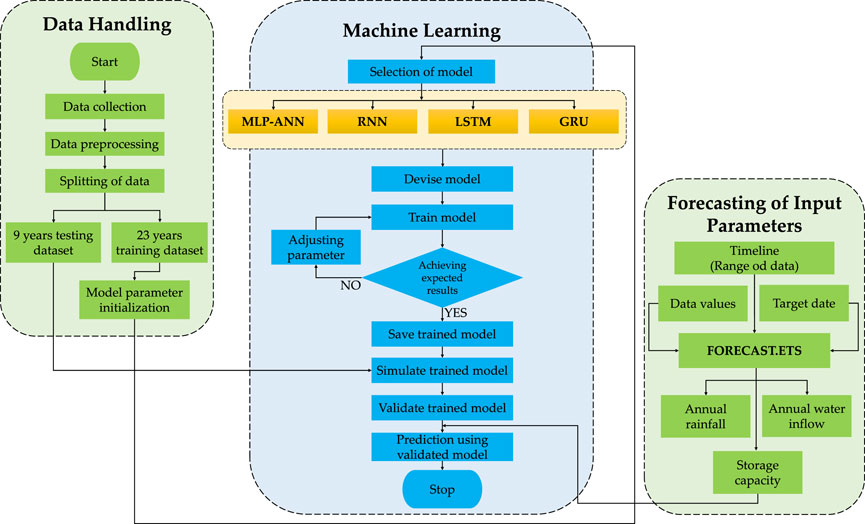
FIGURE 1. Process flow diagram for pre-processing of data and applying machine learning models to validate and forecast sediment deposition inside reservoir based on the forecasted features influencing the sediment volume.

2.1 Study area and data collection

Jothiprakash and Garg (Jothiprakash and Garg, 2009) chosen the Gobindsagar Reservoir at the Bhakra Dam on the Satluj River in the Himachal Pradesh district of Bilaspur, India, to examine sedimentation. One of India’s oldest dams, the Bhakra dam was built in the foothills of the Himalayas, resulting in the construction of the Gobindsagar reservoir. Devastating floods have been contained, and the advantages of irrigation and power have significantly increased wealth in the area. It has a planned 9,867.84×10⁶ m³ of total storage space. At full reservoir level, the reservoir’s huge water spread area measures 168.35 km², and its catchment area is 56,876 km². The river Satluj, which flows over difficult terrain and originates from Mansarover Lake, conveys a significant amount of silt into the reservoir. The area experiences high levels of sediment transport due to the steep terrain, poor structural characteristics of the soils, clay-rich rocks, and widespread occurrence of limestone deposits. This region frequently has slips and landslides, which could be one of the main sources of sediment in the river.

In addition to the yearly basis rainfall, inflow of water, and the storage capacity, the study performed by Jothiprakash and Garg (Jothiprakash and Garg, 2009) used data for the years 1971–2003. Figures 2A–C represents the yearly variation of influencing factors while Figure 2D shows the accumulation of sediments inside the reservoir each year. The time series plot of these data in Figure 3 shows the relationship between the primary y-axis factors, the rainfall (R_a), water inflow (I_w), and the storage capacity (C_r) against the actual volume of sediment (S_v) deposited inside the Gobindsagar reservoir shown in blue on the secondary y-axis. The straight lines show the linear trends along with the equations of lines in their respective legends of all the influencing parameters and the volume of sedimentation to check the relationship between influencing parameters and the actual volume of sedimentation retained inside the Gobindsagar reservoir. With the increase of water inflow, volume of sediments also increases. Consequently, it is possible to assert that there is a correlation between inflow and sediment volume. Even though the yearly basis rainfall and storage capacity data do not strongly correlate with the sediment volume, these factors were still employed in the current investigation because they were regarded as important factors in past sedimentation studies. From Figure 3, it can also be concluded that, due the impact of all the factors on sediment volume, it is hard to get explicit combined relationship of all the factors impacting sediment volume. It is therefore recommended to employ advanced machine learning approaches instead of basic linear or multivariate regression models.

FIGURE 2

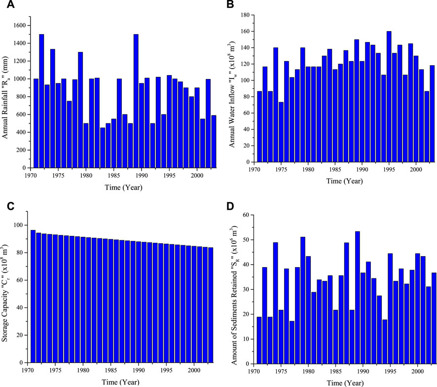
FIGURE 2. Yearly basis data used for the estimation of sediments retained inside the Gobindsagar reservoir from year 1971 to year 2003 using three influencing factors of (A). Rainfall, (B). Water inflow and (C). Storage capacity of the reservoir, (D). Actual amount of yearly sediments accumulated inside the Gobindsagar reservoir.

FIGURE 3

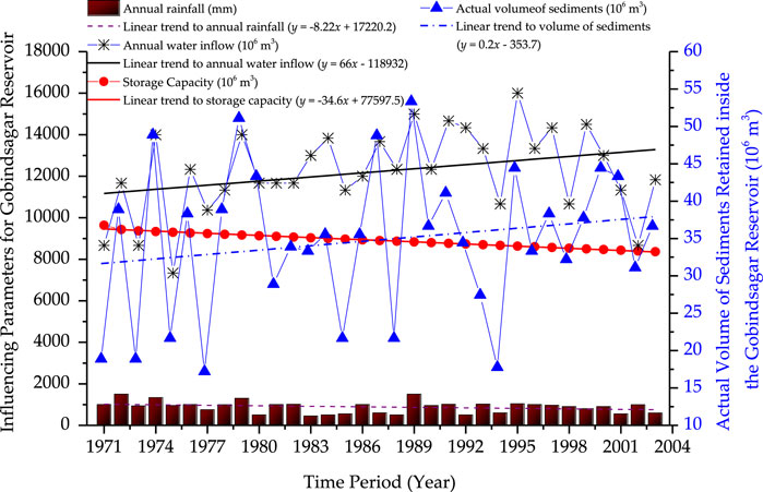
FIGURE 3. Time series plot of influencing parameters including yearly basis rainfall, water inflow, and the storage capacity used for the estimation of sediments retained inside the Gobindsagar reservoir from the year 1971 to the year 2003.

2.2 Development of machine learning models

2.2.1 Multi-layered perceptron artificial neural network (MLP-ANN)

An ANN consists of small computational elements known as artificial neurons. These neurons when arranged in a layered structure form are known as multilayered perceptron artificial neural networks. The outer layers in MLP-ANN are referred to as the input and output layers, respectively, based on where we supply our input variables and where we obtain our output variables. The number of neurons in these layers is fixed and dependent on the number of input features and the number of output parameters. The layers between both the input layer and the output layer are known as hidden layers, and the artificial neurons that lie within it are known as hidden neurons. The number of hidden layers and neurons in each hidden layer can be changed, and the computational cost of a neural network model is affected by these numbers. Neural networks are named according to the number of hidden layers and neurons in each hidden layer. The typical N3-45-45-1 neural network structure, for example, indicates that the network has four layers: one input layer, one output layer, and two hidden layers. It also represents that there are input layers consisting of 4 neurons, both the first and second hidden layers consist of 45 neurons and the output layer contains only 1 neuron. Artificial neural network modelling in MATLAB was done through trial and error. The number of neurons in each hidden layer as well as the total number of hidden layers were changed, and the best suitable structure that predicted the outcomes with the least amount of error was selected. Figure 4 depicts the typical architecture of the N3-45-45-1 network proposed to predict the sediment volume inside the reservoir.

FIGURE 4

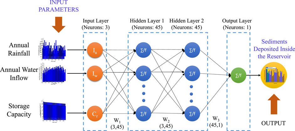
FIGURE 4. Typical neural network architecture (N4-45-45-1) describes four layers: one input layer consisting of 3 neurons, one output layer with 1 neuron, and two hidden layers with 45 neurons each.

2.2.2 Recurrent neural network

The recurrent neural network is a type of artificially intelligent neural network designed to analyze sequential input (RNN). The RNN builds connections between time steps and circulates weights among them in various time steps. When users want to execute prediction operations on sequential or time-series based data, they use recurrent neural networks, a type of ANN. Ordinal or temporal issues are frequently addressed by these deep learning layers. RNNs are built with memory so they can use any data from previous inputs to affect the input and output at the moment. The same training techniques are used for this network. RNN generates the output depending on past input and its context, unlike classic neural networks, which believe that input and output are independent of one another. RNN shares parameters with each layer of the network, which is another distinct feature. Recurrent neural networks share a single weight parameter throughout all network layers, unlike feedforward networks, which provide separate weights to each node.

Figure 5 displays the RNN structure with one hidden layer. In contrast to multilayer perceptrons, the RNN hidden layer is connected with both the hidden layer nodes and the output layer. This causes RNN to create a non-linear relationship between the sequential data collected at various periods in addition to reducing the number of parameters. RNN is hence uniquely advantageous in solving non-linear and time series problems. The present RNN uses 7 neurons in the hidden layer and 1 neuron in the output layer, both of which use the Rectified Linear Unit (ReLU) as an activation function for hidden layer and the sigmoid activation function for output layer. Recurrent neural network model in MATLAB was applied using a trial and error strategy. The number of neurons in each hidden layer as well as the total number of hidden layers were changed, and the best structure that predicted the outcomes with the least amount of error was selected. A typical RNN architecture (R3-7-1) is shown in the figure below.

FIGURE 5

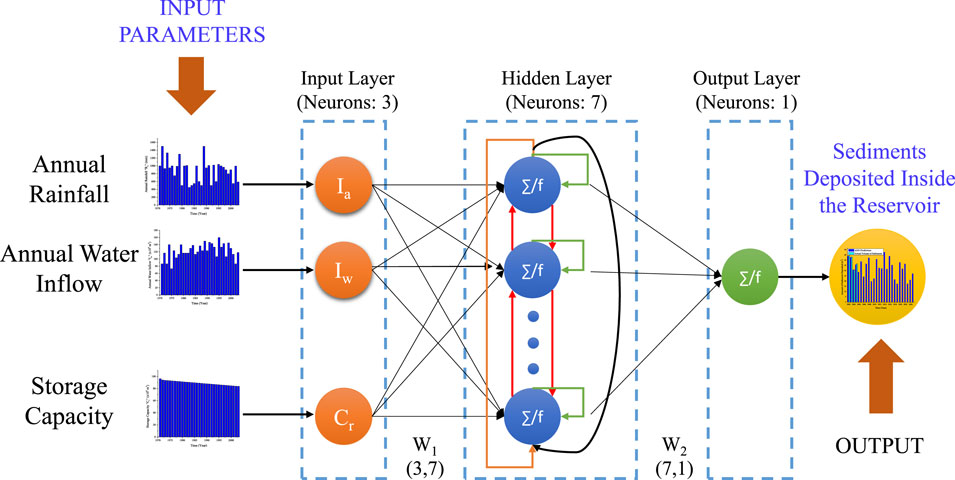
FIGURE 5. RNN structure (R3-7-1) diagram with one hidden layer containing 7 neurons.

2.2.3 Long-short term memory neural network

A conventional RNN network tends to lose information when exposed to extended sequences or phrases because it cannot store the long sequences and because the algorithm only considers the most recent information that is available at the node. Vanishing gradients is the term used to describe this issue. When using RNN to train networks, we backpropagate through time while calculating the gradient at each time step or loop operation and updating the network weights as a result. Now the relative gradient is calculated to be modest if the layer is not significantly affected by the prior sequence. When dealing with longer sequences, we see that if the gradient of the previous layer is smaller, the weights that must be applied to the context are also reduced. As a result, the network does not learn the impact of earlier inputs, leading to the short-term memory issue. Specialized RNN versions like LSTM and GRU are developed to address this issue.

The long-short term memory (LSTM) neural network a significant advancement over the recurrent neural network. It can successfully address the issues of RNN gradient explosion and disappearance and improve the network’s memory capacity. Additionally, the LSTM network, which has both an internal “LSTM cell” circulation and an exterior RNN cycle structure, can retain longer historical data information. As a result, the affine translation of input and loop units is not simply imposed by LSTM as an element by element non-linearity (Liu et al., 2021). In the present LSTM model, 2 hidden LSTM layers with 4 LSTM neurons in each hidden layer are used. The LSTM model was applied in MATLAB through a trial-and-error process. The number of hidden layers and the number of neurons within each hidden layer were changed, and the best structure that predicted the outcomes with the least amount of error was selected. The typical architecture of LSTM (L3-4-4-1) is shown in Figure 6A. Figure 6B depicts the LSTM hidden layer’s structural layout. The hidden layer node of the current sequence has $x_t$ as its input, $C_t$ as its hidden layer node state, $h_t$ as its hidden layer node’s output, $\sigma$ as its non-linear activation function of sigmoid, and $\tan h$ as its hyperbolic tangent function. $x_t$ is the input, and C_t-1 and h_t-1 are the node states of the previous hidden layer sequence. While LSTM networks have more complex structures, more parameters, and slower convergence speeds than RNNs, they are superior at learning the long-term relationship between sequential data.

FIGURE 6

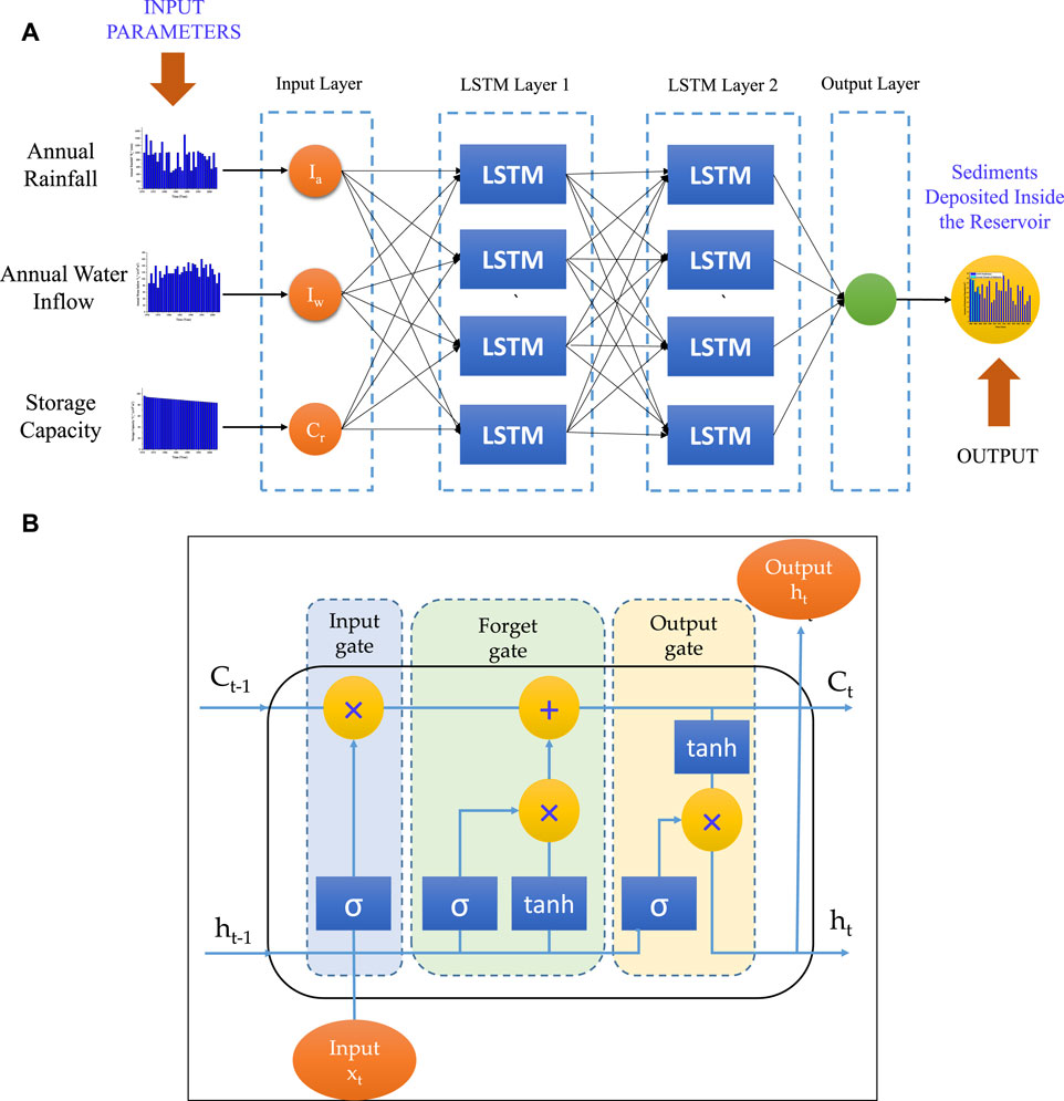
FIGURE 6. (A). The proposed LSTM network with two LSTM layers and four hidden layer LSTM neurons, (B). Hidden layer structure of LSTM with input gate using sigmoid activation function, forget gate and output gate using activation functions: sigmoid and $\mathit{tanh}$

2.2.4 Gated recurrent unit neural network

The gated recurrent unit (GRU) neural network is an improvement and up-gradation of the long-short term memory (LSTM) network. It carries over the LSTM network’s capacity to handle time series and non-linear issues. Additionally, it keeps the LSTM network’s memory unit function while simultaneously streamlining the structure and lowering the number of parameters, which significantly accelerates training. In the present GRU model, 2 hidden GRU layers with 3 GRU neurons in each hidden layer are used along with the sigmoid activation function in the output layer. Trial and error was used to apply the GRU model in MATLAB. The optimal structure that predicted the results with the least amount of error was chosen after varying the number of hidden layers and the number of neurons within each hidden layer. Figure 7A depicts the typical GRU (G3-3-3-1) architecture. The structure of the GRU neural network is shown in Figure 7B, where $u_t$ denotes the update gate state, $r_t$ the reset gate state, and $h_t$ the neuron’s awaiting output. The GRU neural network builds on the LSTM network by improving the “gate” design and optimizing it to a cell structure with two “Gates” rather of the original cell structure’s three “Gates”. The reset gate and the update gate are the basic components of the gating cycle unit. The $r_t$ and $u_t$, respectively, are defined as the reset gate and up-date gate states at time $t$ (Goh, 1995; Liu et al., 2022).

$r_t=\left(\sigma W_r{x}_t+Z_r{h}_{t-1}\right)(1)$

$u_t=\left(\sigma W_u{x}_t+Z_u{h}_{t-1}\right)(2)$

where $x_t$ is the input data and $W$ and $Z$ are weight matrices. The following formulations are used to compute the candidate hidden state $h_t$ and the hidden state $\stackrel{\sim }{h_t}$:

$h_t=\left(1-u_t\right)h_{t-1}+u_t\stackrel{\sim }{h_t}(3)$

$\stackrel{\sim }{h_t}=\tan h\left[W_h{x}_t+\left(r_t{*h}_{t-1}\right)\right](4)$

FIGURE 7

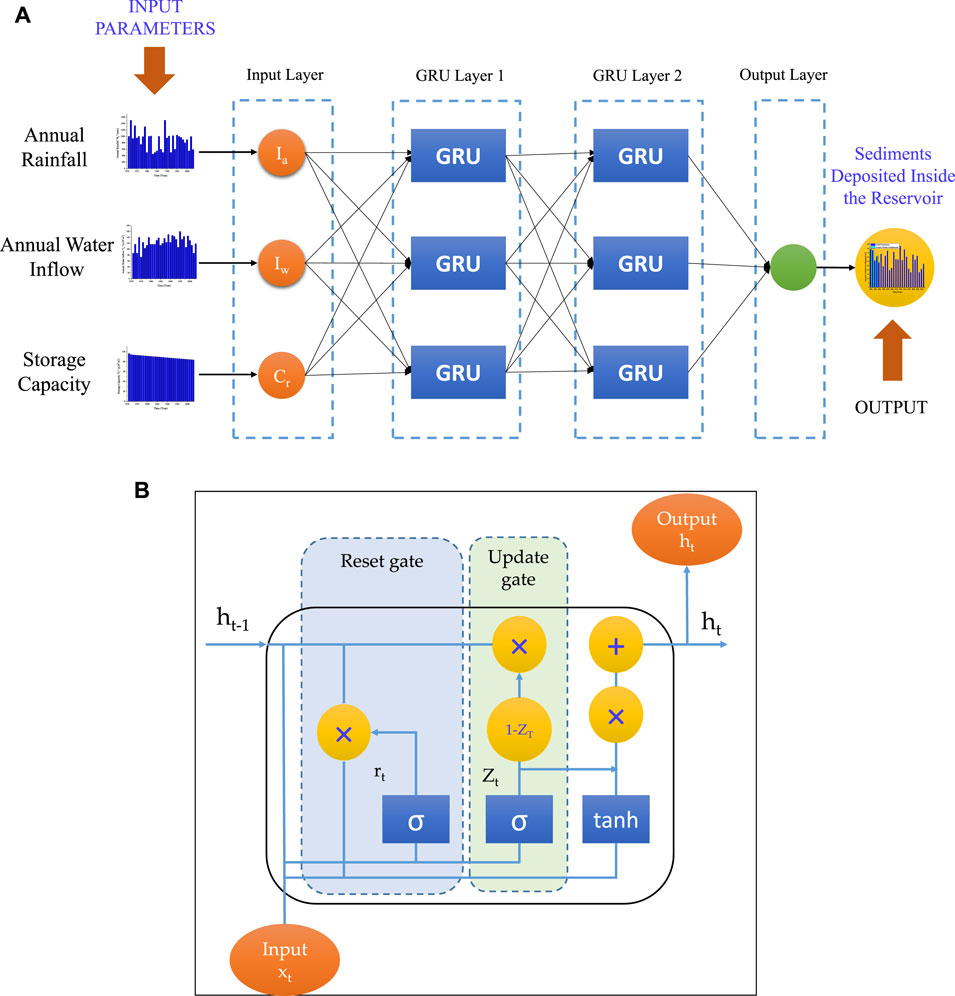
FIGURE 7. (A). The proposed GRU network with two GRU layers and three hidden layer GRU neurons, (B). Schematic diagram of GRU network’s hidden layer where sigmoid activation function is used in the reset gate and update while $\mathbf{tan}\mathit{h}$ is used for the output.

Equations 5, 6 contain two distinct activation functions that can be described as follows:

$\sigma \left(x\right)=\frac{1}{1+\mathit{exp}\left(x\right)}(5)$

$\tan h\left(x\right)=\frac{1-\mathit{exp}\left(2x\right)}{1+\mathit{exp}\left(x2\right)}(6)$

Utilizing a getting mechanism to learn long-term dependencies is fundamentally similar to using LSTM. The GRU has two gates, while the LSTM has three, which is one of the few points of difference. There is no internal memory in the GRU, and there is no output gate like there is in the LSTM. While in GRU the prior hidden state is directly affected by the reset gate, in LSTM the input gate and target gate are coupled by an update gate. The input and target gates in an LSTM take on the role of the reset gate. According to how both layers, LSTM and GRU, operate, LSTM is more accurate on a larger dataset whereas GRU utilises fewer training parameters, uses less memory, and executes more quickly. When dealing with lengthy sequences and accuracy is a requirement, LSTM is an option; GRU is employed when less memory use and quicker results are desired.

2.2.5 ETS forecasting model

A technique for time series univariate forecasting is the ETS (Error, Trend, and Seasonal) method. The flexibility of the model to trend and take into account seasonal components of numerous parameters is what makes it flexible. With the exception of the annual water inflow, there is no general trend for the input values, hence the approach is utilized. The ETS model is best suited for data without a clear trend. The exponential smoothing process is used by the ETS function to forecast future values. Excel’s FORECAST tool uses linear regression to forecast a future value. In other words, FORECAST extrapolates a value from the past along a line of best fit. The FORECAST function has the following syntax:

$FORECAST\left(X_{required},y_{actual},x_{actual}\right)(7)$

Where, $X_{required}$ is a numerical $x$-value for which one can forecast a new $y$-value. The actual $y$'s and actual $x$'s arrays of known dependent and independent $y$-values and $x$-values, respectively, are both necessary. In the present study, the actual $x$'s are the yearly basis input features of rainfall (R_a), inflow of water (I_w) and the storage capacity (C_r) of the Gobindsagar reservoir and the actual $y$'s are output values of yearly basis sediment volume (S_v) inside the Gobindsagar reservoir.

2.2.6 Models training

For the validation of proposed machine learning models for Gobindsagar reservoir, randomly chosen 23 years of data was used for training and randomly chosen 9 years of data was used for validation purposes.

The neural network model’s major parameters, such as the number neurons in the hidden layer and the number of hidden layers, must be optimized and adjusted during the training process of each proposed neural net model of this study. Theoretically, the model performs better and makes more accurate predictions the deeper and more complicated the network is. This is because there are more hidden layers and neurons. However, certain research has demonstrated that having too many hidden layers and neurons would cause training issues and over fitting, which will lower the model’s predictive accuracy. If the network is too shallow and straightforward, it will likely result in inadequate fitting and fall short of the required standards. As a result, the network’s ability to predict the future depends greatly on the chosen number of hidden layers and number of neurons. We must find a balance between the network’s capacity for learning and the complexity of the training process as well as the demands of prediction accuracy. Based on our experience and numerous experimental findings, we must choose the right number of nodes and hidden layers (Jothiprakash and Garg, 2009; Mohammadi et al., 2021b). Additionally, the model’s complexity can be somewhat reduced as well as its convergence speed and prediction accuracy by optimizing training parameters consisting of the learning rate, batch size, and a maximum number of iterations. In the present study, a typical optimized neural network architecture N3-45-45-1 with resilient propagation as a training function was used to train the MLP-ANN. For basic RNN architecture (R3-7-1), rectified linear unit as an activation function and 1 neuron in the output layer were used for training purposes. The two-layer LSTM neural network model’s topology (L3-4-4-1) is used in the present study. Input, hidden, and output layers are all included in neural network models, with the hidden layer serving as the network’s structural backbone. Long-term memory is a capability of GRU neural network. The GRU network model can successfully limit the impact of these interactions by addressing the long-term reliance on series data, and its inbuilt control mechanism can automatically learn time-series characteristics. The two-layer GRU neural network model’s topology (G3-3-3-1) is used in the present study.

2.3 Performance evaluation of proposed models

To test and train data sets for the MLP-ANN, RNN, LSTM, and the GRU network models, all data are initially standardized to range from 0 to 1 using Equation 8. Additionally, the preprocessing that increased the calculation speed of network approaches may ensure the convergence of neural nets.

$x_{normalized}=\frac{x-x_{\mathit{min}}}{x_{\mathit{max}}-x_{\mathit{min}}};x=R_a,I_w,C_r,S_v(8)$

where, $x$ is the original data for the annual rainfall ($R_a$), annual water inflow ($I_w$), storage capacity ($C_r$) and sediment volume ($S_v$) and; $x_{normalized}$ is the normalized data for the above mentioned three input parameters and the sediment volume; and ${\mathrm{x}}_{\max }$ and ${\mathrm{x}}_{\min }$ respectively, represent the maximum and minimum of the original dataset of $R_a,I_w,C_r,$ and $S_v$.

The performance of machine learning models were compared using various statistical indicators such as correlation coefficient (R), mean absolute error (MAE), variance accounted for (VAF), mean squared error (MSE), and root mean square error (RMSE). Furthermore, these performance metrics may provide insight into how well the forecasting model performed in terms of reference value. The following equations provide the mathematical expressions of previously mentioned common statistical indicators:

The following is a description of R criteria:

$R=\sqrt{1-\frac{{{\displaystyle \sum }_{i=1}^n\left[{\left(\widehat{S_v}-S_v\right)}_i\right]}^2}{{\displaystyle \sum }_{i=1}^n{\left(\widehat{S_v}\right)}_i^2-\left(\frac{1}{n}\right){\displaystyle \sum }_{i=1}^n{\left(\widehat{S_v}\right)}_i^2}}(9)$

The following is an illustration of MAE criteria:

$MAE=\left(\frac{1}{n}\right){\displaystyle \sum }_{i=1}^n{\left(\widehat{S_v}-S_v\right)}_i(10)$

When the mean squared error reached the stopping criteria, i.e. $1\times {10}^{-6}$ with respect to weights and biases, the training process was terminated. The mean squared error was estimated using Equation 11 depending on the network prediction ($\widehat{S_v}$) and the target value ($S_v$). For future simulations, the optimized weights and biases were saved.

$\mathrm{M}\mathrm{S}\mathrm{E}=\left(\frac{1}{n}\right){\displaystyle \sum }_{i=1}^n{\left[{\left(\widehat{S_v}\right)}_i-{\left(S_v\right)}_i\right]}^2(11)$

By comparing the assessed values and the model’s evaluated output, VAF is typically used to gauge a model’s correctness. The following Equation 12 can be used to calculate the VAF criteria:

$VAF=\left(1-\frac{var\left[{\left(\widehat{S_v}\right)}_i{-\left(S_v\right)}_i\right]}{var\left[{\left(\widehat{S_v}\right)}_i\right]}\right)\times 100\%(12)$

The RMSE is typically used to track the accuracy of the model’s error function. As RMSE decreases, the model’s performance improves. Equation 13 can be used to calculate the RMSE criteria as follows:

$RMSE=\sqrt{\left(\frac{1}{n}\right){\displaystyle \sum }_{i=1}^n{\left[{\left(\widehat{S_v}\right)}_i-{\left(S_v\right)}_i\right]}^2}(13)$

In machine learning, the accuracy of a model can also be evaluated using the Mean Absolute Percentage Error (MAPE). The MAPE is a loss function that specifically identifies the error of a certain model. Finding the absolute difference between the actual and predicted values, then dividing by the actual value, yields the MAPE. The mean is calculated by adding these ratios for all values. Equation 14 can be used to calculate the MAPE criteria as follows:

$MAPE=\sqrt{\left(\frac{1}{n}\right){\displaystyle \sum }_{t=1}^n\left|\frac{{\left(S_v\right)}_t-{\left(\widehat{S_v}\right)}_t}{{\left(S_v\right)}_t}\right|}(14)$

where $S_v$ is the actual sediment load deposited inside the reservoir, $\widehat{S_v}$ stands for the predicted sediment load deposited inside the reservoir, and $n$ is the number of testing data points for equations (9) through (14).

2.4 Sensitivity analysis of influencing factors

Firstly, the sensitivity of each influencing factor in predicting the sediment volume was measured using an evaluation approach based on the weight matrix of the suggested optimized network and Garson’s modified equation (64). The computational formula is given in the equation below:

$S_j=\frac{{\displaystyle \sum }_{m=1}^{N_h}\left[\left(\frac{\left|w_{jm}^{ih}\right|}{{\displaystyle \sum }_{k=1}^{N_i}\left|w_{km}^{ih}\right|}\right)\times w_{mn}^{ho}\right]}{{\displaystyle \sum }_{k=1}^{N_i}\left[{\displaystyle \sum }_{m=1}^{N_h}\left(\frac{\left|w_{km}^{ih}\right|}{{\displaystyle \sum }_{k=1}^{N_i}\left|w_{km}^{ih}\right|}\right)\times w_{mn}^{ho}\right]}(15)$

Where, the indices $i$, $h$, and $o$ represents the input, hidden and the output layers respectively, and the indices k, m, and n represents the input, hidden and the output layer’s neurons, respectively, $S_j$ denotes the relative significance of the jth influencing factor on the output variable, $N_i$ and $N_h$ denote the number of neurons in the input and output layers, respectively, and $W$ denotes connected weights. All connection weights were given their absolute values in the modified Garson approach to avoid the opposing effects of positive and negative values (Taylor, 2001).

Secondly, the sensitivity of each influencing factor was evaluated using Olden’s algorithm, which suggested that the connection weight approach consistently identified the correctly ranked significance of all predictor variables. The weights are provided by the MLP-ANN model (N3-45-45-1) utilized in this investigation between artificial neurons.

Thirdly, a perturbation method is implemented for RNN-based models including simple RNN model (R3-3-7-1), LSTM model (L3-4-4-1), and GRU model (G3-3-3-1), the importance of each influencing factor is measured. A time series with the three features R_a, I_w, and C_r serves as the input data for the current RNN, LSTM and GRU models. A time series is the S_v target variable for all the three models. The output is dependent on all three features, as is obvious. The outcomes of different methodologies used to determine the variable importance should be logically validated by a good variable importance measure, which should display an appropriate ranking. A sample size of 23 years of data is used to calculate the model’s predictions, or S_v, in order to determine the variable’s significance. Then, for each input variable, perturbation is performed using a random normal distribution centered at 0 with scale 0.5 and computes a prediction S_v. By calculating the difference in Root Mean Square between the original value of $S_v$ and the perturbed value of $\widehat{S_v}$, the impact of this perturbation can be improved. That variable is “more important” if there is a bigger difference in the Root Mean Square. Of course, your specific dataset will have a significant impact on the exact method you use to perturb your data and how you determine the difference between perturbed and unperturbed results.

3 Numerical results

Jothiprakash and Garg used 33 years of data i.e. 1971 to 2003 and the basic neural network model to estimate the sediment volume deposited inside the Gobindsagar reservoir in India using three yearly basis influencing factors i.e. rainfall, and inflow of water and storage capacity. The reference paper used randomly selected data for 23 years for training and 9 years for validation of the ANN model. For the data provided in the paper, the machine learning models described above were used to develop the typical network structures of MLP-ANN, RNN, LSTM, and GRU. It was found that the N3-45-45-1, R3-7-1, L3-4-4-1, and G3-3-3-1 produced superior outcomes as compared to the model used in the reference paper (Jothiprakash and Garg, 2009). In Table 1, the outputs of each model are compared with the actual sediment volume within the Gobindsagar reservoir. The results demonstrate that the proposed MLP-ANN, RNN, LSTM, and GRU models, respectively, may produce better results with maximum errors reduced from 24.6% to 8.05%, 7.52, 1.77, and 0.05. Additionally, it was noted that each prediction’s error was lower than that of the reference model. For the error analysis, it can also be seen that the GRU model predicts better results as compared to the reference model, and all the other models presented in this study. Figure 8A depicts the comparison of actual volume of sediments deposited inside the Gobindsagar reservoir with reference neural network model and proposed machine learning models using tested data from year 1971 to year 1999 while in Figure 8B it can be seen that the relative errors estimated using GRU model are lying between -0.5% and 0.5% inside the grey rectangle and showing the better results as compared to the other models.

TABLE 1

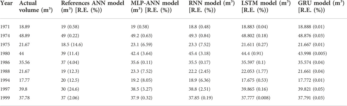
TABLE 1. Validation of the proposed ANN model against the reference ANN model and the actual sediment volume inside the Gobindsagar reservoir.

FIGURE 8

FIGURE 8. (A). Comparison of actual volume of sediments retained inside the Gobindsagar reservoir with reference ANN model and proposed machine learning models using tested data from year 1971 to year 1999, (B). Reduction in relative error of proposed machine learning models in comparison with the reference model.

In the validation, the proposed machine learning neural network models were concluded better than the reference ANN model (Jothiprakash and Garg, 2009) and further it was found that the GRU performs best as compared to others. Therefore, the proposed models were used to forecast the sediment volume inside the Gobindsagar reservoir in the next 22 years i.e. 2003 to 2025. The actual $y$’s and actual $x$’s arrays of known dependent and independent $y$-values and $x$ values, respectively, are included in the already known data and are both required for the input of the function specified in Equation 7. In the current study, the actual‘s are the annual input features of rainfall ($R_a$), water inflow ($I_w$), and storage capacity ($C_r$) of the Gobindsagar reservoir, and the actual $y^{\prime }$ s are output values of annual basis sediment volume ($S_v$) within the Gobindsagar reservoir. Using the actual $x$’s and actual $y$’s for the previous 33 years, the ETS forecasting model predicted the input parameters for the following 22 years from year 2003 to year 2025. Figure 9A,C depict the three yearly forecasted influencing factors for the Gobindsagar reservoir: rainfall, inflow of water, and storage capacity. Figure 10A through Figure 10D show the results of forecasts for the sediment volume that will be deposited inside the reservoir over the course of the next 22 years using the proposed machine learning models MLP-ANN, RNN, LSTM, and GRU respectively. In Figure 10A–D, the forecasts are also compared with data on the actual sediment load deposited that were taken from references for the years 2000–2003. The figure makes it evident that forecasts for this years’ sediment deposition are rather close to being accurate.

FIGURE 9

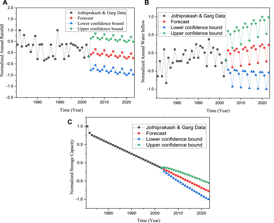
FIGURE 9. Forecasted input parameters for the Gobindsagar reservoir including (A) normalized rainfall; (B) normalized inflow of water and (C) normalized storage capacity.

FIGURE 10

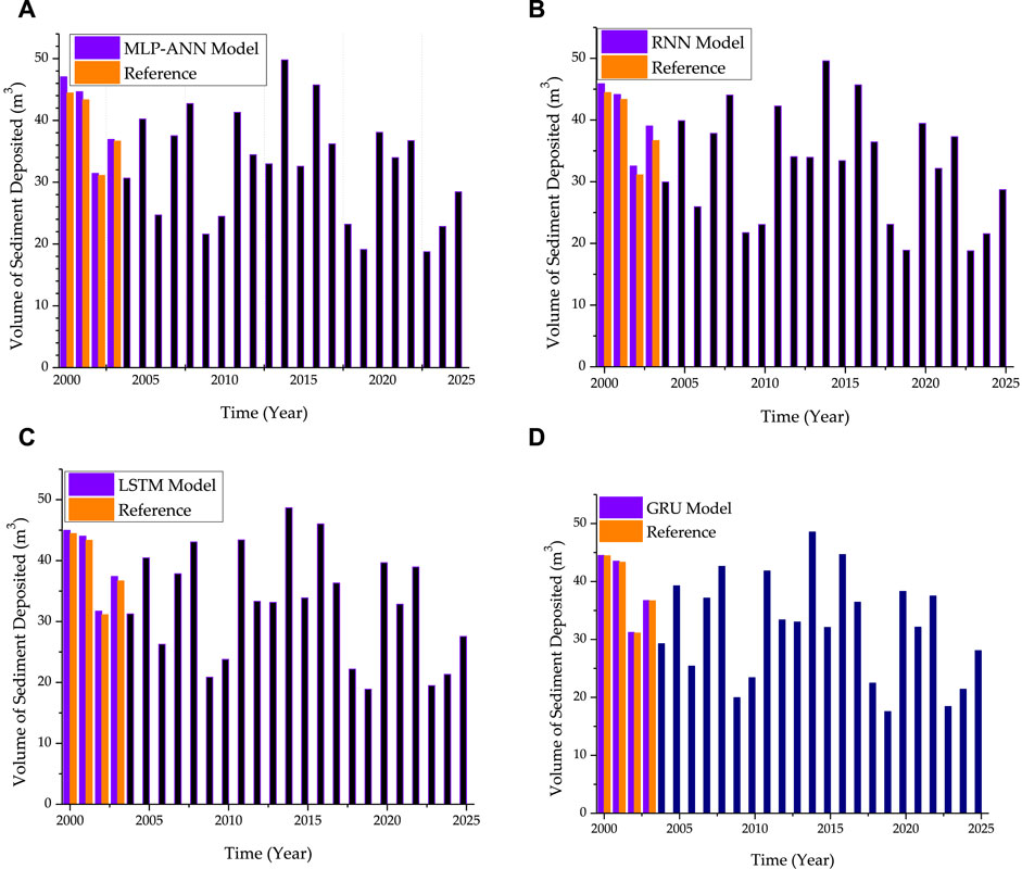
FIGURE 10. Sedimentation prediction for next 22 years using proposed machine learning models (A) MLP-ANN, (B) RNN, (C) LSTM, and (D) GRU, based on the three forecasted input parameters.

Eventually, the statistical indicators mentioned previously were also employed to carry out this comparison and outcomes of this comparison were presented in Table 2. What can be shown in Table 2 was that the four kinds of sediment prediction models based on machine learning method were far superior to that established in the reference model in their prediction accuracy. It can be clearly seen that the LSTM and GRU models were superior to the MLP-ANN and RNN model in prediction precision by comparing the prediction precision of the four types of machine learning models (MLP-ANN, RNN, LSTM, and GRU) established in this study, among which GRU took the best precision due to the highest R of 0.9654 and VAF of 91.7689, the lowest MAE of 0.7777, the lowest RMSE of 1.1522 and the lowest MAPE of 0.3786%. Through the comparison between the prediction precision of LSTM and GRU, there was just slight discrepancy between their precision.

TABLE 2

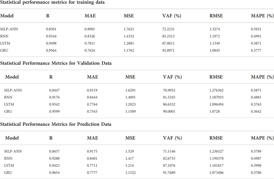
TABLE 2. Comparing the performance of the MLP-ANN, RNN, LSTM, and GRU models using five performance metrics-correlation coefficient (R), mean absolute error (MAE), mean squared error (MSE), variance accounted for (VAF), root mean square error (RMSE) and mean absolute percentage error (MAPE) for training data, validate data and prediction data.

To conclude, both LSTM and GRU models could provide a successful sediment volume prediction performance. The GRU model showed a higher precision in predicting sediment volume and from Table 2 which we can conclude that GRU modeled in this study took a higher efficiency in predicting the sediment volume with its high precision. Figures 11A–C show the graphical depiction of the performance indicators for all the machine learning models for training data, validation data and the prediction/test data respectively implemented in this study, where the primary y-axis tells the variation of R, MAE, MSE, RMSE, MAPE and the secondary y-axis in purple color represents the variation in VAF with purple error bars along with the labeled values of VAF in black. From figure, it can also be seen that LSTM and GRU perform better.

FIGURE 11

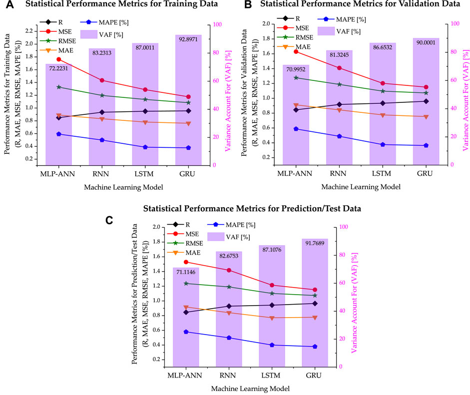
FIGURE 11. Performance indicators for all the machine learning models for (A). Training data, (B). Validation data, (C). Prediction/test data: where the primary y-axis tells the variation of R, MAE, MSE, RMSE, MAPE for each model and the secondary y-axis in purple represents the variation in VAF with purple error bars for each model along with the labeled VAF.

Table 3 represents the hyperparameters settings for the optimized applied machine learning models.

TABLE 3

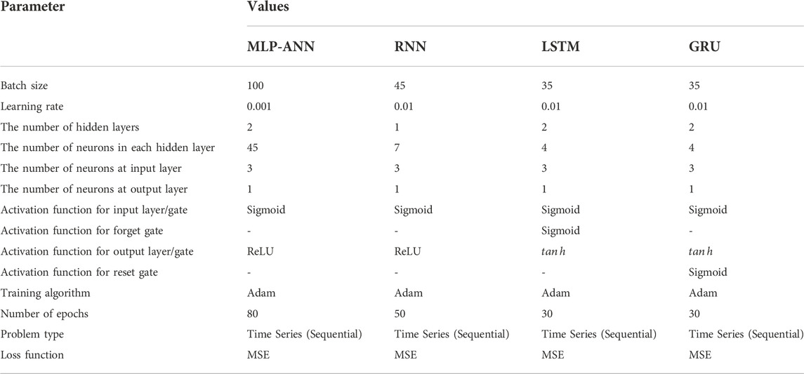
TABLE 3. Hyperparameters tuning for applied machine learning models.

Taylor diagrams can be used as a graphical representation of how well a model (or group of patterns) matches the data. To assess how similar two or more patterns are, the correlation, the centered root-mean-square difference, and the standard deviations are employed. When comparing the relative capabilities of several models or analyzing various aspects of complicated models, these diagrams are especially useful. The correlation coefficient, root mean square difference (RMSD), and standard deviation are all represented by a Taylor diagram in Figure 12. The cosine rule between the three-centered data was used to construct this picture, which shows how closely trends resemble one another (Liu et al., 2022). A blue circle on the bottom line, which acts as the reference, designates the position of the observation. Since the correlation is visible on the azimuthal axis, values that are closer to 1 are preferable. The radial distance from the origin is shown by black dashed lines with the standard deviation; again, the closer to 1 the better. Since the root mean square errors are displayed as the radial distance from the origin by green dashed lines, the lowest distance to the observed position is regarded as the best. The accompanying Taylor diagram demonstrates that the proposed GRU model (shown with a green circle) has one of the lowest RMSD values and the highest correlation values. Additionally, in relation to the reference point, its standard deviation is one of the lowest. Then, the proposed LSTM model (shown with a purple circle) has one of the second lowest RMSD values and the second highest correlation values. Additionally, in relation to the reference point, its standard deviation is one of the second lowest. On the basis of RMSD’s, correlation coefficients and the standard deviations, it can be concluded that the proposed GRU model is the best model, then LSTM performs better, RNN performs good and the MLP-ANN model performs reasonably good.

FIGURE 12

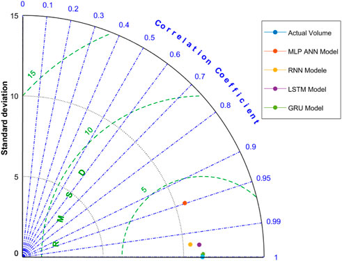
FIGURE 12. Taylor Diagram for the evaluation of model performance, where black dotted arcs represent the standard deviation, green dashed arcs represent the root mean squared difference, and blue dotted lines represent the Pearson’s correlation coefficient (R), and the different colored dots represents the model performances.

The sensitivity analysis of each influencing factor in predicting the sediment volume deposited for the Gobindsagar reservoir was measured using an evaluation approach based on the weight matrix of the suggested optimized network and Garson’s modified equation, Olden’s algorithm, and perturbation method discussed above in Section 2.1.7. Figure 13A represents the results obtained by Garson’s modified equation and the Olden et al. approach for MLP-ANN model used in this study. It can be seen that most critical parameter in predicting the annual sediment volume was the annual rainfall whereas the least critical was annual inflow of water. Figure 13B represents the outcomes obtained from perturbation method used for all the RNN based neural network architectures implemented in this study. It is obvious from the figure that using perturbation method for the basic RNN (R3-7-1), LSTM (L3-4-4-1), and GRU (G3-3-3-1) structures, the sediment volume is most sensitive to the annual rainfall based on the highest perturbation effect whereas it is least sensitive to the annual inflow of water. The ranking of the influencing factors is given below;

$\mathrm{A}\mathrm{n}\mathrm{n}\mathrm{u}\mathrm{a}\mathrm{l}\mathrm{R}\mathrm{a}\mathrm{i}\mathrm{n}\mathrm{f}\mathrm{a}\mathrm{l}\mathrm{l}\left({\mathrm{R}}_{\mathrm{a}}\right)>\mathrm{A}\mathrm{n}\mathrm{n}\mathrm{u}\mathrm{a}\mathrm{l}\mathrm{W}\mathrm{a}\mathrm{t}\mathrm{e}\mathrm{r}\mathrm{I}\mathrm{n}\mathrm{f}\mathrm{l}\mathrm{o}\mathrm{w}\left({\mathrm{I}}_{\mathrm{w}}\right)>\mathrm{S}\mathrm{t}\mathrm{o}\mathrm{r}\mathrm{a}\mathrm{g}\mathrm{e}\mathrm{C}\mathrm{a}\mathrm{p}\mathrm{a}\mathrm{c}\mathrm{i}\mathrm{t}\mathrm{y}\left({\mathrm{C}}_{\mathrm{r}}\right)$

FIGURE 13

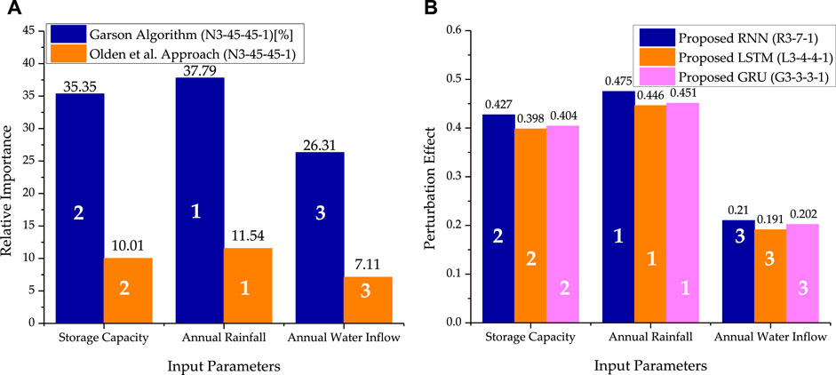
FIGURE 13. The relative importance of each influencing factor in predicting the sediment volume deposited inside the reservoir which is assessed for MLP-ANN using (A) Garson’s Algorithm and Olden’s algorithm of connection weights (B) perturbation method for RNN, LSTM and GRU.

4 Discussion

The main objectives of this study were to validate the proposed machine learning models including MLP-ANN, RNN, LSTM and GRU for the Gobindsagar reservoir in India based on the three input features i.e., annual rainfall (R_a), annual inflow of water (I_w) and the annual storage capacity (C_r) of the Gobindsagar reservoir and one output of sediment volume (S_v). The accurate future prediction of the sediment volume and the sensitivity analysis of each influencing factor was performed using above mentioned machine learning approaches. On the basis of the numerical comparison of results with the actual sediment volume presented in Table 1, it was found that the proposed models perform better as compared to the reference model. The prediction’s error were observed to be lower than that of the reference model. The sediment volume was predicted more precisely on the basis of the good performance of GRU model as compared to other implemented models. The performance of the GRU model can also be ensured from the Taylor’s diagram as shown in Figure 12. Using perturbation method, the sediment volume was found to be the most sensitive to the annual rainfall based on the highest perturbation effect whereas it is least sensitive to the annual inflow of water.

Apart from the typical objectives of the present study, it can be further assessed that under specific circumstances, accumulated sediments can have an impact on a river’s usual hydrological system. The sediments may begin to accumulate at the river channel’s bottom and in result, the river channel’s bottom becomes elevated, reducing its cross-sectional area and choking the river’s hydrological system. In case of Gobindsagar reservoir which has a capacity to store water up to 9.34 billion cubic meters, the available data sources tell that the amount of sediment has been accumulated up to 1.4587 billion cubic meters until year 2003. This accumulation can be calculated from Figure 2D. Every year, further sediment accumulation may have an impact on hydropower output due to reduced reservoir storage and/or mechanical component failure. If sediments are not properly managed, they can have a harmful effect on the ecosystem and the safety of the reservoir. It is therefore important to accurately predict the amount of sediments inside the Gobindsagar reservoir in the coming years. Based on the available data for the years 1971 to year 2003, the machine learning approaches used in the present study could be able to predict the amount of sediments accumulated every year. Figure 10 shows the sediment volume prediction for next 22 years using proposed machine learning models including MLP-ANN, RNN, LSTM, and GRU, based on the three forecasted input parameters. This could help to check the performance of the best prediction model i.e.; GRU model which calculates the amount of sediments accumulated in the next 22 years i.e.; 0.7028 billion cubic meters. The Gobindsagar reservoir’s yearly sediment deposit frequently disrupts low-level exits, which results in clogging of spillway tunnels or other conduits those may happen as sedimentation progresses. As sediments continue to accumulate, the oxide coating on the blades begins to erode, causing surface irregularities and increasingly severe material degradation that can harm turbines and other mechanical equipment. Extended shutdown times for maintenance or replacement may result from continuous erosion. Last but not least, sediment is a major transporter of suspended contaminants like nitrogen, phosphorus, and heavy metals. The release of sediments as a result of sediment management could have long-lasting repercussions on the environment. The sediment management techniques for reservoir may require to remove already deposited material, reroute some sediment through or around the reservoir, and reduce the quantity of sediment entering the reservoir from upstream. To accomplish these objectives, several reservoir operators have employed sediment management strategies such as bypassing, drawdown routing, dredging, flushing, and erosion control. Because land users might not directly benefit from controlling sediment yield, erosion management is likely the most extensively recommended but least used sediment management strategy. Regarding the hydrological/sediment management significance of this work for stakeholders and local government, further detailed studies and analysis is required and it is also needed to incorporate more hydro-meteorological and catchment details to predict the volume of sediments. These will be studied in the future research and will be highlighted in detail to discuss the significance.

5 Conclusion

The sediment volume inside the Gobindsagar reservoir in India was validated and predicted using multi-layered perceptron artificial neural networks (MLP-ANN), basis recurrent neural networks (RNN), and other types of RNN models, such as long-short term memory (LSTM), and gated recurrent unit (GRU). Firstly, the proposed machine learning models were trained for the data of 23 years and then validated for the tested data of 9 years. It was observed that the proposed models are better in performance than the reference model presented by Jothiprakash and Garg. The reference model only used the regression modeling and simplified ANN structure to predict the volume of sediments while in the present study, the advanced machine learning approaches are used for prediction purposes. The results demonstrate that the proposed MLP-ANN, RNN, LSTM, and GRU models can produce better results with maximum error reductions of 8.05%, 7.52%, 1.77%, and 0.05%, respectively. It was also noticed that each prediction’s error was lower than the reference model’s maximum error of 24.6%. In terms of the error analysis, it is also evident that the GRU model out predicts the reference model and all other models included in this study. The LSTM and GRU outperform other machine learning models when compared to the actual volume of sediments deposited inside the Gobindsagar reservoir utilizing tested data from the year 1971 to the year 1999 as well as the reference neural network model and proposed models.

Secondly, by measuring statistical indicators such as the correlation coefficient (R), mean absolute error (MAE), mean squared error (MSE), root mean square error (RMSE), variance account for (VAF), and mean absolute percentage error (MAPE) the proposed machine learning model’s performance was evaluated. It was evident that four different types of machine learning-based sediment prediction models had far higher prediction accuracy than the reference model. By comparing the prediction precision of the four different types of machine learning models, it could be seen clearly that the LSTM and GRU models were superior to the MLP-ANN and RNN model. Among these models, GRU took the best precision due to the highest R of 0.9654 and VAF of 91.7689, the lowest MAE of 0.7777, the lowest RMSE of 1.1522 and the lowest MAPE of 0.3786. There was just a tiny difference in their prediction precision when the prediction precision of LSTM and GRU were compared. In conclusion, both LSTM and GRU models could successfully forecast the volume of sediment. From the measurements of performance metrics and the Taylor’s diagram, it can be observed that the GRU model demonstrated greater accuracy in forecasting sediment volume. It can also be inferred that the high accuracy of the GRU model used in this study allowed for greater efficiency in predicting sediment volume.

Lastly, an evaluation method based on the weight matrix of the suggested optimized network, Garson’s modified equation, Olden’s algorithm, and perturbation method were used to measure the sensitivity analysis of each influencing factor in predicting the sediment volume deposited for the Gobindsagar reservoir. Results obtained from all the methods showed that the annual rainfall was the most important element in forecasting the annual sediment volume, whereas the yearly inflow of water was the least important. Other hydro-meteorological/catchment details which determine the reservoir sedimentations can also be used as input features in addition to the presently considered input features to predict the sediment load in the Gobindsagar reservoir using machine learning approaches in the upcoming research.

Data availability statement

The data analyzed in this study is subject to the following licenses/restrictions: The concerned Department does not allow to share of data due to confidentiality. Requests to access these datasets should be directed to Atiq.Tariq@yahoo.com.

Author contributions

NS, SH, and MA conceived of the presented idea and developed the theory and performed the computations. AH, MNA, MKS, AM, MLU, AZ and MAU encouraged NS to investigate sediment load forecasting of Gobindsagar Reservoir using Machine Learning techniques. All authors equally contributed in writing the initial and final draft of the manuscript. All authors have read and agreed to the published version of the manuscript.

Acknowledgments

The authors acknowledge the efforts of the Water and Power Development Authority (WAPDA) of Pakistan for providing the necessary data required for this study.

Conflict of interest

The authors declare that the research was conducted in the absence of any commercial or financial relationships that could be construed as a potential conflict of interest.

Publisher’s note

All claims expressed in this article are solely those of the authors and do not necessarily represent those of their affiliated organizations, or those of the publisher, the editors and the reviewers. Any product that may be evaluated in this article, or claim that may be made by its manufacturer, is not guaranteed or endorsed by the publisher.

Abbreviations

ANN, artificial neural network; ETS, error, trend, seasonal; MLP-ANN, multilayer perceptron-artificial neural network; RNN, recurrent neural network; LSTM, long-short term memory; GRU, gated recurrent unit; MT, million tons; MST, million dhort tons; MSE, mean dquared error; MAE, mean sbsolute error; VAF, variance accounted for; RMSE, root mean squared error; MAPE, mean absolute percentage error; R_a, annual rainfall; I_w, water inflow annually; C_r, storage capacity of reservoir; S_v, volume of sediment deposited annually; Nh_i-h₁-h₂-h_o, N stands for neural network architecture (MLP-ANN/RNN/LSTM/GRU), h_i= number of neurons in the input layer, h₁ = number of neurons in the 1st hidden layer, h₂ = number of neurons in the 2nd hidden layer, h_o= number of neurons in the output layer; R.E., relative error.

References

Abid, M., and Siddiqi, M. U. R. (2010). Multiphase flow simulations through tarbela dam spillways and tunnels. J. Water Resour. Prot. 02 (06), 532–539. doi:10.4236/jwarp.2010.26060

CrossRef Full Text | Google Scholar

Abrahart, R. J., and White, S. M. (2001). Modelling sediment transfer in Malawi: Comparing backpropagation neural network solutions against a multiple linear regression benchmark using small data sets. Phys. Chem. Earth Part B Hydrology Oceans Atmos. 26 (1), 19–24. doi:10.1016/S1464-1909(01)85008-5

CrossRef Full Text | Google Scholar

Aksoy, H., Mahe, G., and Meddi, M. (2019). Modeling and practice of erosion and sediment transport under change. Water Switzerl. 11 (8), 1665–1669. doi:10.3390/w11081665

CrossRef Full Text | Google Scholar

Al Sayah, M. J., Nedjai, R., Kaffas, K., Abdallah, C., and Khouri, M. (2019). Assessing the impact of man-made ponds on soil erosion and sediment transport in limnological basins. Water Switzerl. 11 (12), 2526–2620. doi:10.3390/w11122526

CrossRef Full Text | Google Scholar

Arfan, M., Lund, J., Hassan, D., Saleem, M., and Ahmad, A. (2019). Assessment of spatial and temporal flow variability of the Indus River. Resources 8 (2), 103. doi:10.3390/resources8020103

CrossRef Full Text | Google Scholar

Chen, S. L., Zhang, G. A., Yang, S. L., and Shi, J. Z. (2006). Temporal variations of fine suspended sediment concentration in the Changjiang River estuary and adjacent coastal waters, China. J. Hydrol. X. 331 (1–2), 137–145. doi:10.1016/j.jhydrol.2006.05.013

CrossRef Full Text | Google Scholar

Chen, S. M., Wang, Y. M., and Tsou, I. (2013). Using artificial neural network approach for modelling rainfall-runoff due to typhoon. J. Earth Syst. Sci. 122 (2), 399–405. doi:10.1007/s12040-013-0289-8

CrossRef Full Text | Google Scholar

Ciǧizoǧlu, H. K. (2002). Suspended sediment estimation and forecasting using artificial neural networks. Turk. J. Eng. Environ. Sci. 26 (1), 15–25.

Google Scholar

de Vente, J., and Poesen, J. (2005). Predicting soil erosion and sediment yield at the basin scale: Scale issues and semi-quantitative models. Earth. Sci. Rev. 71 (1-2), 95–125. doi:10.1016/j.earscirev.2005.02.002

CrossRef Full Text | Google Scholar

Di Francesco, S., Biscarini, C., and Manciola, P. (2016). Characterization of a flood event through a sediment analysis: The tescio river case study. Water Switzerl. 8–7. doi:10.3390/w8070308

CrossRef Full Text | Google Scholar

Dibike, Y. B., Solomatine, D., and Abbott, M. B. (1999). On the encapsulation of numerical-hydraulic models in artificial neural network. J. Hydraul. Res. 37 (2), 147–161. doi:10.1080/00221689909498303

CrossRef Full Text | Google Scholar

Feyzolahpour, M. (2012). Estimating suspended sediment concentration using neural differential evolution (NDE), multi layer perceptron (MLP) and radial basis function (RBF) models. Int. J. Phys. Sci. 7 (29), 5106–5117. doi:10.5897/ijps12.269

CrossRef Full Text | Google Scholar

Goh, A. T. C. (1995). Back-propagation neural networks for modeling complex systems. Artif. Intell. Eng. 9 (3), 143–151. doi:10.1016/0954-1810(94)00011-S

CrossRef Full Text | Google Scholar

Guerrero, M., Rüther, N., Szupiany, R., Haun, S., Baranya, S., and Latosinski, F. (2016). The acoustic properties of suspended sediment in large rivers: Consequences on ADCP methods applicability. Water Switzerl. 8 (1), 13–22. doi:10.3390/w8010013

CrossRef Full Text | Google Scholar

Gusarov, A. V., Sharifullin, A. G., and Beylich, A. A. (2021). Contemporary trends in river flow, suspended sediment load, and soil/gully erosion in the south of the boreal forest zone of European Russia: The vyatka river basin. Water Switzerl. 13, 2567–2618. doi:10.3390/w13182567

CrossRef Full Text | Google Scholar

Haq, I. U. L. (2012). “Sediment management of tarbela reservoir,” in 72nd Annu. Sess. Pakistan Eng. Congr., Lahore, Pakistan, 17–42.

Google Scholar

Hauer, C. (2020). Sediment management: Hydropower improvement and habitat evaluation. Water Switzerl. 12 (12), 3470–3473. doi:10.3390/w12123470

CrossRef Full Text | Google Scholar

Horowitz, A. J. (2003). An evaluation of sediment rating curves for estimating suspended sediment concentrations for subsequent flux calculations. Hydrol. Process. 17 (17), 3387–3409. doi:10.1002/hyp.1299

CrossRef Full Text | Google Scholar

Jothiprakash, V., and Garg, V. (2009). Reservoir sedimentation estimation using artificial neural network. J. Hydrol. Eng. 14 (9), 1035–1040. doi:10.1061/(asce)he.1943-5584.0000075

CrossRef Full Text | Google Scholar

Kaffas, K., Saridakis, M., Spiliotis, M., Hrissanthou, V., and Righetti, M. (2020). A fuzzy transformation of the classic stream sediment transport formula of yang. Water Switzerl. 12 (1), 257–322. doi:10.3390/w12010257

CrossRef Full Text | Google Scholar

Kişi, Ö. (2006). Generalized regression neural networks for evapotranspiration modelling. Hydrological Sci. J. 51 (6), 1092–1105. doi:10.1623/hysj.51.6.1092

CrossRef Full Text | Google Scholar

Leahy, P., Kiely, G., and Corcoran, G. (2008). Structural optimisation and input selection of an artificial neural network for river level prediction. J. Hydrol. X. 355 (1–4), 192–201. doi:10.1016/j.jhydrol.2008.03.017

CrossRef Full Text | Google Scholar

Lin, J. Y., Cheng, C. T., and Chau, K. W. (2006). Using support vector machines for long-term discharge prediction. Hydrological Sci. J. 51 (4), 599–612. doi:10.1623/hysj.51.4.599

CrossRef Full Text | Google Scholar

Liu, Y., Pei, A., Wang, F., Yang, Y., Zhang, X., and Wang, H. (2021). An attention-based category-aware GRU model for the next POI recommendation.pdf. Int J Intelligent Sys 36 (2). doi:10.1002/int.22412

CrossRef Full Text | Google Scholar

Liu, Y., Song, Z., Xu, X., Rafique, W., Zhang, X., Shen, J., et al. (2022). Bidirectional GRU networks-based next POI category prediction for healthcare. Int. J. Intell. Syst. 37 (7), 4020–4040. doi:10.1002/int.22710

CrossRef Full Text | Google Scholar

Lu, C. M., and Chiang, L. C. (2019). Assessment of sediment transport functions with the modified SWAT-Twn model for a Taiwanese small mountainous watershed. Water Switzerl. 11–9. doi:10.3390/w11091749

CrossRef Full Text | Google Scholar

Luffman, I., and Nandi, A. (2020). Seasonal precipitation variability and gully erosion in Southeastern USA. Water Switzerl. 12 (4), 925–1015. doi:10.3390/W12040925

CrossRef Full Text | Google Scholar

Melesse, A. M., Ahmad, S., McClain, M. E., Wang, X., and Lim, Y. H. (2011). Suspended sediment load prediction of river systems: An artificial neural network approach. Agric. Water Manag. 98 (5), 855–866. doi:10.1016/j.agwat.2010.12.012

CrossRef Full Text | Google Scholar

Milliman, J. D., and Syvitski, J. P. M. (1992). Geomorphic/tectonic control of sediment discharge to the ocean: The importance of small mountainous rivers. J. Geol. 100 (5), 525–544. doi:10.1086/629606

CrossRef Full Text | Google Scholar

Mohammadi, B., Guan, Y., Moazenzadeh, R., and Safari, M. J. S. (2021). Implementation of hybrid particle swarm optimization-differential evolution algorithms coupled with multi-layer perceptron for suspended sediment load estimation. CATENA 198, 105024. doi:10.1016/j.catena.2020.105024

CrossRef Full Text | Google Scholar

Mohammadi, B., Moazenzadeh, R., Christian, K., and Duan, Z. (2021). Improving streamflow simulation by combining hydrological process-driven and artificial intelligence-based models. Environ. Sci. Pollut. Res. 28, 65752–65768. doi:10.1007/s11356-021-15563-1

PubMed Abstract | CrossRef Full Text | Google Scholar

Mohammadi, B., Safari, M. J. S., and Vazifehkhah, S. (2022). IHACRES, GR4J and MISD-based multi conceptual-machine learning approach for rainfall-runoff modeling. Sci. Rep. 12, 12096. doi:10.1038/s41598-022-16215-1

PubMed Abstract | CrossRef Full Text | Google Scholar

Nabi, G., Hussain, F., Wu, R. S., Nangia, V., and Bibi, R. (2020). Micro-watershed management for erosion control using soil and water conservation structures and SWAT modeling. Water Switzerl. 12 (5), 1439–1525. doi:10.3390/w12051439

CrossRef Full Text | Google Scholar

Németová, Z., Honek, D., Kohnová, S., Hlavčová, K., Michalková, M. Š., Socuvka, V., et al. (2020). Validation of the EROSION-3D model through measured bathymetric sediments. Water Switzerl. 12–4. doi:10.3390/W12041082

CrossRef Full Text | Google Scholar

Nourani, V., and Andalib, G. (2015). Daily and monthly suspended sediment load predictions using wavelet based artificial intelligence approaches. J. Mt. Sci. 12 (1), 85–100. doi:10.1007/s11629-014-3121-2

CrossRef Full Text | Google Scholar

Nourani, V., and Behfar, N. (2021). Multi-station runoff-sediment modeling using seasonal LSTM models. J. Hydrol. X. 601, 126672. doi:10.1016/j.jhydrol.2021.126672

CrossRef Full Text | Google Scholar

Olden, J. D., Joy, M. K., and Death, R. G. (2004). An accurate comparison of methods for quantifying variable importance in artificial neural networks using simulated data. Ecol. Modell. 178 (3–4), 389–397. doi:10.1016/j.ecolmodel.2004.03.013

CrossRef Full Text | Google Scholar

Petkovsek, G., and Roca, M. (2014). Impact of reservoir operation on sediment deposition. Proc. Institution Civ. Eng. - Water Manag. 167 (10), 577–584. doi:10.1680/wama.13.00028

CrossRef Full Text | Google Scholar

Rashid, M. U., Shakir, A. S., and Khan, N. M. (2014). Evaluation of sediment management options and minimum operation levels for tarbela reservoir, Pakistan. Arab. J. Sci. Eng. 39 (4), 2655–2668. doi:10.1007/s13369-013-0936-z

CrossRef Full Text | Google Scholar

Reisenbüchler, M., Bui, M. D., Skublics, D., and Rutschmann, P. (2020). Sediment management at run-of-river reservoirs using numerical modelling. Water Switzerl. 12 (1), 249–317. doi:10.3390/w12010249

CrossRef Full Text | Google Scholar

Roca, M. (2012). Tarbela dam in Pakistan. Case study of reservoir sedimentation,” in River Flow. 2012 - Proc. Int. Conf. Fluv. Hydraul., Costa Rica, 897–901.

Google Scholar

Rodríguez-Blanco, M. L., Arias, R., Taboada-Castro, M. M., Nunes, J. P., Keizer, J. J., and Taboada-Castro, M. T. (2016). Potential impact of climate change on suspended sediment yield in NW Spain: A case study on the corbeira catchment. Water Switzerl. 8–10. doi:10.3390/w8100444

CrossRef Full Text | Google Scholar

Song, Y. H., Yun, R., Lee, E. H., and Lee, J. H. (2018). Predicting sedimentation in urban sewer conduits. Water Switzerl. 10 (4), 462–516. doi:10.3390/w10040462

CrossRef Full Text | Google Scholar

Sotiri, K., Hilgert, S., Duraes, M., Armindo, R. A., Wolf, N., Scheer, M. B., et al. (2021). To what extent can a sediment yield model be trusted? A case study from the passaúna catchment, Brazil. Water Switzerl. 13–8. doi:10.3390/w13081045

CrossRef Full Text | Google Scholar

Tarar, Z. R., Ahmad, S. R., Ahmad, I., Hasson, S. u., Khan, Z. M., Muhammad, R., et al. (2019). Effect of sediment load boundary conditions in predicting sediment delta of Tarbela Reservoir in Pakistan. Water 11–8. doi:10.3390/w11081716

CrossRef Full Text | Google Scholar

Tavelli, M., Piccolroaz, S., Stradiotti, G., Pisaturo, G. R., and Righetti, M. (2020). A new mass-conservative, two-dimensional, semi-implicit numerical scheme for the solution of the Navier-Stokes equations in gravel bed rivers with erodible fine sediments. Water Switzerl. 12, 690–693. doi:10.3390/w12030690

CrossRef Full Text | Google Scholar

Taylor, K. E. (2001). Summarizing multiple aspects of model performance in a single diagram. J. Geophys. Res. 106 (D7), 7183–7192. doi:10.1029/2000jd900719

CrossRef Full Text | Google Scholar

Teng, W. H., Hsu, M. H., Wu, C. H., and Chen, A. S. (2006). Impact of flood disasters on Taiwan in the last quarter century. Nat. Hazards 37 (1–2), 191–207. doi:10.1007/s11069-005-4667-7

CrossRef Full Text | Google Scholar

Tfwala, S. S., and Wang, Y. M. (2016). Estimating sediment discharge using sediment rating curves and artificial neural networks in the Shiwen River, Taiwan. Water Switzerl. 8 (2). doi:10.3390/w8020053

CrossRef Full Text | Google Scholar

Tfwala, S. S., Wang, Y. M., and Lin, Y. C. (2013). Prediction of missing flow records using multilayer perceptron and coactive neurofuzzy inference system. Sci. World J. 2013, 1–7. doi:10.1155/2013/584516

PubMed Abstract | CrossRef Full Text | Google Scholar

Thomas, R. B. (1985). Estimating total suspended sediment yield with probability sampling. Water Resour. Res. 21 (9), 1381–1388. doi:10.1029/WR021i009p01381

CrossRef Full Text | Google Scholar

Török, G. T., Baranya, S., and Rüther, N. (2017). 3D CFD modeling of local scouring, bed armoring and sediment deposition. Water Switzerl. 9 (1), 56. doi:10.3390/w9010056

CrossRef Full Text | Google Scholar

Ul Hussan, W., Shahzad, M. K., Seidel, F., Costa, A., and Nestmann, F. (2020). Comparative assessment of spatial variability and trends of flows and sediments under the impact of climate change in the upper indus basin. Water Switzerl. 12 (3), 730–829. doi:10.3390/w12030730

CrossRef Full Text | Google Scholar

Wang, G., Tian, S., Hu, B., Xu, Z., Chen, J., and Kong, X. (2019). Evolution pattern of tailings flow from dam failure and the buffering effect of Debris Blocking Dams. Water Switzerl. 11 (11), 2388–2413. doi:10.3390/w11112388

CrossRef Full Text | Google Scholar

Wang, Y. M., Traore, S., and Kerh, T. (2008). Computing and modeling for crop yields in Burkina Faso based on climatic data information. WSEAS Trans. Inf. Sci. Appl. 5 (5), 832–842.

Google Scholar

Wang, Y. M., and Traore, S. (2009). Time-lagged recurrent network for forecasting episodic event suspended sediment load in typhoon prone area. Int. J. Phys. Sci. 4 (9), 519–528. doi:10.5897/IJPS.9000596

CrossRef Full Text | Google Scholar

Xiao, L., Yang, X., and Cai, H. (2016). Responses of sediment yield to vegetation cover changes in the Poyang Lake drainage area, China. Water Switzerl. 8 (4), 114–116. doi:10.3390/w8040114

CrossRef Full Text | Google Scholar

Yang, X., Mao, Z., Huang, H., and Zhu, Q. (2016). Using GOCI retrieval data to initialize and validate a sediment transport model for monitoring diurnal variation of SSC in Hangzhou Bay, China. Water Switzerl. 8, 108–113. doi:10.3390/w8030108

CrossRef Full Text | Google Scholar

Yin, D., Xue, Z. G., Gochis, D. J., Yu, W., Morales, M., and Rafieeinasab, A. (2020). A process-based, fully distributed soil erosion and sediment transport model for WRF-hydro, Water Switzerl. 12–6. doi:10.3390/w12061840

CrossRef Full Text | Google Scholar