Modeling and analysis of hydraulic fracture complexity index in sandy conglomerate reservoirs based on genetic expression programming—A case study in Xinjiang Oilfield

1 Introduction

In recent years, hydraulic fracturing technology has been the key reservoir stimulation technology (Zhao et al., 2018; Zhao et al., 2022). Fracture network fracturing has proven to be an effective technology for the development of tight shale reservoirs (Ren et al., 2017; Ren et al., 2018; Ren et al., 2022). Predicting the production performance of multistage fractured horizontal wells is essential for developing unconventional resources such as shale gas and oil. It is essential to accurately characterize the fracture morphology on the reservoir scale (Wang et al., 2020; Wang et al., 2021). The sandy conglomerate reservoirs that are widely distributed in China have poor permeability and strong heterogeneity (Xv et al., 2019). In the Junggar Basin, there have been made important breakthroughs in exploration and development of sandy conglomerate reservoirs, which have proved that the region is rich in oil and gas resources. In order to develop the glutenite reservoirs in Jinlong Oilfield efficiently, it is necessary to conduct in-depth research on glutenite reservoir fracturing and analyze the geological engineering factors that control the formation of complex fractures after fracturing. It is of great value to optimize the fracturing well section of the glutenite reservoir and design the mining scheme for the glutenite reservoir.

The distribution of gravel particles in a glutenite reservoir is often heterogeneous, which the fracturing effect is seriously affected. So the fracture propagation law of conglomerate was studied. It found that the fracture propagation speed is relatively low under low pumping rate. Most of the fractures propagate along the cementation surface around the gravel (Xv et al., 2019). Hydraulic fracture propagation shows different propagation modes when encountering conglomerate, including: directly crossing the conglomerate, turning along the conglomerate, and expanding around the conglomerate (Xv et al., 2020), and the degree of fracture extension is closely related to the number of gravels. Besides, the breakdown pressure of the conglomerate formations was improved due to the existence of conglomerate particles (Shentu et al., 2015). The pressure would lose a lot with the increase in proppant concentration, pump rate, and the volumetric fraction of conglomerates (Wen et al., 2015). As opposed to shale, the unique rock fabric and strong heterogeneities of tight conglomerate formation are favorable factors for forming complex fractures. A small space well pattern can proactively control and make use of interwell interference to increase the complexity of the fracture network, and the “optimum-size and distribution” hydraulic fracturing can be achieved through synergetic optimization (Li et al., 2020). The slickwater and guanidine gum gelout were used to study the mechanisms of formation damage. It found that the gaps in the edges were closed because of slick water. In contrast, the particles exited in the pores due to the flocculent deposits during the damage of guanidine gum gelout (Cheng et al., 2022). In the conglomerate reservoir, it is difficult for proppants to transport in complex fractures networks due to hydraulic fractures tending to bypass the gravels. So the width is changed frequently. Due to the more conglomerate and low hardness, the proppant is seriously embedded in the fracture surface, so quartz sand is more broken up (Zou et al., 2021). At present, in order to develop glutenite reservoirs, fracturing operation parameters are optimized by many scholars through numerical simulation, which can increase the control range of reservoir transformation and form complex hydraulic fracture networks, greatly improving the seepage capacity of reservoirs (Guo, 2019).

The current study of glutenite fracturing confirmed that the fracture has a high complexity index, but the complexity of fracture morphology in engineering research is mainly achieved by microseismic monitoring technology, which can timely guide the fracturing parameters adjustment and optimization design (Fu et al., 2021). However, this technology cannot describe the correlation between fracture complexity and geological-engineering parameters, and it is difficult to clarify the influence law of geological-engineering parameters, which brings great challenges to fracturing optimization. The GEP method (Ferreira, 2001) is a genetic algorithm that can easily implement symbolic regression. Compared with the black box model of neural networks and other methods, the GEP method can clearly give the model equation, so it can be easily applied to engineering (Weatheritt et al., 2017; Akolekar et al., 2019). Through field practice, it is found that the fracture complexity index is affected by many factors, and there is no formula to directly calculate the fracture complexity index after fracturing. Therefore, based on the actual acquisition of microseismic data in the field and combined with GEP technology, a mathematical model for calculating the fracture complexity index is established in the paper, the control factors affecting complexity index of glutenite is studied, and quantitatively analyzes how the control factors affect the complexity index is analyzed according to permutation importance and partial dependence plot. The research results are of great significance for understanding the complexity of glutenite fracturing.

2 Mathematical model

The Jinlong 2 block of Jinlong Oilfield is about 41 km southeast of Karamay City. The northern part of the Jinlong 2 block is adjacent to the proven Permian Upper Wuerhe Formation in the Ke 79 well area. It is located in the triangular fault block formed by the Ke-Wu fault zone in the western uplift of the Junggar Basin and the northern fault of Baijiantan. In the Jinlong 2 block, a 100 m small well spacing three-dimensional development test area was opened up, and 8 horizontal wells were deployed. The three-dimensional well spacing of the two oil layers was 50 m, the horizontal section was 1,300 ∼ 1,600 m, and the production was 76,200 tons. In order to study the fracture rupture and propagation in the process of hydraulic fracturing in the small well spacing three-dimensional development demonstration area, and provide guidance for the analysis of fracturing effect and scheme optimization of this platform, 8 horizontal wells were monitored by microseismic in the area. The spatial distribution characteristics of fracture network orientation, height, and length formed by fracturing were determined, and the fracture propagation morphology was monitored in real time, shown in Figure 1.

FIGURE 1

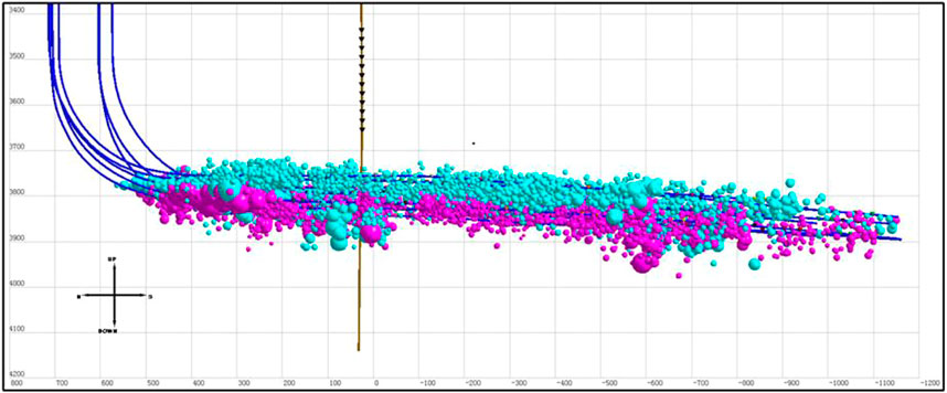
FIGURE 1. Microseismic monitoring map of well JL1.

Based on the fracture length and width obtained by on-site microseismic monitoring, the fracture complexity index can be preliminarily calculated (Cipolla et al., 2008), and the calculation result is used as the target value in the machine learning. The accuracy of the GEP calculation model is determined by the sample size and the selection of the geological engineering parameters that affect the fracture complexity index. By collecting the data of a total of 118 fracturing sections of 8 fracturing wells on site, a total of 14 possible influencing factors are considered in each section as the data samples for modeling and calculation analysis in this paper, including fracturing engineering parameters such as displacement and operation pressure and reservoir geological parameters.

2.1 Data collection

A total of 118 fracture stages from 8 wells were obtained as a data set to calculate the complex index of the conglomerate. Each stage is used as a data sample. The input includes 14 variables (engineering parameters and geological parameters), and the output variable is the fracture complexity index value, so there are a total of 14 input variables and one output variable. The distribution of the dataset is described in Table 1. It can be seen that there are obvious differences in the data distribution (such as data range) of each variable.

TABLE 1

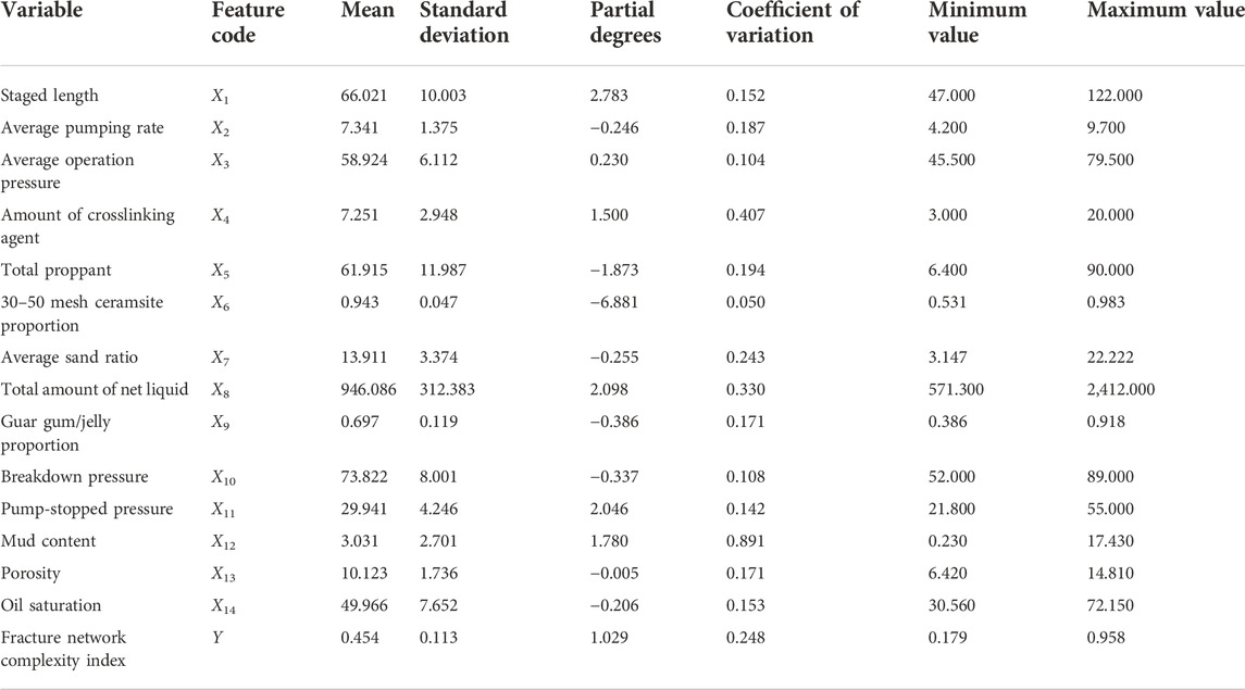
TABLE 1. Descriptive statistical table of characteristic parameters.

With different unit dimensions and data distribution, efficient machine learning models are sensitive to the distribution of features, so data preprocessing is important for machine learning. The data is moved by the minimum value unit, and will be converged to between [0,1], and it is called data normalization. The normalization formula (Qi et al., 2019) is:

$x*=\frac{x-\min \left(x\right)}{\max \left(x\right)-\min \left(x\right)}(1)$

where min(x) is the minimum value of data x; max(x) is the maximum value of data x; x* is the normalized value of data x.

2.2 Calculation and evaluation of basic data

2.2.1 Judgment of divergence

For the designed features, the coefficient of variation (C_V) is used to judge the degree of dispersion, which is defined as the ratio between the standard deviation of the feature and the mean value, and the expression is as follows:

$C_V=\frac{{\sigma }_X}{{\mu }_X}(2)$

After calculation, the results and ranking of the 14 feature dispersion coefficients designed are shown in Table 2. Generally speaking, the larger the dispersion coefficient C_V, the more dispersed the data are, and the more effective for prediction. It can be seen from Table 2 that the dispersion coefficient C_V of the five characteristics of mud content, amount of crosslinking agent, total amount of net liquid, average sand ratio, and total proppant are relatively large, and the values of the data are relatively scattered and strongly divergent.

TABLE 2

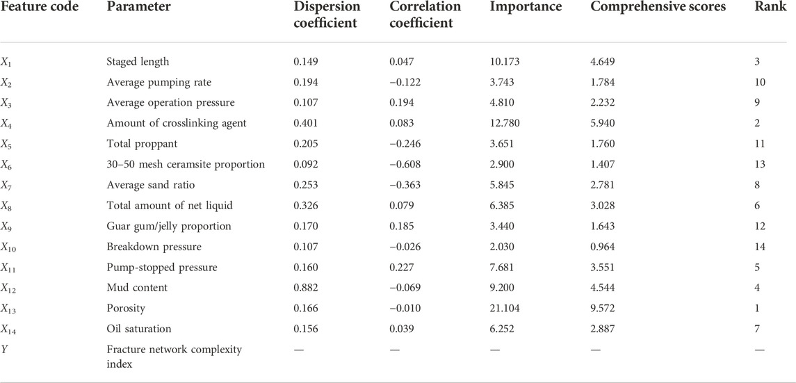
TABLE 2. Characteristic parameter calculation results.

2.2.2 Judgment of correlation

Pearson’s correlation coefficient (PCC) was used to judge the correlation between 14 features and fracture complexity index. PCC is a classical statistic used to reflect the degree of linear correlation between two variables. The correlation coefficient is represented by ρ_X,Y, which is the covariance cov(X,Y) of two variables X,Y divided by their standard deviations σ_X and σ_Y. The result is between -1 and 1, and the larger the absolute value of ρ, the stronger the correlation.

${\rho }_{X,Y}=\frac{\mathrm{c}\mathrm{o}\mathrm{v}\left(X,Y\right)}{{\sigma }_X\cdot {\sigma }_Y}=\frac{{\displaystyle \sum }_{i=1}^n\left(X_i-\overline{X}\right)\left(Y_i-\overline{Y}\right)}{\sqrt{{{\displaystyle \sum }_{i=1}^n\left(X_i-\overline{X}\right)}^2}\sqrt{{{\displaystyle \sum }_{i=1}^n\left(Y_i-\overline{Y}\right)}^2}}(3)$

where X is feature; Y is predictor variable; σ_x is the standard deviation of X; σ_Y is the standard deviation of Y.

The pearson correlation coefficient between the characteristics and the calculated value of fracture complexity index is shown in Table 2.

2.2.3 Feature importance judgment

Random forest is a classic ensemble model based on bagging to improve the performance of basic decision tree models. CatBoost is a parallel computing model based on boosting to gradually iterate decision tree models to improve the fitting effect (BuKhamseen et al., 2017). The CatBoost model is selected for importance judgment in this paper. After the training of the CatBoost model, the relative importance score of each feature is directly output by the model. The importance of the fracture complex index is shown in Table 2.

2.2.4 Feature synthesis calculation

Regarding the correlation between the feature and the complexity index, a weighted evaluation of the three evaluation indexes (the sum of the weights is 1) is defined. A comprehensive fracture complexity index correlation is given to the feature score by integrating the results of different evaluation methods. The C_V score reflects the divergence of the feature, that is, the amount of information. A weight of 0.1 is assigned to the C_V score (w₃), the remaining weights are equally distributed to PCC and CatBoost. The comprehensive scores are shown in Table 2.

$Score=w_1\cdot S_{\mathrm{P}\mathrm{C}\mathrm{C}}+w_2\cdot S_{\mathrm{C}\mathrm{a}\mathrm{t}\mathrm{B}\mathrm{o}\mathrm{o}\mathrm{s}\mathrm{t}}+w_2\cdot S_{\mathrm{C}\mathrm{V}}(4)$

2.2.5 Independent judgment

There is not only a correlation between the feature and the fracture complex index, but also a correlation within the feature, that is, between the input variables. The correlation between the 14 input variables is judged by the PCC. As shown in Figure 2A, some of the correlation coefficients are greater than 0.5, indicating that there is a strong correlation between the input variables (Koo et al., 2016). Strong correlation will make GEP biased in variable selection during training and prediction, resulting in poor model correlation. Therefore, it is necessary to combine the importance and independence of features to re-divide the features, and the poor independence features are classified into one category. The selection can not only reflect the important factors, but also ensure the independence between features and improve the accuracy of the model. Based on the comprehensive score of features, the important factors are first selected and then classified according to their independence. The classification results are shown in Table 3 and the reconstructed features are F₁∼F₁₀. The importance distribution histogram are shown in Figure 2B.

FIGURE 2

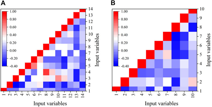
FIGURE 2. Independence among 14 variables (A) and 10 reconstructed variables (B).

TABLE 3

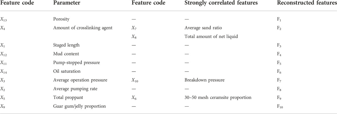
TABLE 3. Reconstruction feature parameter correspondence table.

2.2.6 Principal component analysis

Some strongly correlated variables can be excluded and features that carry important information can be selected by judging the importance and independence of the features above. All the information that affects the complex index is carried in the remaining reconstructed features (F₁∼F₁₀), but it is inevitable that there will be poor independence between the reconstructed features, which will cause some information to be ignored or covered. And then the accuracy and generalization ability of the GEP calculation model will seriously be affected. Therefore, the principal component analysis method (Sircar et al., 2021) is used to eliminate the weak independence between the reconstructed variables. The input reconstruction features are recombined into a new set of mutually unrelated variables, while retaining the information carried by the original variables. After the dealing with PCA, the correlation between the variables is shown in Figure 3. It can be seen that the variables are independent of each other, and the GEP model can be trained after the PCA processing.

FIGURE 3

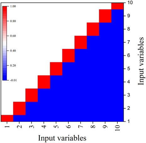
FIGURE 3. Independence among 10 variables after PCA processing.

2.3 Gene expression programming

2.3.1 GEP principle

The evolutionary algorithm is a method to search for the maximum or minimum value of a function by simulating Darwin’s evolutionary theory of the survival of the fittest in natural organisms. It is suitable for solving complex problems and is used in various fields. The model has strong robustness and is especially suitable for establishing complex functional relationships between variables. Compared with other machine learning algorithms (such as random forests, neural networks, etc.), evolutionary algorithms are interpretable. The advantages of GA and GP are inheritted by GEP, expressing structures of different sizes and shapes using simple, linear, fixed-length individuals. The main genetic operators used in GEP include mutation, inversion, transposition, crossover/recombination, and gene crossover (Ferreira, 2001).

2.3.2 Assessment of the results

To evaluate the performance of the trained GEP model, a statistical index is introduced, which is the mean squared error(RMSE) (Emamgolizadeh et al., 2015). It is used to describe the difference between the model calculated value and the field actual value, which is shown in Eq. 5. The smaller the RMSE, the better the performance of the model.

$RMSE=\sqrt{\frac{1}{n}{{\displaystyle \sum }_{i=1}^n\left(y_i-Y_i\right)}^2}(5)$

where Y_i is fracture complex index value obtained in field, dimensionless; y_i is predicted fracture complexity index value, dimensionless; Y is fracture complex index mean value obtained in field, dimensionless; y is predicted fracture complexity index mean value, dimensionless; n is the number of data samples, dimensionless.

2.3.3 Fitness function

If the chosen error is the absolute error, the fitness f_i of a single program i is calculated by Eq. 6. If the selected error is a relative error, then the Eq. 7 is used to calculate this value.

$f_i={\displaystyle \sum }_{C_i}^{j=1}\left(M-\left|C_{\left(i,j\right)}-T_{\left(j\right)}\right|\right)(6)$

$f_i={\displaystyle \sum }_{C_i}^{j=1}\left(M-\left|\frac{C_{\left(i,j\right)}-T_{\left(j\right)}}{T_{\left(i\right)}}\cdot 100\right|\right)(7)$

where M is the selection range, C_(i,j) is the value returned by individual chromosome i for fitness case j (outside of C_t fitness case), and T_j is the target value for fitness case j. Note that for full adaptation, C_(i,j) = T_j, f_i = f_max = C_t·M。

2.3.4 GEP algorithm flow

Combined with the principle of the GEP algorithm, the GEP evolution process is shown in Figure 4.

FIGURE 4

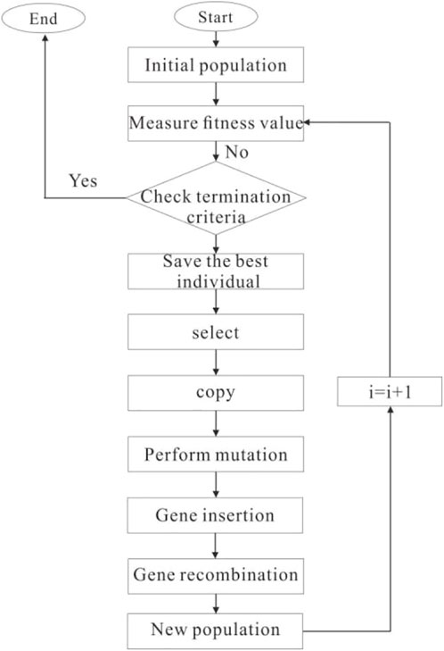
FIGURE 4. Flow chart of GEP evolution.

3 Applications and analysis

At present, there are many studies on the selection of training set and test set size in machine learning. Generally, 70% is selected as the train set size (Qi et al., 2018). Therefore, the data of 83 fracturing stages is selected as training set samples, and the remaining 35 stages are used as test set samples for GEP fitting.

3.1 Fitting of equations

The accuracy and validity of the GEP model depend on many factors. Whether the input variables are independent of each other plays an important role in the selection of important variables during equation fitting. Therefore, the reconstruction variables (F₁, F₂, F₃...F₁₀) are used as the input variables of the GEP model to calculate the fracture complex index of the sandy conglomerate reservoir based on the previous analysis. In this study, basic operators such as +、-、∗、/、exp、Inv、Min、Max are used to implement the GEP model. The fitted equation is shown in Eq. 8, in which y₁∼y₁₀ are shown in Eq. 9, and the equation coefficients are shown in Table 4.

$y=y_1+y_2+y_3+y_4+y_5+y_6+y_7+y_8+y_9+y_{10}(8)$

$\left\{\begin{array}{l}{y}_1=\left(x_{10}*\left(\max \left({\mathrm{a}}_4,gep\left(\max \left({\mathrm{a}}_3,{\mathrm{a}}_2\right)\right)\right)-e^{\left(x_1*{\mathrm{a}}_1+\max \left(x_4,x_1\right)\right)/2}\right)+\left(gep\left(\left({\mathrm{a}}_4-x_3\right)*\left(x_8-x_{10}\right)*x_8*x_6\right)*x_2\right)\right)/2\\ y_2=x_9^2/\left(\left(\left({\left(x_8*{\mathrm{b}}_1*gep\left({\mathrm{b}}_1\right)\right)}^2+{\mathrm{b}}_1*x_1\right)/2\right)-\left(\left(\left({\mathrm{b}}_2^2+{\mathrm{b}}_2+x_3\right)/2\right)-x_2\right)*x_{10}^2\right)\\ y_3=(\left(\left(1/\left(\left(\left(\left(\left(1-\left(\left(\left({\mathrm{c}}_1-x_6\right)*x_2*x_6+\left(x_7+{\mathrm{c}}_2\right)/2\right)/2\right)\right)+\left(x_{10}+x_1/2)\right)\right)+(x_6+x_7)/2)\right)\right)\right)*x_7\right)+\left(1-x_3\right)\right)/2\\ y_4=x_9-\left(x_9-\min (x_{10},\left(\left(\left(1-\left({\left(\left(\left((\left(x_4+x_{10}\right)+({\mathrm{d}}_2+x_4)/2/2)+\left({\mathrm{d}}_1*x_1\right)/2\right)-\min \left(\left(x_6+{\mathrm{d}}_1\right),\left(x_3+x_5\right)/2\right)\right)\right)}^2+x_9\right)/2\right)\right)\right)\right)\\ y_5=2*x_9*e^{{\left(\left(\left(\left(x_4-x_6\right)*{\mathrm{e}}_2+\left(x_1+{\mathrm{e}}_1\right)/2\right)/2+\left(1\text{-}{x}_9\right)/2\right)\right)}^2}*\min \left(x_4,\left(1-gep\left(1-\left(x_{10}-x_1\right)\right)\right)\right)\\ y_6=x_1*gep\left(\left(\left(\left(\left({\mathrm{f}}_1*x_{10}-{\mathrm{f}}_3\right)*\left({\mathrm{f}}_2+x_7\right)/2\right)+x_{10}/x_8\right)/2*\max \left(x_3,{\left(x_1*x_2\right)}^2\right)\right)-x9)*x_3\right),\\ y_7=\min \left(\left(x_3-2*x_6^2*\left(1/\left(\left(\left(\left({\mathrm{g}}_1+x_6\right)+x_6\right)+{\mathrm{g}}_2+x_5\right)+\left(x_3^2+x_7/x_6\right)\right)\right)\right),{\mathrm{g}}_3\right)\\ y_8=x_8\\ y_9=((\left(1-x_3\right)*x_{10}*(gep\left({\mathrm{h}}_1*x_3\right)\ast e^{{\mathrm{h}}_2}/(\left(1-{\mathrm{h}}_3\right)-1/x_{10})-x_{10})*e^{x_6})+x_{10})/2\\ y_{10}=\min \left(\left(\left(\left(\left(1-x_3\right)+2*x_9\right)+1/\left(1-x_7\right)\right)-\left(2*x_{10}+x_2^2\right)\right)+\left({\mathrm{k}}_2+x_2\right)/2*x_5*{\mathrm{k}}_3/gep\left(\left({\mathrm{k}}_1+x_9\right)/2\right),x_9\right)\end{array}\right.(9)$

$gep\left(x\right)=\left\{\begin{array}{ll}-{\left(-x\right)}^{\frac{1}{3}}& ,x<0\\ x^{\frac{1}{3}}& ,x>0\end{array}\right.(10)$

TABLE 4

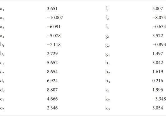
TABLE 4. Equation coefficient table.

3.2 Result analysis

According to the obtained GEP model, the training and test set of fracture complex index are analyzed. In order to get a clearer understanding of the accuracy and reliability of the model, a comparison chart of the fracture complexity index and data point sequence of the actual field results and the model calculation results is also drawn, as shown in Figure 5. It demonstrates the accuracy of the developed model and the GEP model correctly calculate the trend of the field data by comparing the target value and the calculated value in the training and test set.

FIGURE 5

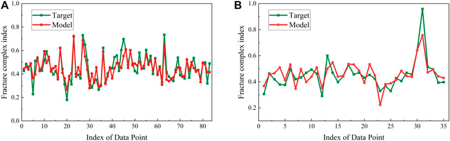
FIGURE 5. Simultaneous plot of outcomes of the GEP model and target data against index of data: (A) training set and (B) test set.

The fracture complexity index values from actual field data and the calculated results is compared in the Figure 6. It can be seen that the GEP model successfully learns the relationship between the nonlinear fracture complexity index and its influencing variables. The data points are mainly distributed around the diagonal, implying that there is a proper coordination between the calculated data and the target data. Computational performance is evaluated using R and RMSE, and in the case of the training set, the statistical parameters obtained by GEP are: R=0.861, RMSE=0.058. According to statistical suggestions, when R>0.8, it means that the calculation result is better (Roy et al., 2008). Therefore, the computational performance of GEP is satisfactory in the training set. Likewise, the statistical parameters of the test set are: R=0.817 and RMSE=0.066, indicating that the model trained by GEP can be used to calculate the fracture complexity index.

FIGURE 6

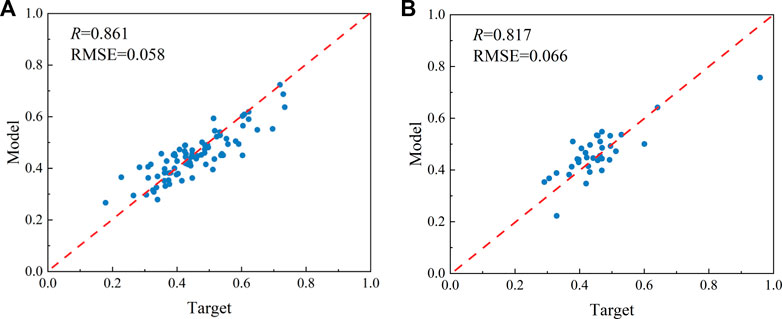
FIGURE 6. Comparison of target value of fracture complexity index and calculated value of GEP model: (A) training set and (B) test set.

In order to analyze the influencing factors of the fracture complex index, the Permutation Importance (PI) method was used to determine the importance of the factors. It provides a model-independent method for calculating feature importance by selecting a feature and using the test set to calculate a score (standard deviation). Randomly shuffle the values of the feature column of the test set, and calculate the score (standard deviation) of the feature. The effect of the feature on the calculation can be obtained by taking the difference of the score, and then the effect of each feature on the calculation can be obtained. If there is little difference between the old and new results, it means that the feature is of low importance. If the difference between them is significant, then the effect on the model is also significant. Finally, the scores of all features are ranked to get the importance.

The relative importance of the feature variables to the fracture complexity index calculated using the feature importance evaluation method PI is shown in Table 5. Among them, the more important engineering control factors are the ratio of guar gum/jelly, the amount of crosslinking agent and the pump stop pressure, etc. And the more important geological control factor is the mud content.

TABLE 5

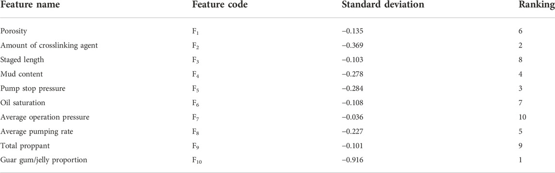
TABLE 5. The ranking of main control factors.

4 Discussion

Two important issues are discussed in this section. The first is to analyze how the controlling factors, such as geological parameters and engineering parameters, affect the fracture complexity index by using the model. The second is whether the model trained using GEP can be used to calculate the fracture complex index.

The Partial Dependency Plot (PDP) shows the marginal effect of a feature on the results of a previously fitted model calculation, reflecting how this feature affects the calculation. To obtain a partial correlogram (Friedman, 2001), several values of the input variable are first selected, and then, for all cases of the other input variables, each of these values is used to calculate the output. Finally, the average output is calculated and then compared with the corresponding input value. And the partial dependence relationship between some important engineering and geological parameters in the reconstruction variables and the fracture complex index is drawn as shown in the figures.

It can be seen from Figure 7 that the engineering parameters have different degrees of influence on the fracture complexity index. According to the PI calculation results, the proportion of guar gum/jelly is an important controlling factor. With the increase of the proportion, the fracture complex index shows an upward trend, but when the proportion of guar gum/jelly is about 70%, the fracture complexity index begins to decrease. The increasing of the proportion can effectively promote the net pressure in the fracture, which is beneficial to form complex fractures. In addition, with the increase of the crosslinking agent, the fracture complexity index first increases and then decreases, and there is an optimal value.

FIGURE 7

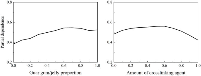
FIGURE 7. Partial dependency plot of engineering parameters(A) of GEP model.

It can be seen from Figure 8 that the fracture complexity index increases with the increase of the pump-stop pressure, and the higher the pump-stop pressure, the higher the net pressure in the fracture, which can significantly promote the fracture complexity. At the same time, it can be seen that the fracture complexity index increases first and then decreases with the variety of the fracturing stage length, indicating that when the fracturing stage is short, although the length of the stage is fully stimulated, the stimulated area has a low degree of fracture complexity. When the fracturing stage is long, it may not be completely stimulated, the fracture width of microseismic monitoring is smaller than the fracturing stage length, and the fracture complexity is still small. The optimal fracture complexity can be obtained while the fracture length is extended, the lateral stimulated degree is maximized, and the fracture width monitored is approximately equal to the stage length after fracturing by optimizing a reasonable stage length.

FIGURE 8

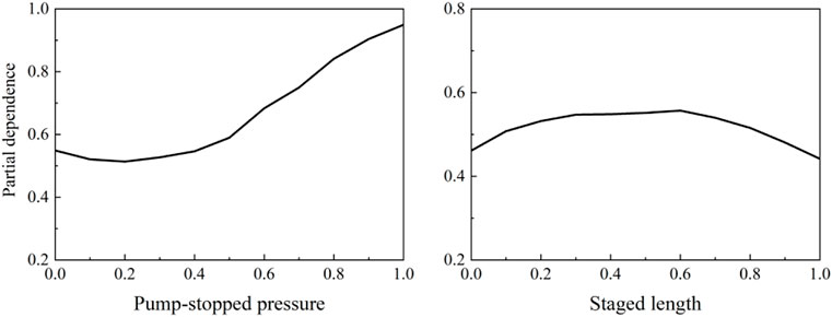
FIGURE 8. Partial dependency plot of engineering parameters(B) of GEP model.

Whether the hydraulic fracture can be effectively supported depends to a large extent on the proppant. The selection of proppant specifications is mainly based on the comprehensive consideration of formation sand feeding capacity, proppant conductivity, and proppant breakage rate under the closing stress condition of the target layer. The 30/50 mesh ceramsite and 40/70 mesh quartz sand is used, and it can be seen from the Figure 9 that the amount of proppant within a certain range can promote the formation of complex fractures, and the proppant with small particle size can play the role of temporary blocking and turning.

FIGURE 9

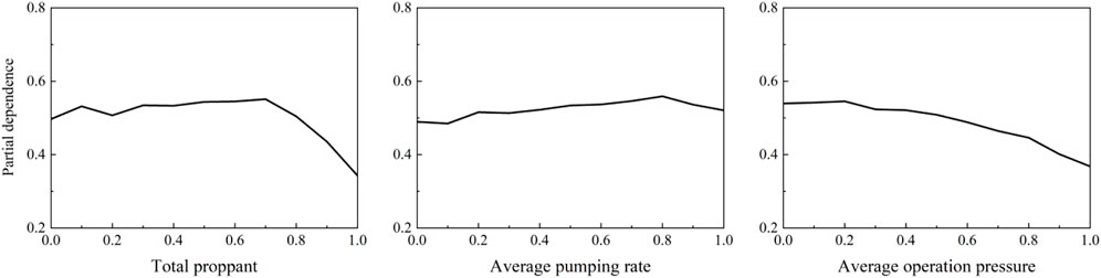
FIGURE 9. Partial dependency plot of engineering parameters(C) of GEP model.

The practice of hydraulic fracturing shows that the larger the pumping rate, the greater the net pressure, which is Figure 9 conducive to the propagation of hydraulic fractures. However, the sandy conglomerate reservoir is different from the shale and other natural fracture-developed reservoirs, so the effect of increasing the pumping rate on the fracture complexity index is relatively slow.

The operation pressure is predicted under different pumping rate, considering the need for full stimulation of a single cluster. There are 2 clusters in a single stage, each cluster is 1 m/16 holes, a total of 32 holes, when the pumping rate is 8∼10 m³/min, the predicted operation pressure is 56∼59 MPa. The average pumping rate is 4.2∼9.7 m³/min in this paper. Therefore, the pumping rate within this range will not lead to excessive operation pressure. Different from the pump stop pressure, the operation pressure shows the opposite trend. Before fracturing, the operation pressure limit at different sand concentration can be calculated to ensure the safe operation. When the operation pressure varies greatly, it is difficult for the hydraulic fracture to propagate, resulting in a low fracture complexity index.

As shown in Figure 10, for low-porosity sandy conglomerate reservoirs, the fracture complexity index shows an upward trend, which is related to the high elastic characteristics of low-porosity rocks. For high-porosity sandy conglomerate reservoirs, the effect of porosity on the fracture complexity index can be ignored. In the range of mud content in the target block, the effect on the complexity is low. Under low oil saturation, the fracture complex index can be improved due to the small content of pore-liquid phase and strong rock elastic characteristics. When the oil saturation is too high, the complex index is suppressed.

FIGURE 10

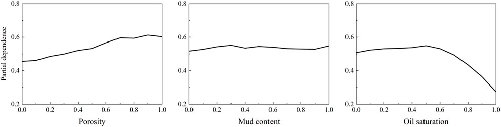
FIGURE 10. Partial dependence plot of geological parameters of GEP model.

In general, the above discussion shows that the trained calculation model can be used for the calculation and characterization of fracture complex index in this area to achieve better results.

5 Conclusion

(1) Based on the internal relationship between reservoir geoengineering parameters and fracture complexity index, the data of 118 fracturing stages in Jinlong Oilfield were collected. The Genetic Expression Programming (GEP) method, which has extensive advantages in solving multi-factor nonlinear fitting was introduced. And then a hydraulic fracture complex index calculation model was developed. It showed that the model can be extended to calculate the fracture complex index in sandy conglomerate reservoirs.

(2) The controlling factors affecting the fracture complex index were obtained, and the influence on the fracture complex index was analyzed by the partial dependence plot (PDP). It is found that engineering parameters have a greater impact on the fluctuation of the fracture complex index, followed by geological parameters. The influence law of the factors on fracture complex index was obtained in the sandy conglomerate.

(3) The intelligent method is a useful tool for solving complex mechanism problems, especially in the process of hydraulic fracturing. The fracture complex index calculation model established in this paper can be used to analyze the influencing factors of the sandy conglomerate reservoir in Jinlong Oilfield.

Data availability statement

The data analyzed in this study is subject to the following licenses/restrictions: The data comes from the actual data on site, which is confidential. Requests to access these datasets should be directed to WZ, wzh_swpu@126.com.

Author contributions

ZL: Conceptualization, methodology, design. WZ: Software, methodology, analysis. XR: Data collecting, reviewing and editing. CH: Writing—original draft preparation, revision. RL: Writing, validation, design. LR: Visualization, investigation.

Conflict of interest

Authors ZL, XR, and CH were employed by the company China National Petroleum Corporation.

The remaining authors declare that the research was conducted in the absence of any commercial or financial relationships that could be construed as a potential conflict of interest.

Publisher’s note

All claims expressed in this article are solely those of the authors and do not necessarily represent those of their affiliated organizations, or those of the publisher, the editors and the reviewers. Any product that may be evaluated in this article, or claim that may be made by its manufacturer, is not guaranteed or endorsed by the publisher.

References

Akolekar, H. D., Weatheritt, J., Hutchins, N., Sandberg, R. D., Laskowski, G., and Michelassi, V. (2019). Development and use of machine-learnt algebraic Reynolds stress models for enhanced prediction of wake mixing in low-pressure turbines. J. Turbomach. 141 (4), 041010. doi:10.1115/1.4041753

CrossRef Full Text | Google Scholar

BuKhamseen, N. Y., and Ertekin, T. (2017). Validating hydraulic fracturing properties in reservoir simulation using artificial neural networks. SPE. 9 188093.

CrossRef Full Text | Google Scholar

Cheng, B., Li, J., Li, J., Su, H., Tang, L., Yu, F., et al. (2022). Pore-scale formation damage caused by fracturing fluids in low-permeability sandy conglomerate reservoirs. J. Petroleum Sci. Eng. 208, 109301. doi:10.1016/j.petrol.2021.109301

CrossRef Full Text | Google Scholar

Cipolla, C. L., Warpinski, N. R., and Mayerhofer, M. J., The relationship between fracture complexity, reservoir properties, and fracture treatment design, SPE annual technical conference and exhibition, 2008. Denver, Colorado, USA, 21–24. doi:10.2118/115769-MS

CrossRef Full Text | Google Scholar

Emamgolizadeh, S., Bateni, S. M., Shahsavani, D., Ashrafi, T., and Ghorbani, H. (2015). Estimation of soil cation exchange capacity using genetic expression programming (GEP) and multivariate adaptive regression splines (MARS). J. Hydrology 529, 1590–1600. doi:10.1016/j.jhydrol.2015.08.025

CrossRef Full Text | Google Scholar

Ferreira, C. (2001). Gene expression programming: A new adaptive algorithm for solving problems. Complex Syst. 13 (2), 87–129.

Google Scholar

Friedman, J. H. (2001). Greedy function approximation: A gradient boosting machine. Ann. statistics, 43 1189–1232.

CrossRef Full Text | Google Scholar

Fu, H., Cai, B., Xiu, N., Wang, X., Liang, T., Liu, Y., et al. (2021). The study of hydraulic fracture vertical propagation in unconventional reservoir with beddings and field monitoring. Nat. Gas. Geosci. 32 (11), 1610–1621 (Chinese).

Google Scholar

Guo, J. (2019). Optimization design of volume fracturing parameters of horizontal wells in mahu glutenite reservoir. Beijing, china: China University of Petroleum.

Google Scholar

Guoxin, L. I., Jianhua, Q. I. N., Chenggang, X., Fan, X., Zhang, J., and Ding, Y. (2020). Theoretical understandings, key technologies and practices of tight conglomerate oilfield efficient development: A case study of the mahu oilfield, Junggar Basin, NW China. Petroleum Explor. Dev. 47 (6), 1275–1290. doi:10.1016/s1876-3804(20)60135-0

CrossRef Full Text | Google Scholar

Koo, T. K., and Li, M. Y. (2016). A guideline of selecting and reporting intraclass correlation coefficients for reliability research. J. Chiropr. Med. 15, 155–163. doi:10.1016/j.jcm.2016.02.012

PubMed Abstract | CrossRef Full Text | Google Scholar

Qi, C., Fourie, A., Ma, G., and Tang, X. (2018). A hybrid method for improved stability prediction in construction projects: A case study of stope hangingwall stability. Appl. Soft Comput. 71, 649–658. doi:10.1016/j.asoc.2018.07.035

CrossRef Full Text | Google Scholar

Qi, C., Tang, X., Dong, X., Chen, Q., Fourie, A., and Liu, E. (2019). Towards intelligent mining for backfill: A genetic programming-based method for strength forecasting of cemented paste backfill. Miner. Eng. 133, 69–79. doi:10.1016/j.mineng.2019.01.004

CrossRef Full Text | Google Scholar

Ren, L., Lin, R., Zhao, J., Rasouli, V., and Yang, H. (2018). Stimulated reservoir volume estimation for shale gas fracturing: Mechanism and modeling approach. J. Petroleum Sci. Eng. 166, 290–304. doi:10.1016/j.petrol.2018.03.041

CrossRef Full Text | Google Scholar

Ren, L., Lin, R., Zhao, J., and Wu, L. (2017). An optimal design of cluster spacing intervals for staged fracturing in horizontal shale gas wells based on the optimal SRVs. Nat. Gas. Ind. B 4 (5), 364–373. doi:10.1016/j.ngib.2017.10.001

CrossRef Full Text | Google Scholar

Ren, L., Wang, Z., Zhao, J., Wu, J., Lin, R., Wu, J., et al. (2022). Shale gas load recovery modeling and analysis after hydraulic fracturing based on genetic expression programming: A case study of southern sichuan basin shale. J. Nat. Gas Sci. Eng. 107, 104778. doi:10.1016/j.jngse.2022.104778

CrossRef Full Text | Google Scholar

Roy, P. P., and Roy, K. (2008). On some aspects of variable selection for partial least squares regression models. QSAR Comb. Sci. 27 (3), 302–313. doi:10.1002/qsar.200710043

CrossRef Full Text | Google Scholar

Shentu, J., Lin, B., Dong, J., Yu, H., Shi, S., and Ma, J., (2019).Investigation of hydraulic fracture propagation in conglomerate reservoirs using discrete element method, ARMA-CUPB Geothermal International Conference. Washington, DC, USA. ARMA-CUPB-19-7769.

Google Scholar

Sircar, A., Yadav, K., Rayavarapu, K., Bist, N., and Oza, H. (2021). Application of machine learning and artificial intelligence in oil and gas industry. Petroleum Res. 6, 379–391. doi:10.1016/j.ptlrs.2021.05.009

CrossRef Full Text | Google Scholar

Wang, S., Qin, C., Feng, Q., Javadpour, F., and Rui, Z. (2021). A framework for predicting the production performance of unconventional resources using deep learning. Appl. Energy 295, 117016. doi:10.1016/j.apenergy.2021.117016

CrossRef Full Text | Google Scholar

Wang, S., Wang, X., Bao, L., Feng, Q., and Xu, S. (2020). Characterization of hydraulic fracture propagation in tight formations: A fractal perspective. J. Petroleum Sci. Eng. 195, 107871. doi:10.1016/j.petrol.2020.107871

CrossRef Full Text | Google Scholar

Weatheritt, J., and Sandberg, R. D. (2017). The development of algebraic stress models using a novel evolutionary algorithm. Int. J. Heat Fluid Flow 68, 298–318. doi:10.1016/j.ijheatfluidflow.2017.09.017

CrossRef Full Text | Google Scholar

Wen, Q., Zhang, J., and Li, M. (2015). A new correlation to predict fracture pressure loss and to assist fracture modeling in sandy conglomerate reservoirs. J. Nat. Gas Sci. Eng. 26, 1673–1682. doi:10.1016/j.jngse.2015.04.007

CrossRef Full Text | Google Scholar

Xv, C. Z., Zhang, G. Q., Lyu, Y. J., Xv, Q. S., et al. (2020). The influence of gravels on hydraulic fracture propagation of conglomerate, Rock Mechanics/Geomechanics Symposium. Washington, DC, USA. ARMA-2020-1644.

Google Scholar

Xv, C., Zhang, G., Yanjun, L., Wang, P., et al. (2019). Experimental study on hydraulic fracture propagation in conglomerate reservoirs, Rock Mechanics/Geomechanics Symposium. Washington, DC, USA. ARMA-2019-1844.

Google Scholar

Yushi, Z. O. U., Shanzhi, S. H. I., Zhang, S., Yu, T., Tian, G., Ma, X., et al. (2021). Experimental modeling of sanding fracturing and conductivity of propped fractures in conglomerate: A case study of tight conglomerate of mahu sag in Junggar Basin, NW China. Petroleum Explor. Dev. 48 (6), 1383–1392. doi:10.1016/s1876-3804(21)60294-x

CrossRef Full Text | Google Scholar

Zhao, J., Ren, L., Jiang, T., Hu, D., Wu, L., Wu, J., et al. (2022). Ten years of gas shale fracturing in China: Review and prospect. Nat. Gas. Ind. B, 9, 158, 175, doi:10.1016/j.ngib.2022.03.002

CrossRef Full Text | Google Scholar

Zhao, J., Ren, L., Shen, C., and Li, Y. (2018). Latest research progresses in network fracturing theories and technologies for shale gas reservoirs. Nat. Gas. Ind. B 5 (5), 533–546. doi:10.1016/j.ngib.2018.03.007

CrossRef Full Text | Google Scholar