Spatial averaging implied in aquifer test interpretation: The meaning of estimated hydraulic properties

1 Introduction

Aquifer tests comprise an essential component of site characterisation studies. A well is pumped, often at a constant rate, for a certain amount of time. Drawdowns are measured in the pumped well and possibly in one or a number of observation wells. Local hydraulic properties are inferred from these drawdowns.

Interpretation of aquifer test data is generally based on a number of simplifying assumptions. In the simplest case, the pumping well is assumed to fully penetrate a confined aquifer. The aquifer is imagined to be homogeneous; groundwater flow that is induced by pumping is therefore presumed to be radial.

Under these circumstances, drawdown can be calculated using the Theis equation (Theis 1935). Back-calculation of aquifer transmissivity (T) and storativity (S) can therefore be achieved by finding values of T and S for which the Theis curve provides the best fit with observed drawdowns. This can be done manually, or it can be automated. Where drawdowns are measured in a number of observation wells, it is commonplace to subject each set of well-specific drawdowns to this kind of analysis. While values inferred for T and S may differ between wells, all of them are reported. Differences between them are taken as a measure of local hydraulic property heterogeneity.

The Theis assumption of hydraulic property homogeneity over the entire drawdown-affected area can rarely be justified. It is made in order to attain uniqueness of an inverse problem, and to permit use of a simplified forward model for computation of drawdown. It is presumed that solution of this simplified inverse problem yields values of T and S that are “representative” of the area in which drawdown has been induced.

A number of authors have inquired into the nature of the relationship between real and inferred hydraulic properties. These include Butler (1988), Butler (1990), Oliver (1990), Oliver (1993), Sánchez-Vila, et al. (1999), Leven and Dietrich (2006) and Copty et al. (2011). Most of these studies focussed on the relationship between drawdown in a pumped or observation well and hydraulic properties that characterise pumping-affected areas. Linearization of this relationship enables rapid evaluation of drawdown-to-parameter sensitivities. It is argued that greater sensitivity of drawdown to hydraulic properties that prevail in one area over those that prevail in another area implies that values of T and S that are inferred from these drawdowns are more reflective of properties in the former area than those in the latter area.

In this paper we extend the utility of linear analysis in order to derive equations that directly relate values for T and S that are forthcoming from Theis-based analysis of drawdowns to values of T and S that characterise an aquifer; the former are referred to as “apparent values” by Sanchez-Vila et al. (2006). The methodology that we employ can be readily extended to other aquifer test contexts where forward modelling of pumping-induced drawdown relies on fewer assumptions than those that are required by the Theis equation. However, linear analysis under Theis assumptions is rendered particularly easy by the availability of analytical formulae for calculation of drawdown-to-parameter sensitivities.

2 Theory

2.1 Fréchet kernels

Consider a pumping well situated at (−a/2, 0) and an observation well at (a/2, 0); they are separated by a distance a. At time zero, extraction of water begins at a rate of q₀. The situation is depicted in Figure 1.

FIGURE 1

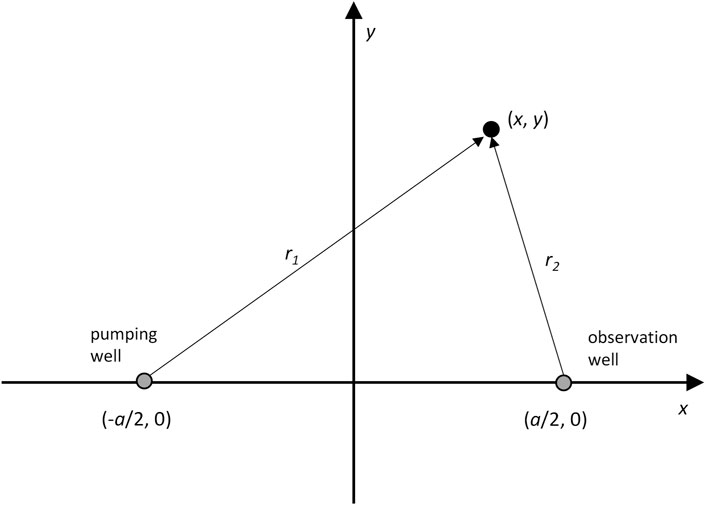
FIGURE 1. A pumping and observation well. Also shown is a general point in two-dimensional space. The hydraulic properties at this point are functions of location (x, y).

Suppose that the medium which these wells penetrate is homogeneous, with a pervasive transmissivity of T₀ and a pervasive storativity of S₀. Under these circumstances, drawdown s at the observation well can be calculated using the Theis equation:

$s\left(\frac{a}{2},t\right)=\frac{q_0}{4\pi T_0}{E}_1\left(\frac{S_0{a}^2}{4T_{0}t}\right)(1)$

where E₁ is the exponential integral function.

Now suppose that the aquifer test host medium is not homogeneous, and that transmissivity and storativity are functions of location x i.e. (x, y). We further suppose that heterogeneities in transmissivity and storativity can be viewed as perturbations of background T_o and S_o. We denote differences between actual and background transmissivity and storativity by T and S. That is:

$T\left(\mathit{x}\right)=T_a\left(\mathit{x}\right)-T_0(\mathrm{2a})$

$S\left(\mathit{x}\right)=S_a\left(\mathit{x}\right)-S_0(\mathrm{2b})$

where T_a(x) and S_a(x) are the actual values of transmissivity and storativity at location x. If T(x) and S(x) are small, then the drawdown perturbation h(t) at the pumping well arising from these hydraulic property perturbations can be formulated as a convolution integral as follows:

$h\left(t\right)=\underset{A}{{\displaystyle \int }}T\left(\mathit{x}\right)F_T\left(\mathit{x},t\right)d\mathit{x}+\underset{A}{{\displaystyle \int }}S\left(\mathit{x}\right)F_S\left(\mathit{x},t\right)d\mathit{x}(3)$

The functions F_T(x,t) and F_S(x,t) comprise so-called Fréchet kernels for transmissivity and storativity respectively. Knight and Kluitenberg (2005) derived the following analytical expressions for them:

$F_T\left(\mathit{x},t\right)=-\frac{q_0\left(r^2-a^2/4\right)}{8{\pi }^{2}D{T}_0^2{r}_1{r}_{2}t}{K}_1\left(\frac{r_1{r}_2}{2Dt}\right)\exp \left(-\frac{r^2+a^2/4}{2Dt}\right)(\mathrm{4a})$

$F_S\left(\mathit{x},t\right)=-\frac{q_0}{8{\pi }^2{T}_0^{2}t}{K}_0\left(\frac{r_1{r}_2}{2Dt}\right)\exp \left(-\frac{r^2+a^2/4}{2Dt}\right)(\mathrm{4b})$

In these equations K₀ and K₁ are modified Bessel functions of order 0 and 1, while:

$r=\sqrt{\left(x^2+y^2\right)}(5)$

and

$D=\frac{T_0}{S_0}(6)$

r₁ and r₂ are depicted in Figure 1. Similar equations were derived by Zha et al. (2020).

The sensitivities of observation well drawdown to domain-wide transmissivity and storativity are obtained by areal integration of the respective Fréchet kernels. From Knight and Kluitenberg:

$M_T\left(t\right)=\underset{-\infty }{\overset{\infty }{{\displaystyle \int }}}\underset{-\infty }{\overset{\infty }{{\displaystyle \int }}}{F}_T\left(\mathit{x},t\right)d\mathit{x}=-\frac{q_0}{4\pi T_0^2}\left[E_1\left(\frac{S_0{a}^2}{4T_{0}t}\right)-\exp \left(-\frac{S_0{a}^2}{4T_{0}t}\right)\right](\mathrm{7a})$

$M_s\left(t\right)=\underset{-\infty }{\overset{\infty }{{\displaystyle \int }}}\underset{-\infty }{\overset{\infty }{{\displaystyle \int }}}{F}_S\left(\mathit{x},t\right)d\mathit{x}=-\frac{q_0}{4\pi S_0{T}_0}\exp \left(-\frac{S_0{a}^2}{4T_{0}t}\right)(\mathrm{7b})$

In the Supplementary Material we show how Knight and Kluitenberg’s Fréchet kernels can be extended to accommodate the T_x and T_y components of directional transmissivity. The extended kernels are:

$F_{T_x}\left(\mathit{x},t\right)=-\frac{q_0\left(x+a/2\right)\left(x-a/2\right)}{8{\pi }^{2}D{T}_0^2{r}_1{r}_{2}t}{K}_1\left(\frac{r_1{r}_2}{2Dt}\right)\exp \left(-\frac{r^2+a^2/4}{2Dt}\right)(\mathrm{8a})$

$F_{T_y}\left(\mathit{x},t\right)=-\frac{q_0{y}^2}{8{\pi }^{2}D{T}_0^2{r}_1{r}_{2}t}{K}_1\left(\frac{r_1{r}_2}{2Dt}\right)\exp \left(-\frac{r^2+a^2/4}{2Dt}\right)(\mathrm{8b})$

Note that these sum to F_T(x,t). With T_x and T_y treated separately, Eq. 3 becomes:

$h\left(t\right)=\underset{A}{{\displaystyle \int }}{T}_x\left(\mathit{x}\right)F_{T_x}\left(\mathit{x},t\right)d\mathit{x}+\underset{A}{{\displaystyle \int }}{T}_y\left(\mathit{x}\right)F_{T_y}\left(\mathit{x},t\right)d\mathit{x}+\underset{A}{{\displaystyle \int }}S\left(\mathit{x}\right)F_S\left(\mathit{x},t\right)d\mathit{x}(9)$

2.2 Parameter estimation

Suppose that we wish to back-calculate transmissivity and storativity from drawdowns measured in an observation well. This comprises an ill-posed inverse problem as it is impossible to assign unique values of transmissivity and storativity to all drawdown-affected points within a heterogeneous aquifer. If uniqueness is sought, it must be attained through regularisation. In aquifer test analysis, regularisation is usually achieved by assuming hydraulic property uniformity. In the present case, this reduces inverse problem complexity to that of estimating just two parameters, namely those that represent the transmissivity and storativity of the entire medium. This simplifies the analysis considerably. Meanwhile, it is hoped that the values of domain-wide transmissivity and storativity that emerge from this process are not too different from the “average” transmissivity and storativity of the porous medium which hosts the pumping test. Shortly, we examine whether this hope is well-placed.

We continue to assume a linear relationship between drawdown and aquifer hydraulic properties. This is in accordance with the theory on which most parameter estimation methods are based. In practical parameter estimation, non-linearities in this relationship are accommodated through iterative updating of sensitivities as estimated parameter values change.

The matrix-vector equation on which linearized parameter estimation is based can be written as follows:

$\mathbf{h}=\mathbf{M}\mathbf{p}+\mathbf{\epsilon }(10)$

In Eq. 10 the h vector contains differences between measured drawdowns in the observation well and those that are calculated using the domain-wide background values T₀ and S₀. Let us suppose that there are n such drawdown measurements. The vector p contains adjustments T and S to T₀ and S₀ (Eqs 2a, 2b). That is:

$\mathbf{p}=\left[\begin{array}{c}T\\ S\end{array}\right](11)$

ε (another n-dimensional vector) encapsulates random noise that is associated with measurements of drawdown. The n × 2 matrix M can be written as follows:

$\mathbf{M}=\left[\begin{array}{cc}{M}_T\left(t_1\right)& M_S\left(t_1\right)\\ M_T\left(t_2\right)& M_S\left(t_2\right)\\ .& .\\ M_T\left(t_n\right)& M_S\left(t_n\right)\end{array}\right](12)$

where M_T(t_i) and M_S(t_i) are Eqs 7a, 7b calculated at time t_i.

The least squares solution to the inverse problem posed by Eq. 10 [see, for example, Draper and Smith (1998)] is:

${\mathbf{p}}_{-}={\mathbf{(M}}^{\mathbf{t}}{\mathbf{QM)}}^{\mathrm{-1}}{\mathbf{M}}^{\mathbf{t}}\mathbf{Qh}(13)$

where Q is an observation weight matrix. Ideally Q is proportional to the inverse of the covariance matrix of measurement noise C(ε). The latter is normally assumed to be diagonal; so too is Q.

The elements of h can be calculated from distributed transmissivity and storativity using Eq. 3 or Eq. 9. The choice depends on whether or not we wish to characterise transmissivity using T alone, or T_x and T_y separately. To reduce complexity of the following equations, we first consider T on its own.

Equation 3 can be written in vector form as:

$\mathbf{h}=\mathbf{F}\mathbf{k}.(14)$

where k is the vector:

$\mathbf{k}=\left[\begin{array}{c}{T}_1\\ .\\ T_m\\ S_1\\ .\\ S_m\end{array}\right](15)$

The subscripts that accompany T and S in the k vector of Eq. 15 signify discretisation of x-y space into m elements (where m is a large number) for the purpose of numerical integration. In the present study we employ equal-sized, square cells and apply the midpoint rule.

To specify the F matrix, we write the integrals in Eq. 3 as summations:

$h_i={\displaystyle \sum }_A{F}_{i,j}^T{T}_j+{\displaystyle \sum }_A{F}_{i,j}^S{S}_j(16)$

where i denotes the i’th time at which drawdown measurements were made, and j denotes the j’th cell that is used for spatial integration. With k defined by Eq. 15, F becomes:

$\mathbf{F}=\left[\begin{array}{cccccc}{F}_{\mathrm{1,1}}^T& & F_{1,m}^T& F_{\mathrm{1,1}}^S& & F_{1,m}^S\\ & & & & & \\ F_{n,1}^T& & F_{n,m}^T& F_{n,1}^S& & F_{n,m}^S\end{array}\right](17)$

We now substitute Eq. 14 into Eq. 13 to obtain:

${\mathbf{p}}_{-}={\mathbf{(M}}^{\mathbf{t}}{\mathbf{QM)}}^{\mathrm{-1}}{\mathbf{M}}^{\mathbf{t}}\mathbf{Fk}(18)$

This can be re-written as:

${\mathbf{p}}_{-}=\mathbf{R}\mathbf{\prime }\mathbf{k}(19)$

where R′ is defined through this equation.

The matrix R′ has two rows and 2m columns. Each row of this matrix depicts the manner in which elements of k are summed (i.e., spatially integrated) in order to calculate the pertinent element of p. That is, each row of R′ shows how an estimated, global (or apparent) parameter (T or S) is related to spatially-distributed, real-world hydraulic properties T and S. We make this relationship explicit by re-writing R′ as follows:

${\mathbf{R}}^{\prime }=\left[\begin{array}{cccccc}{R}_{\underset{¯}{T}-T_1}^{\prime }& & R_{\underset{¯}{T}-T_m}^{\prime }& R_{\underset{¯}{T}-S_1}^{\prime }& & R_{\underset{¯}{T}-S_m}^{\prime }\\ R_{\underset{¯}{S}-T_1}^{\prime }& & R_{\underset{¯}{S}-T_m}^{\prime }& R_{\underset{¯}{S}-S_1}^{\prime }& & R_{\underset{¯}{S}-S_m}^{\prime }\end{array}\right](20)$

It is apparent from Eq. 20 that part of the estimated value of global T is inherited from real-world values of S, and vice versa. We refer to this phenomenon as “parameter contamination” herein. The mapping of real-world, spatially-distributed T and S to estimated T and estimated S can be visualized by plotting respective elements of the R′ matrix at the locations in space to which they pertain. Four such maps are implied in the R′ matrix - two for the mapping of real-world T and S to T, and two for the mapping of real-world T and S to S. To allow easier identification of maps that are presented in the next section, we re-write R′ as a composite matrix in which each sub-matrix pertains to such a map.

${\mathbf{R}}^{\prime }=\left[\begin{array}{cc}{\mathbf{R}}_{\underset{¯}{T}-T}^{\prime }& {\mathbf{R}}_{\underset{¯}{T}-S}^{\prime }\\ {\mathbf{R}}_{\underset{¯}{S}-T}^{\prime }& {\mathbf{R}}_{\underset{¯}{S}-S}^{\prime }\end{array}\right](21)$

Each of the submatrices R^′_X-Y that appear in Eq. 21 has one row and m columns. In the discussion that follows, we refer to the contents of these columns as a “spatial averaging function.”

Where transmissivity is considered to be directional, Eq. 15 becomes:

$\mathbf{k}=\left[\begin{array}{c}{T}_{x1}\\ .\\ T_{xm}\\ T_{y1}\\ .\\ T_{ym}\\ S_1\\ .\\ S_m\end{array}\right](22)$

so that Eq. 21 becomes:

${\mathbf{R}}^{\prime }=\left[\begin{array}{ccc}{\mathbf{R}}_{\underset{¯}{T}-T_x}^{\prime }& {\mathbf{R}}_{\underset{¯}{T}-T_y}^{\prime }& {\mathbf{R}}_{\underset{¯}{T}-S}^{\prime }\\ {\mathbf{R}}_{\underset{¯}{S}-T_x}^{\prime }& {\mathbf{R}}_{\underset{¯}{S}-T_y}^{\prime }& {\mathbf{R}}_{\underset{¯}{S}-S}^{\prime }\end{array}\right](23)$

2.3 A note on regularisation

The matrix R′ that is defined above bears some relationship to the so-called “resolution matrix” that plays a prominent role in the theory of regularised inversion; see, for example, Menke (2018) and Aster, et al. (2019). However, a true resolution matrix is square and generally rank-deficient; it relates fine-scale parameter estimates to fine-scale, real-world hydraulic properties. The name of our R′ matrix includes a prime in order to distinguish it from the conventional resolution matrix.

Inversion theory makes it clear that an inevitable consequence of inverse problem ill-posedness is that the value that is estimated for a parameter at one particular location is a spatial integral of parameter values over many locations, and that this integration process can cross parameter boundaries where parameters of more than one type are simultaneously estimated. This is a “cost of uniqueness” (Moore & Doherty, 2006). It is incurred regardless of the adopted regularisation strategy. Regularisation that is based on an assumption of hydraulic property uniformity cannot evade this cost. Nor is hydraulic property uniformity necessarily the best regularisation strategy to use, if “best” is defined as a proclivity to yield predictions whose error variance is minimized (Doherty, 2015). However, it is generally the most convenient strategy to use for aquifer test analysis.

It is important to understand that the averaging function that relates estimated to real-world parameters is an outcome of the adopted regularisation strategy. It is not a foregone conclusion that this averaging function is either “clean” or desirable, or yields hydraulic property estimates that are immediately useful for other purposes (for example, parameterization of a groundwater model).

Conceptually, it is possible to design an inversion process that specifically seeks estimates of hydraulic properties that are averaged over space in a user-specified manner. However, this process is somewhat cumbersome. It requires pre-inversion construction of a matrix that characterizes “structural noise” incurred by departures of real-world hydraulic properties from uniformity. This, in turn, requires prior statistical characterization of hydraulic property heterogeneity. For details see Cooley (2004) and Cooley and Christensen (2006). In most cases we have no option but to pose an inverse problem in a way that is amenable to rapid solution, and then to “take what we can get” as far as hydraulic property averaging is concerned.

The theory that is outlined above is linear. It is presented in terms of departures from uniformity of real-world hydraulic properties. Each element of R′ can therefore be viewed as a derivative; as such, it specifies the change in the estimated value of T or S incurred by a change in real-world T or S at a specified subsurface location. In actual fact, the value of this derivative is dependent on the spatially variable values of T and S; however in practice, the elements of R′ are computed using T_o and S_o in accordance with the above theory. Despite these limitations, maps based on the submatrices that appear in Eqs 21, 23 can be loosely viewed as depicting contributions to estimated T and S by real-world, spatially-distributed T and S. Thus they address the question of what estimated values of T and S really mean. The linearity assumption yields an approximate answer to this question that would be difficult to obtain in any other way.

2.4 A note on the methodology

It can be argued that the introduction of heterogeneity to a model domain erodes the applicability of Theis-type aquifer test analysis. Evidence of its invalidity may be visible in time-correlated misfit between measured drawdowns and best-fit Theis-evaluated drawdowns.

Nevertheless, most aquifer tests are undertaken in heterogeneous media. Furthermore, for many aquifer tests, at least some drawdown misfit can be attributed to the heterogeneous nature of the medium in which the test is undertaken. This is mostly ignored in real-world aquifer test data interpretation. For convenience, misfit is generally attributed to “measurement noise;” uncertainties in estimated T and S that are incurred by this misfit are calculated accordingly. (We do not address these uncertainties in this paper). We note that the above derivations of spatial averaging functions are not invalidated by heterogeneity-incurred misfit, for these derivations require no assumptions pertaining to misfit sources or misfit statistics; they only require that a least-squares objective function be minimized.

3 An example

3.1 Specifications

We put the above theory to use by examining spatial averaging functions for two configurations of a pumping well and an observation well. In both cases, water is pumped at a rate of 5,000 m³/day from an aquifer whose transmissivity is 100 m²/day and whose storativity is 0.0001. (As stated above, because of the linearity assumption on which the above theory is based, the effects of aquifer heterogeneity on estimated T and S can be studied without actually introducing heterogeneity to the synthetic aquifer.) In the first case, the well separation is set to 100 m. In the second case it is set to 1 m. We refer to these as the “separated well case” and the “near-coincident well case” respectively. Non-integrable singularities in some Fréchet kernels prevent us from placing the pumping and observation wells at the same place, so we employ a small well separation as a proxy for coincident wells.

Drawdowns are sampled at a rate of 20 measurements per decade in time, starting at 0.001 days and finishing at 10 days. Drawdown measurement error is assumed to be random and independent, with a standard deviation of 0.05 m. The diagonal elements of the Q matrix of Eq. 13 are set to the inverse square of this, namely 400.0. (Note that the results presented below are invariant with multiplication of all elements of Q by a constant factor.)

Integration of spatial averaging kernels is undertaken using the midpoint rule over a uniform grid comprised of 2 m × 2 m square cells. Integration is required over only one quadrant of the x-y plane because of symmetry. The integration grid extends for 40 km in the x and y directions.

Note that the symmetry of this problem has another important implication. All of the results presented below remain the same if the pumping and observation wells are interchanged.

In the present study T_x, T_y, T and S are log-transformed. Hence relationships are sought between the logs of estimated T and S and the logs of real-world hydraulic properties; Fréchet integrals appearing in the previous section are modified accordingly. Log-transformation enhances linearity at the same time as it accommodates the wide range of values that these hydraulic properties can adopt. To simplify the following discussion, we mostly omit any reference to log transformation when describing spatial averaging functions; however the reader should keep their log-transformed status in mind.

Figure 2A shows drawdown plotted against the log (to base 10) of time for the separated and near-coincident well cases. Figure 2B plots the derivative of drawdown with respect to the natural log of global T and the natural log of global S for these same cases. The derivative of drawdown with respect to log T for separated wells changes from positive to negative after about 0.006 days (about 8 min). At very early times, an increase in transmissivity accelerates the propagation of drawdown from the extraction well to the observation well. However after that time, an increase in aquifer transmissivity induces less drawdown at the observation well for a given amount of flow. No such reversal occurs for the near-coincident well case.

FIGURE 2

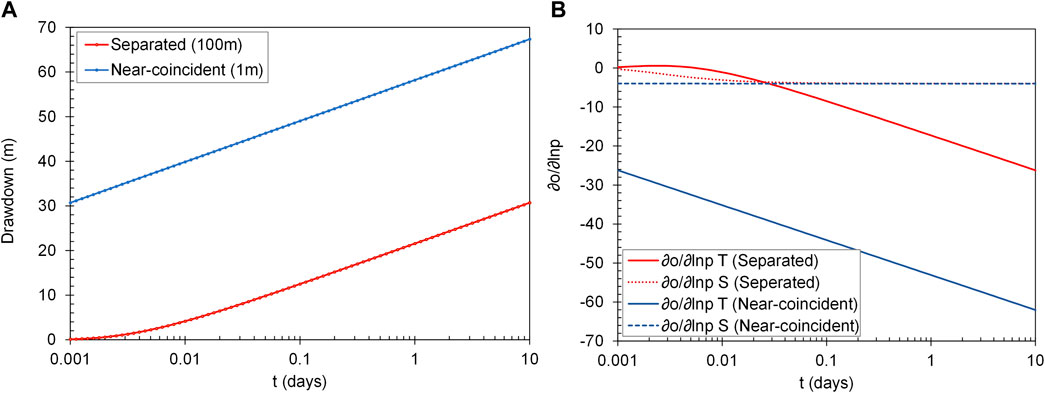
FIGURE 2. (A) Drawdown in the observation well. (B) The derivative of drawdown with respect to the natural logs of global T and S.

3.2 Spatially integrated kernels

At any time during an aquifer test, the submatrices appearing in Eqs 21 and 23 can be computed in the manner described above. As such, they pertain to aquifer test interpretation that is based on drawdowns that are sampled up until that time. Each row of these submatrices comprises an integration kernel. In accordance with Eq. 19 each element in each row is multiplied by the corresponding element of k; that is, it is multiplied by T, T_x, T_y or S pertaining to a point within the aquifer. These values are then summed as a proxy for spatial integration.

Numerical integration of these kernels on their own yields the following results at all times.

$\underset{A}{{\displaystyle \int }}{R}_{\underset{¯}{T}-T}^{\prime }\left(\mathit{x}\right)d\mathit{x}=1.0(\mathrm{24a})$

$\underset{A}{{\displaystyle \int }}{R}_{\underset{¯}{T}-T_x}^{\prime }\left(\mathit{x}\right)d\mathit{x}=0.5(\mathrm{24b})$

$\underset{A}{{\displaystyle \int }}{R}_{\underset{¯}{T}-T_y}^{\prime }\left(\mathit{x}\right)d\mathit{x}=0.5(\mathrm{24c})$

$\underset{A}{{\displaystyle \int }}{R}_{\underset{¯}{T}-S}^{\prime }\left(\mathit{x}\right)d\mathit{x}=0.0(\mathrm{24d})$

$\underset{A}{{\displaystyle \int }}{R}_{\underset{¯}{S}-T}^{\prime }\left(\mathit{x}\right)d\mathit{x}=0.0(24e)$

$\underset{A}{{\displaystyle \int }}{R}_{\underset{¯}{S}-T_x}^{\prime }\left(\mathit{x}\right)d\mathit{x}=-0.5(\mathrm{24f})$

$\underset{A}{{\displaystyle \int }}{R}_{\underset{¯}{S}-T_y}^{\prime }\left(\mathit{x}\right)d\mathit{x}=0.5(\mathrm{24g})$

$\underset{A}{{\displaystyle \int }}{R}_{\underset{¯}{S}-S}^{\prime }\left(\mathit{x}\right)d\mathit{x}=1.0(\mathrm{24h})$

Collectively, Eqs 24a, 24d, 24e, 24h imply that the inverse problem is well-posed, for if the aquifer is homogeneous, values of T and S calculated using Eq. 18 are estimates of the true, global values of T and S.

Equations 24b, 24c, 24f, 24g are noteworthy. Suppose that T_x is multiplied by a factor c and that T_y is divided by this same factor. (Note that multiplication becomes addition in the log domain). This introduces horizontal anisotropy to the aquifer. According to the above equations, the estimated T is unchanged; it is therefore equal to the geometric mean of T_x and T_y. In contrast, estimated S is altered because the right sides of Eqs 24f and 24g have opposite signs; its value is decreased by a factor of c. However, if the real value of S throughout the aquifer is then multiplied by c, estimated S returns to its original value. Use of a variant of the Theis equation that accommodates aquifer anisotropy (Papadopulos, 1965) verifies that drawdowns at the observation well are unchanged under these conditions.

The integrals that are presented in Eqs 24a to 24h can assist in interpreting the kernel maps that are discussed below. For example, early-time values of R′_T−T for the separated-well case are significantly negative in some areas. These must be balanced by areas of R′_T−T positivity so that the negative contribution to the total integral is not only cancelled, but integrates to 1.0. These positive values may be spread out over large areas, and so may not be as obvious as intensely negative values when plotted in space. Similarly, areas of negative R′_S–T must be balanced by areas of positive R′_S−T so that R′_S−T spatially integrates to zero.

3.3 Maps of spatial averaging function for separated wells

This section provides maps of R′_X−Y where X is either T or S and Y is either T, T_x, T_y or S. Maps are presented for five different times. In each case, the map pertains to Theis-based interpretation of observation well drawdowns acquired up until that time. In all of these figures, red is indicative of positive values while blue indicates negative values. Shading is linear; the zero contour is highlighted. When viewing these plots, keep in mind that it is their spatial integral that matters, for this is what determines an estimated value of T or S.

The Supplementary Material presents these same maps, but with logarithmic shading. This reveals the spatial characteristics of these functions in low-intensity areas that are distant from the pumping and observation wells. Because these areas are large, they make significant contributions to the spatial integrals though which T and S are calculated.

R′_T−T is mapped in Figure 3. Unsurprisingly, contributions of real T to estimated T expand outward from the pumping and observation wells with time, diminishing in magnitude, but covering a broader area. At larger times, contours of equal R′_T−T form ellipses with foci at the pumping and observation wells. In contrast, the early-time pattern is complex, with high values between the wells, and within lobes that extend beyond the wells. Small negative cusps lie to the north and south of the line that joins the wells. These negative cusps diminish in intensity with increasing time, but never completely disappear.

FIGURE 3

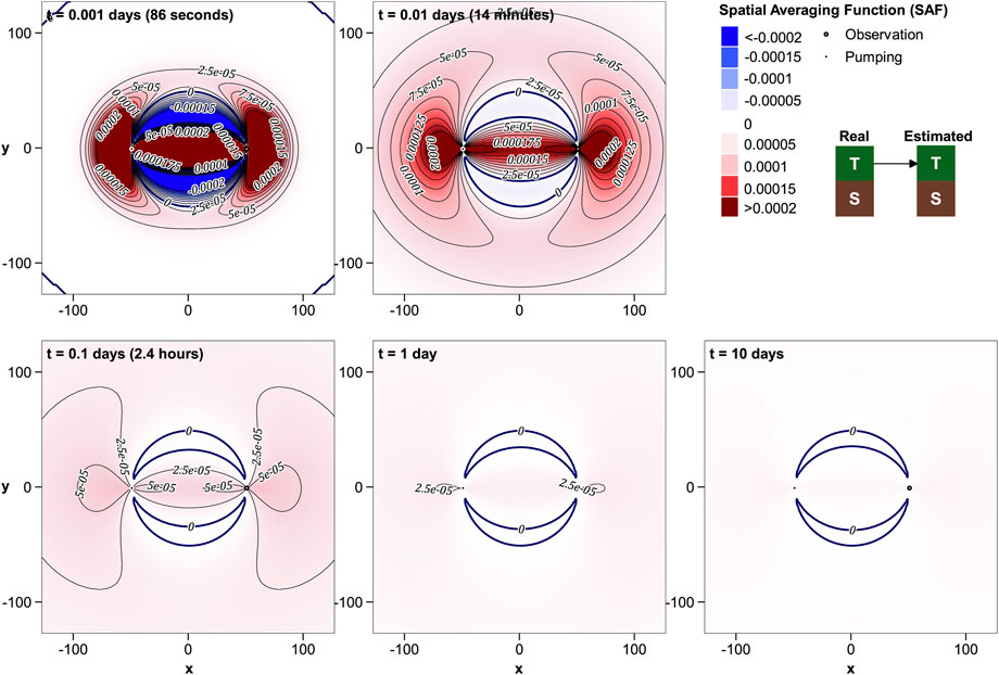
FIGURE 3. R′_T−T for separated wells at five different times.

Figures 4, 5 show that contributions made by real-world T_x and T_y to Theis-estimated T are more complex than that made by T alone. (See also the plots in the Supplementary Material where logarithmic shading is employed.) Local T anisotropy close to and between the wells can strongly affect estimated T at very early times. However, contributions from these areas fade with time as smoother R'_T−Tx and R′_T−Ty kernels expand beyond the wells. At large times, estimated T reflects true T_x that prevails at large distances along the x axis and true T_y that prevails at large distances along the y axis. Reciprocally, T_y at large distances along the x axis and T_x at large distances along the y axis have little effect on estimated T. That is to say, estimated T reflects components of directional real-world T that point towards the wells.

FIGURE 4

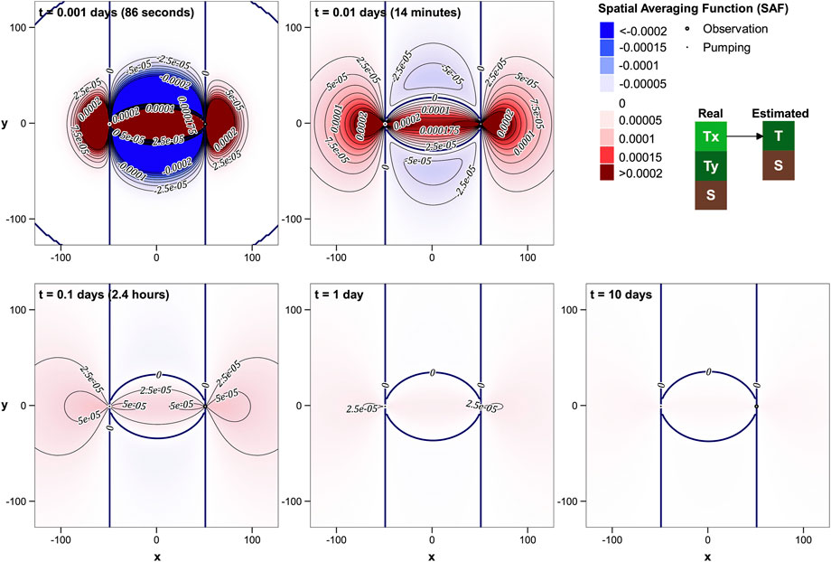
FIGURE 4. R′_T−Tx for separated wells at five different times.

FIGURE 5

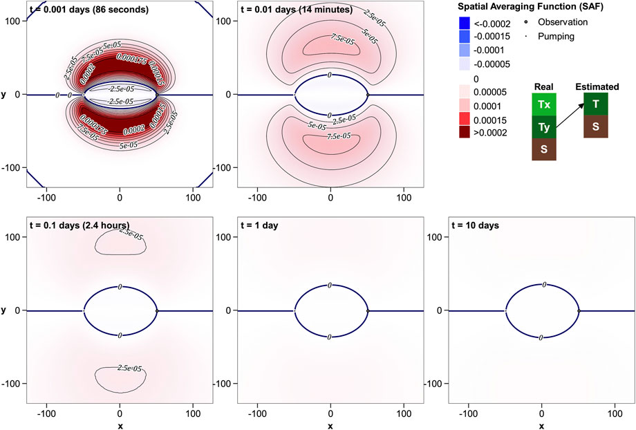
FIGURE 5. R′_T−Ty for separated wells at five different times.

Figure 6 depicts the potential for contamination of estimated T by real-world S. At early times, real-world S between the extraction and observation wells can exert a considerable influence on estimated T. Positive and negative contributions of S to T are strong, but collectively integrate to zero as outlined above.

FIGURE 6

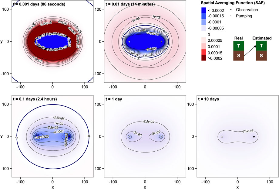
FIGURE 6. R′_T−S for separated wells at five different times.

The presence of a significant band of negatively-valued R′_T-S joining the pumping well to the observation well at early times is easily explained. Low storativity in this area hastens propagation of drawdown to the observation well; it therefore “looks like” high local T. This affects estimated T shortly after the commencement of pumping when the derivative of drawdown with respect to global S and global T are both positive; see Figure 2B. At later times, contributions of real-world S to estimated T become more diffuse. However an area of anomalous S between the pumping and observation wells is never quite “forgotten” by the Theis-based parameter estimation process.

Figure 7 maps the contribution to estimated S by real-world S. In contrast to spatial averaging functions that affect estimated T, areas that contribute to estimated S tend to remain close to the pumping and observation wells even at late times. At very early times the pattern is complex; the wells are joined by a sliver of intensely negative S contribution to S; this is surrounded by areas of intensely positive contributions of S to S.

FIGURE 7

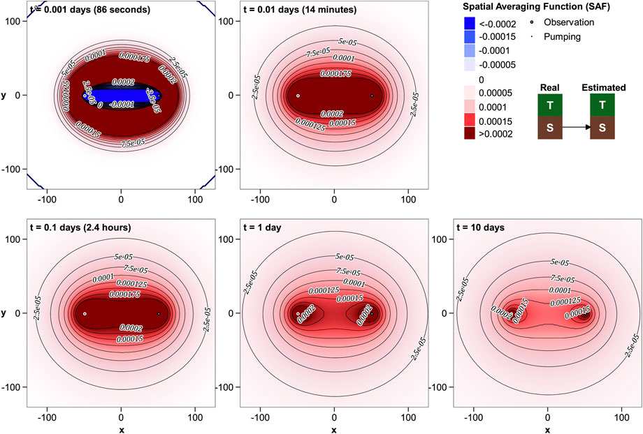
FIGURE 7. R′_S−S for separated wells at five different times.

The limited expansion of R′_S−S with time (and of other R′_S-X maps shown below) implies that estimates of S forthcoming from aquifer test analysis pertain to a smaller area than do estimates of T. Furthermore, this disparity in area grows with the length of the test. These maps also imply that information pertaining to aquifer storativity ceases to be acquired after a relatively short time during a pumping test. This accords with identification by authors such as Kruseman and de Ridder (1990) of a pseudo-steady-state phase of drawdown development as time proceeds.

Figures 8–10 suggest a high potential for contamination of estimated S by between-well T, especially T_x. High values of T_x in this area can hasten propagation of drawdown from the pumping well to the observation well, thereby replicating the impact of low S. This effect is strong, and does not dissipate with time. In hydrogeological contexts where the natural variability of T is much greater than that of S, the potential for contamination of estimated S by between-well anomalies in T may be very high.

FIGURE 8

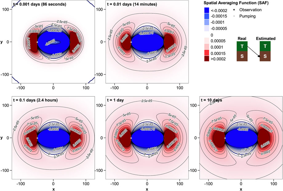
FIGURE 8. R′_S−T for separated wells at five different times.

FIGURE 9

FIGURE 9. R′_S−Tx for separated wells at five different times.

FIGURE 10

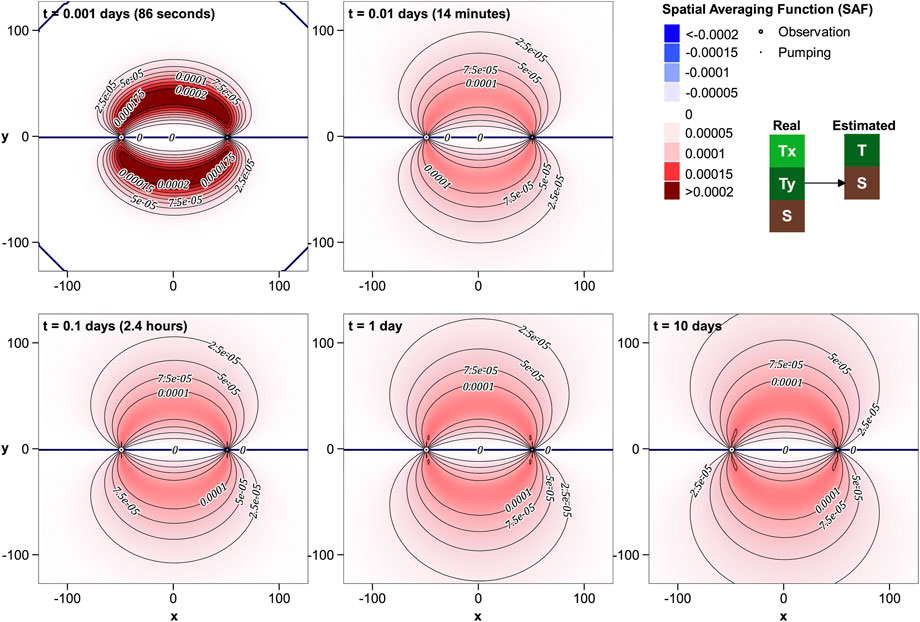
FIGURE 10. R′_S−Ty for separated wells at five different times.

The impact of real-world T_y on estimated S is complex. Like that of T, it persists to late times. The near-well cusps of positive influence suggest that strategically-located areas of high T_y can gather water from distant areas that can slow the growth of drawdown in the observation well. This appears as high global S where these drawdowns are subjected to Theis interpretation.

3.4 Maps of spatial averaging function for near-coincident wells

As stated above, calculations for coincident wells are complicated by non-integrable singularities in Fréchet kernels. To avoid this problem, wells are placed 1 m apart. Furthermore, we do not provide maps of R'_S-X for the near-coincident case because S cannot be estimated unless a dedicated observation well is employed.

From Figures 11–14 it is apparent that maps of R′_T−T and R′_T−S are radially symmetric, while those of R′_T−Tx and R′_T−Ty are not. This is because anisotropy is the only thing that distinguishes one direction from another when the pumping and observation wells are coincident.

FIGURE 11

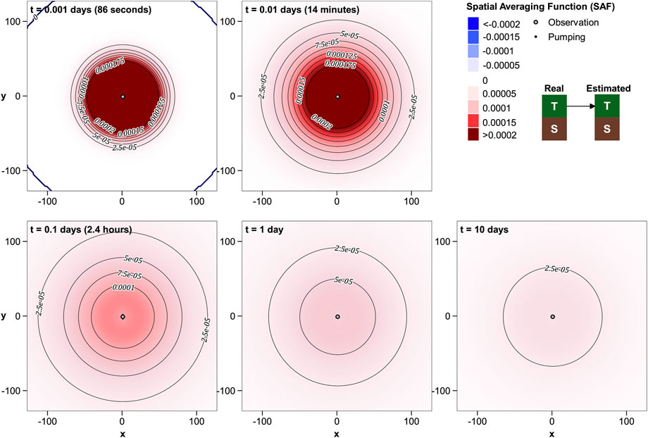
FIGURE 11. R′_T−T for near-coincident wells at five different times.

FIGURE 12

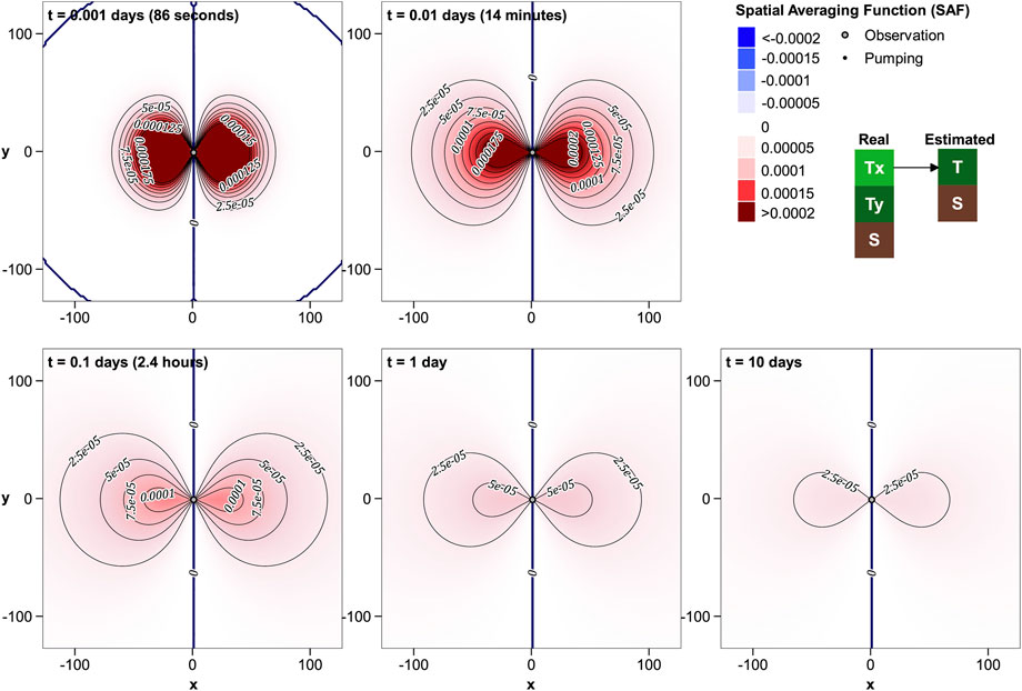
FIGURE 12. R′_T−Tx for near-coincident wells at five different times.

FIGURE 13

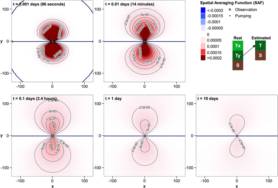
FIGURE 13. R′_T−Ty for near-coincident wells at five different times.

FIGURE 14

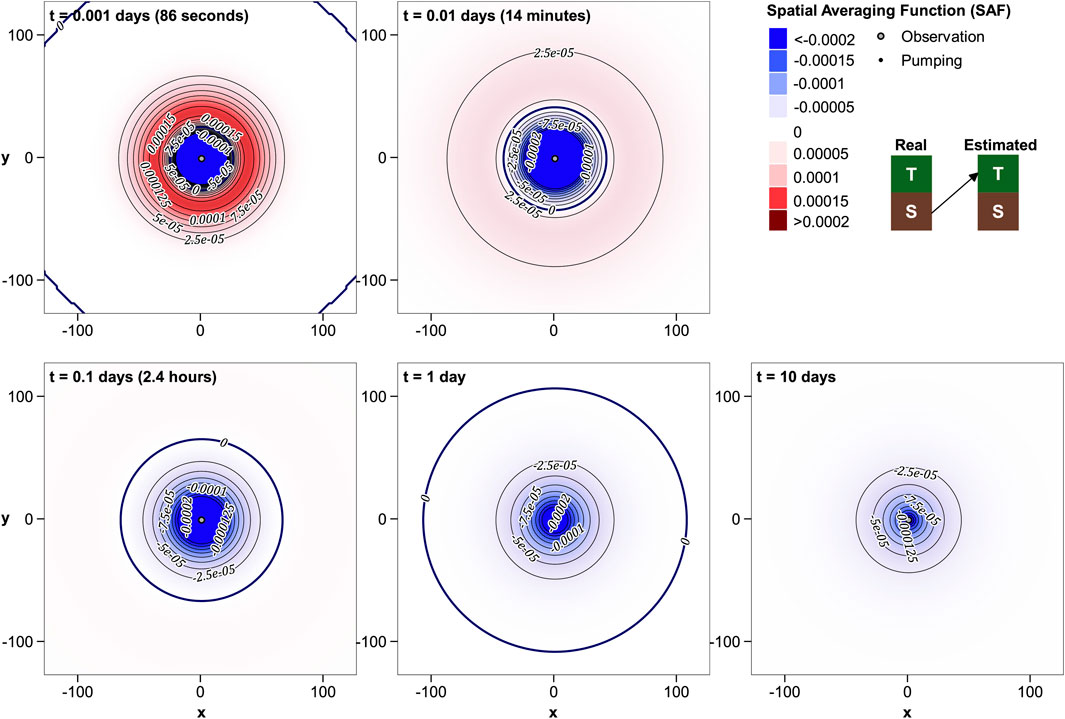
FIGURE 14. R′_T−S for near-coincident wells at five different times.

Figure 11 demonstrates that R′_T−T expands continuously with time, and is ubiquitously positive. Its rate of expansion is not quite as fast as for separated wells. R′_T−Tx and R′_T−Ty also maintain positivity over time and space. Their lobate shapes indicate that estimated T is influenced by T_y that prevails in the positive and negative y directions from the pumping well and by T_x that prevails in the positive and negative x directions from this well. These are the directions from which water flows towards the pumped well. Because x and y directions are arbitrary for coincident wells, a more general (but unsurprising) conclusion follows. It is that estimated T reflects the component of real-world T that points in the direction of the pumped well.

Figure 14 shows that near-well, real-world S can have a strong negative influence on estimated T at early times. Its influence is somewhat subdued at later times, but is never completely forgotten.

3.5 Radius of investigation

The radius of investigation of an aquifer test is discussed by a number of the authors that are cited in the introduction to this paper; see Bresciani et al. (2020) for a review. Different definitions highlight different aspects of drawdown propagation, and of responsiveness of drawdown to the presence of a distant barrier. The subject matter of the present paper suggests an additional definition, this being based on the area of aquifer that contributes to Theis-estimated T.

As stated above, for separated wells contours of R′_T−T at large distances from the pumping and observation wells form ellipses with foci at these wells. These ellipses collapse to circles for coincident wells. We (somewhat arbitrarily) define the radius of investigation of an aquifer test as the length of the major semi-axis of an ellipse that encloses an area that contributes all but 10% to the estimated value of T. Thus R′_T−T within the ellipse integrates to 0.9. (Note that the lengths of the semi-major and semi-minor axes of this ellipse are almost equal at large distances from the wells).

In Figure 15 the radius of investigation is plotted against time for both separated and near-coincident wells. It is apparent from this figure that T inferred from drawdowns that are measured in a separate observation well “feels” more of the surrounding real-world T than T that is inferred from drawdowns in a pumping well. Supposedly, this increased area of spatial averaging provides greater immunity from the effects of near-well anomalies in real-world S and T. However it renders estimated T more susceptible to the effects of system boundaries. It is of interest to note that the difference in radius of influence between the separated and near-coincident cases grows with time. For the parameters we chose for this example it is roughly equal to the well separation after 0.5 days, and grows to more than double this after 10 days.

FIGURE 15

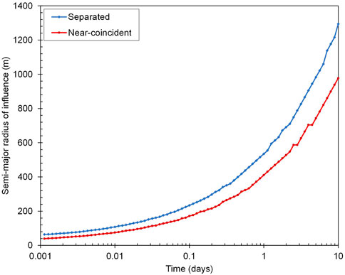
FIGURE 15. Radius of semi-major axis of ellipse of influence for separated and near-coincident wells.

4 Discussion

Work that is documented herein extends previous investigations into the relationship between aquifer-test-inferred hydraulic properties and real-world hydraulic properties. We have formulated spatial averaging functions that map real-world T, T_x, T_y and S to estimated T and S under the assumption that the latter are estimated by fitting a Theis curve to drawdown measurements. The analysis can be readily extended to accommodate the fitting of other types of curves to raw or processed drawdowns. These averaging functions are approximate, for their formulation assumes only small departures from hydraulic property uniformity. Nevertheless, the insights that they provide are highly instructive.

Values of T and S that emerge from interpretation of aquifer test data can be viewed as complex spatial averages of real-world T and S over an area that expands with time. These averaging functions cross parameter boundaries. Hence local anomalies in real-world T can influence the estimated value of S and vice versa.

The area over which real-world hydraulic properties are averaged to estimate T is greater than that over which they are averaged to estimate S. The difference between these two areas grows with pumping time. Hence aquifer-test-estimated S tends to reflect real-world S in closer proximity to the pumping and observation wells than estimates of T reflect real-world T. At the same time, estimates of S are vulnerable to corruption by near-well anomalies in T. The reverse applies for pumping tests of short duration; that is, estimates of T can be corrupted by near-well anomalies in S. Importantly however, as the time over which drawdown data are acquired increases and the area over which T is averaged expands, opportunities for contamination of estimated T by S decrease. During this period the relationship between drawdown and the log of time approaches linearity, and direct estimates of T are available through Cooper-Jacob (1946) analysis of the slope of the drawdown line. It follows that estimates of S forthcoming from aquifer test analysis are often less reliable than those of T, and may be somewhat dependent on the disposition of T between the pumping and observation wells. This is not a new conclusion; see, for example, Sanchez-Vila et al. (1999) and Trinchero et al. (2008).

Intuition may suggest that separation of pumping and observation wells yields insights into between-well T. Analyses that are presented herein show that this applies for only a very short time. Thereafter, significant contributions to interpreted T are made by material that is beyond both of the extraction and measurement wells. The longer an aquifer test proceeds, the less does the separation of the wells, or the material between them matter, and the more does the zone of expanding contribution of real T to inferred T expand into an area that surrounds both of these wells.

At no time during an aquifer test does estimated T reflect real-world T_x more than real-world T_y regardless of the offset direction of the observation well with respect to the pumping well. However, the manner in which distributed T_x and T_y are spatially averaged is very different. At very early times, estimated T is positively influenced by T_x along the line that joins the wells. However, it is also negatively influenced by both T_x and T_y to the north and south of this line. As time goes on, estimated T is much more reflective of the component of real-world T that points towards the midpoint of the wells than it is of the component of T in any other direction.

Once a certain amount of time has elapsed, the radius of investigation of a separated-well aquifer test becomes greater than that of a coincident-well aquifer test. The ratio of the two investigation radii continues to grow thereafter. The greater averaging area for separated wells protects estimated T from contamination by anomalies in near-well T and S. However, it renders it more vulnerable to the effects of hydrogeological boundaries.

We close the discussion by noting that this paper does not address uncertainties of estimated T and S. It would not be a difficult matter to derive expressions for these uncertainties using the theory presented above. However this would require statistical characterisation of the spatial heterogeneity of subsurface T and S, including the scale of this heterogeneity. This is beyond the scope of the present paper. Furthermore, it can be argued that characterisation of the uncertainties of the complex spatial averages of T and S that are depicted herein may be of limited use to managers of a groundwater system. Of greater use are the uncertainties of arithmetic or geometric averages of system properties over user-specified areas, for example, circles or ellipses that circumscribe the pumping test wells, or the cells of a groundwater model grid that spans the area affected by pumping-induced drawdowns. These too can be calculated through a simple extension of the theory provided herein; this will be addressed in future work.

5 Conclusion

The relationships between aquifer-test-inferred transmissivity and storativity and those that prevail in a heterogeneous real world are complex, and sometimes non-intuitive, particularly at early pumping times.

Insights into these relationships provided by the present study can inform the design of an aquifer test. A matter of particular interest at some sites may be whether observation wells should be specially drilled so that pumping-induced drawdowns can be measured at one or a number of distances and directions from the pumped well. The incentive for such a design may be the gathering of information on near-well hydraulic property heterogeneity.

Results presented herein suggest that if insights into near-well hydraulic property heterogeneity are sought, then there is no need to pump for a long time, for this information emerges early in an aquifer test. They also suggest that considerable sophistication is required in interpreting multi-well drawdown data if this information is to be retrieved. This sophistication extends well beyond Theis-based analysis of drawdown in individual wells; the complex averaging functions that link real-world hydraulic properties to Theis-estimated T and S hide more than they reveal.

An issue of considerable importance is how estimates of transmissivity made through historical interpretation of aquifer test data should be used in parameterisation of a groundwater model. Before construction of a groundwater model, the outcomes of previous hydrogeological investigations that have been undertaken within its domain are generally reviewed. They often reveal that many aquifer tests have been conducted in the study area, some involving a single well, and some involving one or multiple observation wells. In most cases, drawdowns have been interpreted using Theis of Jacob-Cooper analysis.

The present study suggests that estimates of local transmissivity and storativity (particularly the latter) obtained in this way should be treated with caution. The spatial averaging of local hydraulic properties that is implied in these estimates may preclude their direct transferral to proximal cells of a groundwater model. At the same time, these estimates should not be ignored. An advantage of using linear analysis to establish the relationship between estimated and real-world hydraulic properties, is that an extension of this analysis can provide estimates of error variance between hydraulic properties averaged over model cells and those obtained through aquifer test interpretation. Probabilistic parameterisation of proximal groundwater model cells can then follow. This is the subject of an ensuing paper.

Data availability statement

The raw data supporting the conclusion of this article will be made available by the authors, without undue reservation.

Author contributions

NM designed the analytical models, wrote software to generate the Frechet kernels/spatial averaging function and interpreted the results. He created all figures and wrote the majority of the paper. JD provided guidance on the concepts, linear algebra and Fortran functions to calculate the spatial averaging function. He assisted with interpreting the results and writing the paper. PH provided guidance on the analytical model, helped interpret the results, and assisted writing/reviewing the paper.

Funding

This study was financially supported by the Groundwater Modelling Decision-Support Initiative (GMDSI—https://gmdsi.org/).

Conflict of interest

Author JD was employed by Watermark Numerical Computing.

The remaining authors declare that the research was conducted in the absence of any commercial or financial relationships that could be construed as a potential conflict of interest.

Publisher’s note

All claims expressed in this article are solely those of the authors and do not necessarily represent those of their affiliated organizations, or those of the publisher, the editors and the reviewers. Any product that may be evaluated in this article, or claim that may be made by its manufacturer, is not guaranteed or endorsed by the publisher.

Supplementary material

The Supplementary Material for this article can be found online at: https://www.frontiersin.org/articles/10.3389/feart.2022.1079287/full#supplementary-material

References

Aster, R. C., Borchers, B., and Thurber, C. H. (2019). Parameter estimation and inverse problems. 3rd. Amsterdam, Netherland: Springer.

Google Scholar

Bresciani, E., Shandilya, R. N., Kang, P. K., and Lee, S. (2020). Well radius of influence and radius of investigation: What exactly are they and how to estimate them? J. Hydrology 583, 124646. doi:10.1016/j.jhydrol.2020.124646

CrossRef Full Text | Google Scholar

Butler, J. J. (1988). Pumping tests in nonuniform aquifers - the radially symmetric case. J. Hydrology 101, 15–30. doi:10.1016/0022-1694(88)90025-x

CrossRef Full Text | Google Scholar

Butler, J. J. (1990). The role of pumping tests in site characterization: Some theoretical considerations. Ground Water 28 (3), 394–402. doi:10.1111/j.1745-6584.1990.tb02269.x

CrossRef Full Text | Google Scholar

Cooley, R., and Christensen, S. (2006). Bias and uncertainty in regression-calibrated models of groundwater flow in heterogeneous media. Adv. Water Resour. 29, 639–656. doi:10.1016/j.advwatres.2005.07.012

CrossRef Full Text | Google Scholar

Cooley, R. L. (2004). A theory for modeling ground-water flow in heterogenous media. US Geological Survey Professional Paper, Washington, DC, USA, 1679, 220.

Google Scholar

Cooper, H. H., and Jacob, C. E. (1946). A generalized graphical method for evaluating formation constants and summarizing well-field history. Am. Geophys. Union 27 (4), 526–534. doi:10.1029/tr027i004p00526

CrossRef Full Text | Google Scholar

Copty, N. K., Trinchero, P., and Sanchez-Vila, X. (2011). Inferring spatial distribution of the radially integrated transmissivity from pumping tests in heterogeneous confined aquifers: Analysis of pumping tests in confined aquifers. Water Resour. Res. 47 (5). doi:10.1029/2010wr009877

CrossRef Full Text | Google Scholar

Doherty, J. (2015). Calibration and uncertainty analysis for complex environmental models. Brisbane, Australia: Watermark Numerical Computing.

Google Scholar

Draper, N. R., and Smith, H. (1998). Applied regression analysis. 3rd. Wiley-Interscience, Hoboken, NJ, USA.

Google Scholar

Knight, J. H., and Kluitenberg, G. J. (2005). Some analytical solutions for sensitivity of well tests to variations in storativity and transmissivity. Adv. Water Resour. 28 (10), 1057–1075. doi:10.1016/j.advwatres.2004.08.018

CrossRef Full Text | Google Scholar

Kruseman, G. P., and de Ridder, N. A. (1990). Analysis and evaluation of pumping test data. 2nd. Wageningen, Netherland: International Institute for Land Reclamation and Improvement.

Google Scholar

Leven, C., and Dietrich, P. (2006). What information can we get from pumping tests?-comparing pumping test configurations using sensitivity coefficients. J. Hydrology 319 (1-4), 199–215. doi:10.1016/j.jhydrol.2005.06.030

CrossRef Full Text | Google Scholar

Menke, W. (2018). “Geophysical data analysis,” in Discrete inverse theory. 4th (Academic Press) Cambridge, MA, USA.

Google Scholar

Moore, C., and Doherty, J. (2006). The cost of uniqueness in groundwater model calibration. Adv. Water Resour. 29 (4), 605–623. doi:10.1016/j.advwatres.2005.07.003

CrossRef Full Text | Google Scholar

Oliver, D. S. (1990). The averaging process in permeability estimation from well-test data. SPE Form. Eval. 5 (3), 319–324. doi:10.2118/19845-pa

CrossRef Full Text | Google Scholar

Oliver, D. S. (1993). The influence of nonuniform transmissivity and storativity on drawdown. Water Resour. Res. 29 (1), 169–178. doi:10.1029/92wr02061

CrossRef Full Text | Google Scholar

Papadopulos, I. S. (1965). Nonsteady flow to a well in an infinite anisotropic aquifer: Proceedings of the dubrovnik symposium on the hydrology of fractured rocks. Wallingford, UK: International Association of Scientific Hydrology.

Google Scholar

Sánchez-Vila, X., Meier, P. M., and Carrera, J. (1999). Pumping tests in heterogeneous aquifers: An analytical study of what can be obtained from their interpretation using Jacob's Method. Water Resour. Res. 35 (4), 943–952. doi:10.1029/1999wr900007

CrossRef Full Text | Google Scholar

Theis, C. V. (1935). The relation between the lowering of the piezometric surface and the rate and duration of discharge of a well using groundwater storage. Am. Geophys. Union Trans. 16, 519–524. doi:10.1029/tr016i002p00519

CrossRef Full Text | Google Scholar

Trinchero, P., Sanchez-Vila, X., and Fernandez-Garcia, D. (2008). Point-to-point connectivity, an abstract concept or a key issue for risk assessment studies? Adv. Water Resour. 31, 1742–1753. doi:10.1016/j.advwatres.2008.09.001

CrossRef Full Text | Google Scholar

Zha, Y., Shi, L., Liang, Y., Michael Tso, C.-H., Zeng, W., and Zhang, Y. (2020). Analytical sensitivity map of head observations on heterogeneous hydraulic parameters via the sensitivity equation method. J. Hydrology 591, 125282. doi:10.1016/j.jhydrol.2020.125282

CrossRef Full Text | Google Scholar