A subterranean estuarine typology analogous to open-water estuaries

1 Introduction

Subterranean estuaries (STEs) are recognized as “important interconnected systems driving water quality, ecology and biogeochemical cycles in nearby coastal ecosystem” (Rocha et al., 2021). Although they are ubiquitous along the world’s shore, their manifestations, and hence, their impacts, are as diverse as coastlines themselves. Being unseen and laying along the boundaries of traditional, disciplinary investigators, they can be difficult to study. Although expansive study is necessary in order to incorporate these important features, site specific studies can be far and few between. A typology for STEs may be useful in identifying data gaps and interpolating or extrapolating available information. There should be a typology, so this article considers elements of such a typology in the context of open-water estuaries.

2 Classification as a typology

Typology is the study, analysis or classification based on type. Our necessarily imperfect understanding of the complex interactions that characterize STEs and restriction of both human and financial resources available to carry out required studies are all limitations which plaque investigators. The typological approach is an attempt to circumvent obstacles caused by a paucity of direct measurements, a lack of offshore and subsurface data, and data gaps. A typology for STEs is intended to focus attention on the most important areas and to help extrapolate existing data.

A topology for STEs is not a model, but rather recognition that a few parameters that are pervasive in the manifestation of STEs. A complete list of parameters, as needed to generate a dynamic model of an STE, would be extensive and certainly not all would be widely known. Some, however, might be catalogued globally and it is to be hoped that a small set of these might provide typological discrimination. A typology would look for a set of relevant parameters, but proxy parameters and indirect indicators also might be employed as surrogates to assess the impacts of poorly resolved processes (Bokuniewicz 2001). As an example, I had attempted to construct a typology for submarine groundwater discharge (SGD) by dividing the world’s coast into sections based on four parameters. These were 1) areas of high “steepness”, 2) areas of high runoff and medium “steepness”, 3) areas of medium evapotranspiration, low runoff and low “steepness”, 4) areas of high evapotranspiration low runoff and low steepness; 5) areas of medium “steepness” low evapotranspiration and low runoff, and 6) low evapotranspiration, low “steepness” and low runoff (Bokuniewicz et al., 2003).

By analogy with open-water estuaries, I suggest here that the salinity structure might be used typologically. In the STE, the density-driven flow of seawater landward is equivalent to the estuarine circulation. More saline groundwater flows landward into the coastal aquifer driven by hydraulic dispersion (e.g., Kohout 1960). At the same time, fresher groundwater flows seaward above it driven by terrestrial hydraulic gradients. Although much less intense than the mixing and dispersion caused by waves and tides in open water, the dispersion of salt in brackish groundwater in STEs must be large enough to produce gravitational movement of brackish water landward and upward in response to the hydraulic gradient, giving STEs a definable structure.

The STE, however, has another characteristic rarely shared with open-water estuaries. On the intertidal surface of an STE, the flooding sea water percolates down to form an upper salinity zone of saline water by gravitational convection and the density inversion subtidally drives saltwater into underlying fresher groundwater. This gives the STE an upper salinity plume (USP) usually expected in the intertidal zone but potentially extending subtidally, perhaps by salt-fingering (e.g., Boufadel 2000; Robinson et al., 2006). The top of the STE, that is the intertidal or subtidal sea floor, therefore, exhibits an inverted salinity gradient¹.

3 Parameters estuarine classification

The earliest definitions of an estuary (Lyell 1834 or, perhaps, Varro c. 45 BCE²) referred simply to embayments entered by both a river and the tides of the sea. Basic criteria for the existence of estuaries, open-water or otherwise, include two fundamental elements: a) the presence of a watershed freshwater source and b) a free connection to the adjacent sea. Together, they allow the combination of the two water masses into a mixture that is chemically distinct from the original solutions. The two main physical drivers of mixing within the intermediate space are the tidal forcing and the seawater-freshwater flow potential, which, in the case STEs. Is regulated by the hydraulic gradient on land and the hydraulic conductivity of the aquifer (Robinson et al., 2006). All estuarine waters are products of mixing and all estuaries identifiable as mixing zones. These two phenomena, the river, and the tides, provide the rationale for defining open-water estuaries based on their salinity structure. The mixing between saltwater and freshwater was later appropriately recognized as the fundamental discriminator among open water estuaries (Ketchum 1951; McHugh, 1967).

The Venice system (Anonymous 1959) established five estuarine zones based on salinity. These were 1) limnetic, exhibiting salinities less than <0.5; 2) oligohaline, with salinities between 0.5 and 5; 3) mesohaline, with salinities from 5 to 18; 4) polyhaline, having salinities from 18 to 30 and 5) eurylhaline, where salinity is greater than 30. This widely used classification represented biologically relevant niches. In fact, the presence of eurylhaline species was sometimes used in the definition of an open-water estuary as an indication of the stability and persistence of mixed conditions (Perillo 1995). The system was revisited and revised into five overlapping zones based on observed ecosystems (Bulger et al., 1993); these were characterized by salinities of 4, of between 2 and 14; from 11 to 18; from 16 to 27; and salinity greater than 24.

Although some definitions of open-water estuaries include the presence of eurylhaline species, the biological manifestations in STEs are probably too limited to be used in a typology. In STEs, the ecological aspects are primarily confined to the impacts of submarine groundwater discharge (SGD) at the sea floor above the STE. SGD reduces the pore-water salinity and supplies nutrients. These vectors affect distribution and zonation of nearshore benthic communities, as well as productivity and biomass in the coastal ocean (e.g.,Valiela et al., 1990; Knee and Paytan 2011). SGD also may change the substrate grain-size and the morphology of the seafloor, as well as redox and pH conditions. The effects of SGD on biological communities have been proposed and documented both on macrofauna communities (e.g., Miller and Ullman 2004; Silva et al., 2012) as well as meiofaunal assemblages (Kotwicki et al., 2014; Grezlac et al., 2018). A typological discriminator could be the gradient of eurylhaline benthic species at the shoreline, however such data are rare to non-existent, and as pointed out by an astute reviewer, microbiology communities may have the potential to characterize certain salinity ranges in STEs but have not been adequately studied in detail. So, we must forgo their use in a typology at this stage.

Besides any biological relevance, the salinity structure provided by the mixing of seawater and saltwater forms a basic classification of estuaries as well-mixed, stratified or partially mixed based on the salinity stratification. Where tidal mixing is small compared to river input, salt-wedge (SW) and well-stratified estuaries exhibit a sharp pycnocline separating the upper layer of fresher water and the bottom layer of more saline water. SW estuaries are fairly rare because they require a high fluvial discharge to retard salt water from entering through the surface, and a great depth to inhibit mixing. The Mississippi River is a good example of a SW estuary. As the ratio of tidal flow to river flow increases, turbulent mixing forms, first, a partially stratified water column widening the pycnocline, and then, a well-mixed estuary. All forms require the flow of denser, more saline, waters landward into the estuary, almost always at the sea floor, while fresher (surface) waters flow seaward. The dispersion of salt must be large enough to produce gravitational movement of brackish water landward and upward in response to the hydraulic gradient (Perillo 1995). Employing these principles, one classification of open-water estuaries has been based on the salinity stratification and a circulation parameter expressed as the ratio of the net open-water surface current to the mean freshwater flow (Hansen and Rattray 1966).

The distribution of salinity zones and consequent circulation can be the defining features of STEs as well. The seepage of fresh groundwater into the STE is equivalent to the river flow into the open-water estuary and the landward migration of sea salt in the saline groundwater. Its upward advection in STEs is driven by changes in density due to mixing along the flow path. This dispersion-driven recirculation generates the SW in the lower sections of the STE (e.g., Boufadel 2000; Robinson et al., 2006). By this analogy with open-water estuaries, I suggest here that the salinity structure might be used typologically.

Open-water estuaries are classified also by their morphology. Open-water estuaries are recognized as distinct bodies of water, described as “semi-enclosed” in many definitions (e.g., Pritchard 1960; Perillo 1995). The geomorphic classification of estuaries relies on mapping their lateral boundaries (their shorelines) and the nature of their connection to the sea (their inlets or mouths). Some STEs can also be delineated in this way, but not all or even most. Those that can include valley-filled aquifers of alluvial, saprolite, or glacial unconsolidated sediment extending under the sea. More commonly, however, STEs exist on open coasts with lateral and seaward boundaries invisible and ill-defined. STEs might be considered just another type of estuary as defined for open-water estuaries, except the limits of the low Reynolds number approximation of the Navier-Stokes equation³ which requires the dominant control of permeability. In terms of STEs, such a morphological classification may be analogous to classes where the hydraulic conductivity rather than the physical shape of the basin is the discriminator. A classification of the coastal aquifers by the type of hydraulic conductivity, for example, would include five types as would be found in 1) sandstone, 2) interbedded sandstone and carbonate, 3) semi consolidated carbonate, 4) basalt and other types of volcanic and 5) an “other rock” category (http://nationalatlas.gov/aquifersm.html; accessed 2020). These could be subdivided further into types as a) water-table aquifers, b) confined aquifers or c) stacked aquifers like deltaic aquifers. In any event, the hydraulic conductivity control of salinity structure must be a basic foundation of a typology, but most readily applicable to unconsolidated aquifers as opposed to karstic or fractured rock.

4 Parameters of a typology for STEs

An attempt at a typology for STEs, therefore, might be based on parameters chosen to represent 1) the size of the USP, 2) the width of the outer zone of dispersion and 3) the length of the SW (Figure 1). Harkening back to Varro, the STE structure can be regarded as that part of the coastal aquifer where there is an influence on the salinity structure are the tides relevant to the hydraulics of mixing in the STE⁴. There are three impacts of the tide then relevant to the function of the STE. The first impact is merely the periodic flooding of the intertidal surface with sea water. The USP spans the intertidal zone which is the product of the beach slope (S) and the tidal range (H). Its thickness might be represented by the vertical distance the saltwater percolates downward over a tidal period (T). In the presence of an inverted salinity gradient, saline pore water penetration occurs at a rate of

$w=\Delta \rho /\rho \ast K/e(1)$

where w is the velocity of the leading edge, ρ is the fluid density, Δρ difference between the unmixed fluid end member, K is the hydraulic conductivity, and e the porosity (after Gosink and Baker 1990). Of course, the hydraulic conductivity, K, a controlling factor in parameterization of the salinity distribution (e.g., Glover 1964), is most easily handled in unconsolidated, isotropic, homogeneous aquifers. Classical models of the horizontal extend of the STE, for example, are approximated by a width of the outflow gap which is inversely proportional to K. A typologist might consider the vertical scale of the USP as the product of the K and the tidal period (T). The size of the USP scales, therefore, as

$\left(H*S\right)*\left(K*T\right)(2)$

with T often being the semidiurnal period of 12.42 h.

FIGURE 1

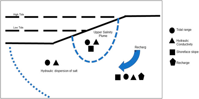
FIGURE 1. Basic structural parameters of the STE are represented by the proposed typological parameters.

Second, the rise and fall of the tide against a sloping shoreline propagates a tidally produced elevation in the hydraulic gradient into the coastal aquifer. This is commonly recognized as tidal pumping (Nielsen 1990). Tidal variation at the shoreline will propagate landward on the water table roughly at a speed dependent on the ratio of K and T (Metcalf 1995). The action of the tide against a sloping beach face elevates the mean hydraulic gradient landward of the shoreline and drives a component of the net seaward flow of groundwater landward of the shoreline due to the tidally induced over height. To a first approximation, the magnitude if this impact is calculated as (Nielsen 1990)

$0.5\left(H/S\right)\ast SQRT\left(e/2KTD\right)(3)$

That is, directly proportional to H, S and porosity (e) and inversely as K and thickness of the aquifer (D) and the tidal period (T). Although not to be treated here, it should be noted that waves would produce a comparable impact. For waves, the relevant parameter might be embodied in the Iribarren Number (Geng and Boufadel 2015), which, simply put, is the ratio of the beach slope to the square root of the wave steepness Wave steepness is the ratio of the wave height to the wavelength. The high frequency of incident waves compared to the tide may be treated as a dispersion around the still water level while changes in wave climate could produce variations in wave set-up on time scales comparable to the tide.

Third, the tidal action causes hydraulic dispersion throughout the aquifer which is essential to the recirculation of saline groundwater (Cooper 1964). It is this hydraulic dispersion that causes the change in density along the flow lines allowing seawater to gravitationally convect through the STE. The coefficient of hydraulic dispersion caused by the tide depends directly on K, H and T, as well as on the coefficient of storage, and inversely with the porosity and coefficient of transmissibility. The advance of the toe of the saltwater/freshwater interface inland as well as the width of the zone of dispersion seems to be universally related to the ratio of the hydraulic conductivity, K, divided by the freshwater recharge, Q_n (Doulgeris et al., 2020). At the same time, fresher groundwater flows seaward above the saltwater-freshwater interface are driven by the terrestrial hydraulic gradients. The reach of the terrestrial groundwater is the extent of SGD which is proportional to Q_n (Prieto and Destouni 2005). As a result, the flow of saline groundwater must reverse direction. Modeling showed that the landward flow of saline groundwater starts to reverse direction in the mesohaline zone and ends up flowing seaward in the limnetic zone (Oz et al., 2015).

The continuous introduction of marine groundwater by advection and hydraulic dispersion is fundamental to STEs. The width of the classical salt-water/freshwater interface, therefore, is a defining characteristic of the STE, and although influenced by several factors, the hydraulic dispersion due to the tide is a universal control. The freshwater recharge (Q_n) has been shown to be related to the width of the seaward zone of dispersion at the saltwater-freshwater interface and the extent of the STE, that is the reach of the saltwater intrusion at the base of the STE⁵. Considering these effects, in any event, the hydraulic dispersion, as well as the slope of the shore face, would have to be typological factors. With these considerations, I suggest that pervasive parameters (Table 1; Figure 1) are the hydraulic conductivity (K), the recharge (Q_n), the slope at the shoreline (S) and the tidal range (H assuming T of a semidiurnal tide). All the factors discussed have been explored globally (e.g., Gleeson et al., 2011; Mohan et al., 2018; Zamrsky et al., 2018; Athanasiou et al., 2019; Williams et al., 2019; Kirezci et al., 2020). Of these, hydraulic conductivity may be the most difficult to evaluate and might instead be replaced by aquifer type as a surrogate.

TABLE 1

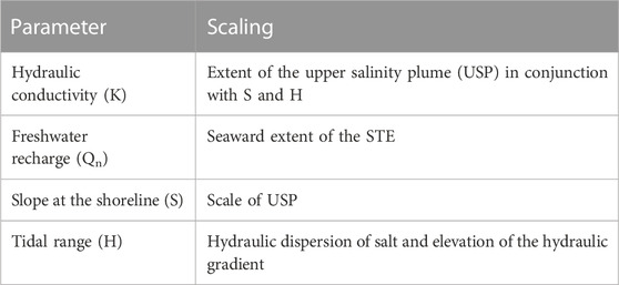
TABLE 1. Fundamental parameters of an STE typology.

5 An aside on STEs in earth history and climate change

Over geologic time spans, STEs probably exert a broader and more persistent impact on the oceans than their open-water kin. Open-water estuaries are ephemeral dependent on protected features of the configuration of the coastline. The lifetime of an open-water estuary may be only a few tens of thousands of years (Schubel and Hirschberg 1978). They are subject to infilling and relatively rare during periods of low stands of sea level. STEs, on the other hand, would enjoy a continuous existence everywhere along the shoreline (e.g., Metcalf et al., 2021), waxing and waning in importance only with global changes in shoreline length In the face of global warming and sea-level rise, open water estuaries would be expected to increase in importance. Changes in the elevation of sea level and the extent of glacial ice, STEs have been shown to migrate across the shelf far from shore (e.g., Roy et al., 2010; Hong et al., 2019; Liljedahl et al., 2021; Moore and Joye, 2021). The importance of STEs to deliver dissolved nutrients, carbon, hydrogen sulfide and other trace gasses, reduced metals, and radionuclides (Moore, 2010) would increase also as the shoreline length increases due to inundation and, perhaps, increases in freshwater recharge.

6 Conclusion

STEs might be considered just another type of estuary as defined for open-water estuaries, except for any difficulties posed by the “semi-enclosed” condition and the limits of the low Reynolds number approximation of the Navier-Stokes equation which requires the dominant position of permeability. With this in mind, a limited typology for STEs basically requires at least four parameters. These are the recharge, and the hydraulic conductivity, the slope of the coast and the tidal range, all of which are fundamental scaling factors for the salinity structure of the STE. Day, 1980, Fairbridge, 1980.

Data availability statement

The original contributions presented in the study are included in the article/supplementary material, further inquiries can be directed to the corresponding author.

Author contributions

The author confirms being the sole contributor of this work and has approved it for publication.

Conflict of interest

The author declares that the research was conducted in the absence of any commercial or financial relationships that could be construed as a potential conflict of interest.

Publisher’s note

All claims expressed in this article are solely those of the authors and do not necessarily represent those of their affiliated organizations, or those of the publisher, the editors and the reviewers. Any product that may be evaluated in this article, or claim that may be made by its manufacturer, is not guaranteed or endorsed by the publisher.

Footnotes

¹This might be analogous to hypersaline estuaries, also known as negative or reverse estuaries (Day 1980). An inverted estuarine density gradient can occur when evaporation is much larger than the freshwater supply.

²I am indebted to the scholarship of Carlos Rocha and Issac Santos for identifying Marcus Terentius Varro to be credited with defining an estuary as a place where the tides goes in as well as comes out, explicitly stated by Pompeius Festus in 150 A.DS. and later referred to in Pliny’s Natural History and in Ceasar’s Galllic Wars.

³A flow of low Reynolds Number is dominated by viscosity The Navier-Stokes equation is a partial differential equation that describes the flow of incompressible fluids, in this case, fluids of high viscosity where inertial forces can be neglected.

⁴Although in open water estuaries and in STEs too, the tides can reach far beyond the head of salt into freshwater, only the mixing zone is relevant here.

⁵To some extent, surface-water waves would also contribute in the same way to the critical hydraulic dispersion, although the impact would be more limited in extent due to the shortness of wave periods.

References

Anonymous, (1959). Venice 8014 April1958. Archivio di Oceanografe e Limnologieu 11 Supplemento (Simposio sulla Classificazione della Acque Salmastre).Symposium on the classification of brackish waters

Google Scholar

Athanasiou, P., van Dongeren, A., Giardino, A., Vousdoukas, M., Gaytan-Aguilar1, S., and Ranasinghe, R. (2019). Global distribution of nearshore slopes with implications for coastal retreat. Earth Syst. Sci. Data 11, 1515–1529. doi:10.5194/essd-11-1515-2019

CrossRef Full Text | Google Scholar

Bokuniewicz, H., Buddemeier, R., Maxwell, B., and Smith, C. (2003). The Typological Approach to submarine groundwater discharge (SGD). Biogeochemistry 66, 145–158. doi:10.1023/b:biog.0000006125.10467.75

CrossRef Full Text | Google Scholar

Bokuniewicz, H. (2001). Toward a coastal ground-water typology. J. Sea Res. 46, 99–108. doi:10.1016/s1385-1101(01)00074-0

CrossRef Full Text | Google Scholar

Boufadel, M. C. (2000). A mechanistic study of nonlinear solute transport in a groundwater surface water system under steady-state and transient hydraulic conditions. Water Resour Research 36, 2549–2565. doi:10.1029/2000wr900159

CrossRef Full Text | Google Scholar

Bulger, A. J., Hayden, B. P., Monaco, M. E. P. M. Nelson, McCormick-Ray, M. G., and Nelson, D. M. (1993). Biologically-based estuarine salinity zones derived from a multivariate analysis. Estuaries 16, 311–322. doi:10.2307/1352504

CrossRef Full Text | Google Scholar

Cooper, H. H. (1964). “Salt water in coastal aquifers, in sea water in coastal aquifers,” in U.S. Geological survey water supply Paper1613C: C1-C12. Editors H. Cooper, F. Kohout, H. Henry, and R. Glover (Reston, VA, USA: U.S. Geological Survey).

Google Scholar

Day, J. H. (1980). What is an estuary, South African Journal of Science, 76, 168.

Google Scholar

Doulgeris, C., Tziritis, E., Pisinaras, V., Papagopoulosu, A., and Kulls, C. 2020. Prediction of seawater intrusion into coastal aquifers based on non-dimensional diagrams. Available at https://www.lri.swri.gr/images/News/EGU/EGU2020_Charalampos_Doulgeris2.pdf accessed April 2021, SWRI. San Antonio, Texas, USA

Google Scholar

Fairbridge, R. W. (1980). “The estuary. Its definition and geodynamic cycle,” in Chemistry and bio-geochemistry of estuaries. Editors E. Olausson, and I. Caf (Texas, USA: Eureka Mag), 1–35.

Google Scholar

Geng, X., and Boufadel, M. (2015). Numerical study of solute transport in shallow beach aquifers subjected to waves and tides. J. Geophys. Res. Oceans 120, 1409–1428. doi:10.1002/2014jc010539

CrossRef Full Text | Google Scholar

Gleeson, T., Smith, L., Moosdorf, N., Hartman, J., Durr, H. H., Manning, A. H., et al. (2011). Mapping permeability over the surface of the Earth. Geophys. Res. Lett. 38 (6), L02401. doi:10.1029/2010GL045565

CrossRef Full Text | Google Scholar

Glover, R. E. (1964). “The pattern of fresh-water flow in a coastal aquifer in Sea Water in coastal aquifers,” in U.S. Geological survey water supply paper 1613-C: C32 – C35 (Reston, VA, USA: U.S. Geological Survey).

Google Scholar

Gosink, J. P., and Baker, G. C. (1990). Salt fingering in subsea permafrost-some stability and energy considerations. J. Geophys. Research-Oceans 95, 9575–9583. doi:10.1029/jc095ic06p09575

CrossRef Full Text | Google Scholar

Grezlac, K., Tamborski, J., and Bokuniewicz, L. Kotwick, H. (2018). Ecostructuring of marine nematode communities by submarine groundwater discharge. Mar. Environ. Res. 136, 106–119. doi:10.1016/j.marenvres.2018.01.013

PubMed Abstract | CrossRef Full Text | Google Scholar

Hansen, D. V., and Rattray, M. (1966). New dimensions in estuary classification. Limnol. Oceanogr. 11, 319–326. doi:10.4319/lo.1966.11.3.0319

CrossRef Full Text | Google Scholar

Hong, W. L., Lepland, A., Himmler, T., Kim, J.-H., Chand, S., Sahy, D., et al. (2019). Discharge of meteoric water in the eastern Norwegian Sea since the last glacial period. Geophys. Res. Lett. 46, 8194–8204. doi:10.1029/2019GL084237

CrossRef Full Text | Google Scholar

Ketchum, B. H. (1951). The flushing of tidal estuaries. Sew. Ind. Wastes 23, 198–209.

Google Scholar

Kirezci, E., Young, I. R., Ranasinghe, R., Muis, S., Nicholls, R. J., Lincke, D., et al. (2020). Projections of global-scale extreme sea levels and resulting episodic coastal flooding over the 21st Century. Sci. Rep. 10, 11629. doi:10.1038/s41598-020-67736-6

PubMed Abstract | CrossRef Full Text | Google Scholar

Knee, K., and Paytan, A. (2011). Submarine groundwater discharge: A source of nutrients, metals, and pollutants to the coastal ocean. Treatise Estuar. Coast. Sci. 4, 205–233.

Google Scholar

Kohout, F. A. (1960). Cyclic flow of saltwater in the Biscayne aquifer of southeastern Florida. J. Geophys. Res. 65, 2133–2141. doi:10.1029/jz065i007p02133

CrossRef Full Text | Google Scholar

Kotwicki, L., Grezlak, K., Czub, M., Dellwig, O., Gentz, T., and Szymczycha, B. (2014). Submarine groundwater discharge to the Baltic coastal zone: Impacts on the meiofaunal community. J Mar Syst 129, 118–126. doi:10.1016/j.jmarsys.2013.06.009

CrossRef Full Text | Google Scholar

Liljedahl, L. C., Meierbachtol, T., Harper, J., van As, D., Näslund, J. O., and Selroos, J. O., (2021). Rapid and sensitive response of Greenland’s groundwater system to ice sheet change. Nat Geosci 14, 751–755. doi:10.1038/s41561-021-00813-1

CrossRef Full Text | Google Scholar

Lyell, C. (1834). Principles of geology, Being Inq How Far Former Changes Earth’s Surface Referable Causes Now Operation Murray Lond, 4.

Google Scholar

McHugh, J. L. (1967). Editor G. H. Estuaries (Washington, DC, USA: American Association for the Advancement of Science), 83, 581–620.Estuarine nekton

Google Scholar

Metcalf, W. L., Bokuniewicz, H., and Terchunian, A. (1995). Water-table variations on a reflective ocean beach: Quogue, New York. Northeast. Geol. Environ. Sci 17, 61–67.

Google Scholar

Micallef, A., Person, M., Berndt, C., Bertoni, C., Cohen, D., Dugan, B., et al. (2021). Offshore freshened groundwater in continental margins. Rev Geophys 59, e2020RG000706. doi:10.1029/2020rg000706

CrossRef Full Text | Google Scholar

Miller, D. C., and Ullman, W. J. (2004). Ecological consequences of ground water discharge to Delaware bay, United States. U S Groundw 42, 959–970. doi:10.1111/j.1745-6584.2004.tb02635.x

CrossRef Full Text | Google Scholar

Mohan, C., Western, A. W., Wei, Y., and Saft, M. (2018). Predicting groundwater recharge for varying land cover and climate conditions – A global meta-study. Hydrology Earth Syst Sci 22, 2689–2703. doi:10.5194/hess-22-2689-2018

CrossRef Full Text | Google Scholar

Moore, W. S., and Joye, S. B. (2021). Saltwater intrusion and submarine groundwater discharge: Acceleration of biogeochemical reactions in changing coastal aquifers. Front. Earth Sci. 9, 600710. doi:10.3389/feart.2021.600710

CrossRef Full Text | Google Scholar

Moore, W. S. (2010). The effect of submarine groundwater discharge on the ocean. Annu. Rev. Mar. Sci. 2, 59–88. doi:10.1146/annurev-marine-120308-081019

PubMed Abstract | CrossRef Full Text | Google Scholar

Nielsen, P. (1990). Tidal dynamics of the water table in beaches. Water Resour. Res. 26, 2127–2134. doi:10.1029/wr026i009p02127

CrossRef Full Text | Google Scholar

Oz, I., Shalev, E., Yechieli, Y., and Gvirtzman, H. (2015). Saltwater circulation patterns within the freshwater-saltwater interface in coastal aquifers: Laboratory experiments and numerical modeling. J. Hydrology 530, 734–741. doi:10.1016/j.jhydrol.2015.10.033

CrossRef Full Text | Google Scholar

Perillo, G. M. E. (1995). “Definitions and geo-morphologic classifications of estuaries. In geomorphology and sedimentology of estuaries,”. Editor G. M. E. Perillo, 53, 17–47.Dev. Sedimentology

CrossRef Full Text | Google Scholar

Prieto, C., and Destouni, G. (2005). Quantifying hydrological and tidal influences on groundwater discharges into coastal waters. Water Resour. Res 41, W12427. doi:10.1029/2004WR003920

CrossRef Full Text | Google Scholar

Pritchard, D. W. (1960). Lectures on estuarine oceanography. B. Kinsoman. Baltimore, MD, USA: J. Hopkins University, 154. 298 ed.

Google Scholar

Robinson, C., Gibbes, B., Carey, H., and Li, L. (2007). Salt-freshwater dynamics in a subterranean estuary over a spring-neap tidal cycle. J. Geophys. Res. 112, C09007. doi:10.1029/2006jc003888

CrossRef Full Text | Google Scholar

Robinson, C., Gibbes, B., and Li, L. (2006). Driving mechanisms for groundwater flow and salt transport in a subterranean estuary. Geophys. Res. Lett. 33, L03402. doi:10.1029/2005GL025247

CrossRef Full Text | Google Scholar

Rocha, C., Robinson, C. E., Santos, I. R., Waska, H., Michael, H. A., and Bokuniewicz, H. J. (2021). A place for subterranean estuaries in the coastal zone. Estuar. Coast. Shelf Sci. 250, 107167. doi:10.1016/j.ecss.2021.107167

CrossRef Full Text | Google Scholar

Roy, M., Martin, J. B., Cherrier, J., Cable, J. E., and Smith, C. G. (2010). Influence of sea level rise on iron diagenesis in an east Florida subterranean estuary. Geochimica Cosmochimica Acta 74, 5560–5573. doi:10.1016/j.gca.2010.07.007

CrossRef Full Text | Google Scholar

Schubel, J. R., and Hirschberg, D. J. (1978). “Estuarine graveyards: Climate change and the importance of the estuarine environment,” in Proceedings of the fourth international estuarine research federation conference. Editors Estuarine Interactions, and M. Wiky (CA, USA: Academic Press), 285–303.

CrossRef Full Text | Google Scholar

Silva, A. C. E., Tavares, P., Shapouri, M., Stigter, T. Y., Monteiro, J. P., Machado, M., et al. (2012). Estuarine biodiversity as an indicator of groundwater discharge. Coast. Shelf Sci. 97, 38–43. doi:10.1016/j.ecss.2011.11.006

CrossRef Full Text | Google Scholar

Valiela, I., Costa, J., Foreman, K., Teal, J. M., Howes, B., and Aubrey, D. (1990). Transport of groundwater-borne nutrients from watersheds and their effects on coastal waters. Biogeochemistry 10, 177–197. doi:10.1007/bf00003143

CrossRef Full Text | Google Scholar

Williams, T., Amatya, D., Conner, W., Panda, S., Xu, G., Dong, J., et al. (2019). “Chapter 6, tidal forested wetlands: Mechanisms,threats, and management tools,”. Editors S. An, and J. T. A. Verhoeven, 238. doi:10.1007/978-3-030-14861-4_6Wetl. Ecosyst. Serv. Restor. Wise Use, Ecol. Stud.

CrossRef Full Text | Google Scholar

Zamrsky, D., Oude Essink, G. H., and Bierkens, M. F. (2018). Estimating the thickness of unconsolidated coastal aquifers along the global coastline. Earth Syst. Sci. Data 10, 1591–1603. doi:10.5194/essd-10-1591-2018

CrossRef Full Text | Google Scholar