Estimating P- and S-Wave Velocities in Fluid Mud Using Seismic Interferometry

Introduction

The geotechnical behavior of fluid mud significantly affects the navigability in ports and waterways. Better understanding of the geotechnical behavior of the fluid mud can thus help to estimate accurately the nautical depth and thus safe navigating through fluid mud, as well as decrease the dredging costs (McAnally et al., 2007; McAnally et al., 2016; Kirichek et al., 2018). The strength of the fluid mud is low but could increase over time due to the consolidation effect to form a layer with high rigidity (Abril et al., 2000). Port authorities usually have their own methods to determine the navigability of the fluid mud. For example, the Port of Rotterdam uses the levels of 1.2 kg/L while the Port of Emden uses the yield stress of 100 Pa as criteria for estimating the water/mud interface (Kirichek et al., 2018). These levels are chosen based on the combination of seismic data and yield stress/density vertical profiles, which are measured in a water/mud column by mud profilers (Kirichek et al., 2020; Kirichek and Rutgers 2020). Because of the individual differences in mud composition, an accurate parameter that can be adopted by different ports is needed. It is challenging to accurately measure the in-situ geotechnical behaviors of the fluid mud, because the common techniques of measurement, including yield strength and density measurement, will inevitably disturb the fluid mud during the intrusive sampling process (Kirichek et al., 2020). That is, why, a laboratory protocol was developed to determine the fluidic yield stresses (Shakeel et al., 2020). On the basis of this protocol, a link was found between the S-wave velocities and the fluidic yield stress (Ma et al., 2021). The non-intrusive measurements such as x-ray and ultrasonic measurements are favorable because other measurements will alter the characteristic of the fluid mud and the result will be inaccurate (Kirichek et al., 2018; Carneiro et al., 2020).

The ultrasonic measurements for fluid mud include transmission measurements and reflection measurements. The transmission measurements are straightforward and simple to use in a laboratory. In recent years, most commonly used seismic survey techniques for marine sediment, such as sonar and velocimeter, employ longitudinal (P-) waves (Gratiot et al., 2000; Schrottke et al., 2006). In a marine seismic survey, the sources and receivers need to be located in the water column. In practice, they are often close to the water surface, meaning that the sources, such as airgun arrays, and the receivers, usually towed by a vessel as streamers, send and receive only P-waves, respectively. Therefore, the utilization of S-waves is limited in the marine environment and extracting the S-wave information is challenging and time-consuming (Drijkoningen et al., 2012). At the same time, P-waves are related to the bulk properties of the materials and the geotechanical properties of marine sediments cannot be inferred only from P-waves. S-waves can be used to precisely characterize the fluid mud as the propagation velocity and amplitude of the S-waves strongly depend on the geotechanical properties of the marine sediments (Meissner et al., 1991). Developing an accurate and reliable way of using S-waves for the seismic survey in a marine environment without the complications of deploying receivers at the water bottom to characterize the marine sediments can greatly facilitate the investigation of the geotechnical behavior of the marine sediments. Leurer (2004), Ballard et al. (2014), Ballard and Lee (2016) performed transmission measurement in a laboratory to measure the velocities of the seismic waves. Leurer (2004) used high frequencies and found that the S-wave velocities ranged from 450 to 975 m/s. The S-wave velocity is calculated using travel distance and traveltime along the travelpath, which usually is a straight line (Ma et al., 2021). However, there are limitations using the transmission measurements in the field because there are no open side positions to plant the transducers as used in containers in the laboratory-measurement setup. In contrast, reflection measurements in marine exploration allow deploying the transducers or hydrophones in the water column. Using such measurements, layer-specific propagation velocities of the fluid mud can be estimated to monitor the variation of the shear strength of the fluid mud. Given that correlations are found between the S-wave velocity and the yield strength, the S-wave velocity can be used as a proxy to estimate the yield strength of the fluid mud; therefore, ultrasonic measurements have a great potential in helping estimate the yield strength of the fluid mud (Ma et al., 2021).

The goal of this study is to measure the layer-specific propagation velocities and investigate the temporal variation of these velocities with the consolidation of the fluid mud using seismic reflection measurement and retrieval of layer-specific reflections. To obtain the latter, we apply seismic interferometry (SI) to the recorded reflection data to eliminate the travelpaths inside the water layer and retrieve reflections only inside the fluid-mud layer. SI is a technique to retrieve new seismic recordings between receivers from cross-correlation of existing recordings at the receivers (e.g., Shapiro and Campillo 2004; Wapenaar and Fokkema 2006; Draganov et al., 2009; Draganov et al. 2010; Draganov et al. 2012; Draganov et al. 2013). In this study, we first briefly introduce the reflection measurements. We, then, show the process of retrieving seismic traces based on ghost-reflection retrieval, followed by the velocity-calculation process. We show the temporal variation of the propagation velocity inside the fluid-mud layer and the correlation between the S-wave velocities and yield strengths. Additionally, we compare the S-wave velocities from the reflection measurement to those of a transmission measurement that was performed in a previous study (Ma et al., 2021).

Materials and Methods

We have developed a seismic reflection system to measure the layer-specific propagation velocities. Below, we give a short description of the main measurement steps. The sample and the system are described in detail in Ma et al. (2021). The mud sample was retrieved from the Calandkanaal (Port of Rotterdam). The sampling location is shown in Figure 1A. Before the reflection measurement, a two-layer system is formed due to the density difference between water and fluid mud (Figures 1C,D). We first stir the fluid mud using a mechanical mixer to ensure that the fluid mud is in a homogeneous form with a uniform density (Figure 1B). We deposit the fluid mud in the fluid-mud tank and gently add water above it without eroding the fluid-mud layer in the tank. The fluid mud in the tank settles and consolidates during the self-weight consolidation process. At the start of the measurements, the water layer is about 82 mm thick, the mud layer below it is about 100 mm thick.

FIGURE 1

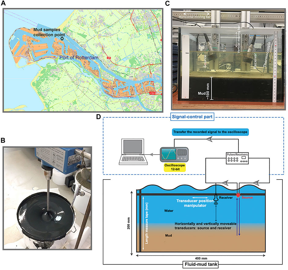
FIGURE 1. (A) Mud-samples collection location in the Calandkanaal (Port of Rotterdam). (B) Mud-stirring process using a mechanical mixer. (C) A glass tank with fluid mud, transducers, and a thermocouple. (D) A cartoon showing the reflection measurement system.

The Reflection Measurement System

The reflection measurement system includes a signal control part, a fluid-mud tank, and ultrasound transducers (Figure 1D). We use a transparent glass tank that allows to visually see the settlement of the fluid-mud layer (Figure 1C). The multiple positions of the receiver transducer along the horizontal direction are evenly distributed so that a common-source gather (CSG) can be constructed by placing one after the other the measurements (traces) at each consecutive horizontal position of the receiver. The horizontal distance between the receiver positions is 5 mm. The distance between the first and last receiver positions, which correspond to the shortest and longest source-receiver offsets, respectively, is 95 mm, meaning that a CSG includes 20 traces at different offsets. The parameters of the acquisition geometry and the different kinds of expected arrivals for this two-layer system are shown in Figure 2. For our analysis, we use the P-wave reflection of the mud top and the primary reflections of the mud bottom (explained in the following section).

FIGURE 2

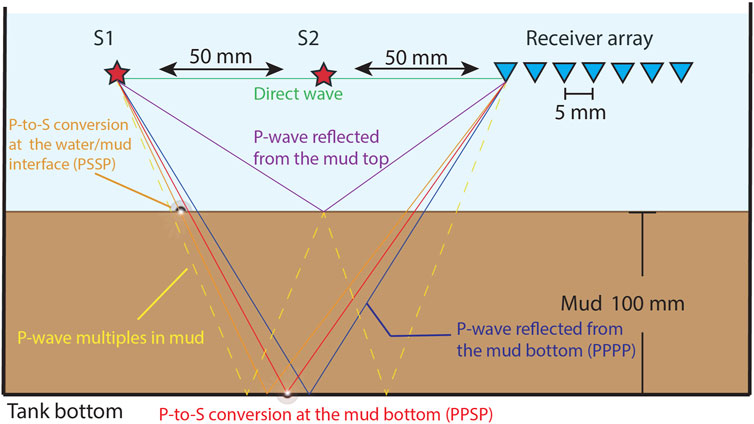
FIGURE 2. Illustration of the acquisition geometry and different kinds of arrivals expected to be recorded in a reflection measurement. The receiver array illustrates only the first seven receiver; the proportions are exaggerated; the paths through the water/mud interface are shown as straight lines for illustration purposes.

Time-Lapse Measurement and Data Acquisition

We place the source transducer at two positions, labeled S1 and S2 in Figure 2, the signals of which are recorded by the same receiver array. The sources are distanced 50 mm and 100 from the leftmost receiver. The excitation frequency of the sources is 100 kHz. By applying SI to the recordings from the two sources at a specific receiver position to retrieve a ghost source and a ghost receiver that are effectively placed on the top of the mud, i.e., the water/mud interface (Figure 3). Cross-correlating the reflection from the mud top with the reflection from the mud bottom effectively eliminates the common travelpath from S1 to the receiver and S2 to the receiver in the water layer (dashed lines in Figure 3). Because the specific receiver position depends on the thickness and velocity of the mud layer, and thus changes with time, we record CSGs.

FIGURE 3

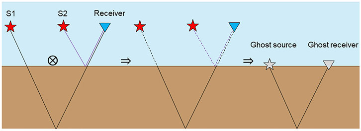
FIGURE 3. Sketch of the retrieving a ghost reflections using seismic interferometry by correlating two traces that effectively eliminates the common travelpaths in the water layer (dashed lines).

We monitor the changes in the propagation velocities in the two-layer system during a 2-week period. During several days in this period, we conduct measurements to obtain a CSG from each source. In the first week, we perform reflection measurements every day from Monday to Friday. In the second week, we only conduct a reflection measurement on Friday. As shown in Figure 4, there are two kinds of primary reflections that we emphasize in this study. One kind is the arrival that is, reflected by the mud top (Figure 4A). The other kind are the arrivals that are reflected by the mud bottom (Figures 4B–D). The latter represents three reflections with different travelpaths according to their possible partial conversions. During the propagation of the P-wave originating from the source transducer, part of the energy propagates as a P-wave along the complete downward and upward travelpaths (Figure 4B). A part of the energy converts to an S-wave when the P-wave is reflected by the mud bottom (Figure 4C). Yet another part of the energy converts to an S-wave when the P-wave hits the water/mud interface and continues to propagate as such downward to the mud bottom and up to the water/mud interface (Figure 4D). In order to compute the propagation velocities of the P- and S-wave inside the fluid mud, we need to obtain the travel distances and traveltimes along the travelpaths within the fluid mud. However, the travelpaths of the primary reflections contain also the travelpaths inside the water, as shown in Figures 4B–D. Figure 4B illustrates the travelpaths of the reflected P-wave which does not undergo any conversion (PP). In this way, the wave has the same incidence and reflection angle at the mud bottom and thus the downward and upward travelpaths are symmetrical. Figures 2, 4C shows the travelpaths of the reflected P-wave that converts to an S-wave after reflecting at the mud bottom (PPSP). Due to conversion, the incidence and reflection angle are different and thus the downward and upward travelpaths are asymmetrical. As shown in Figures 2, 4D, the P-wave also converts to an S-wave when hitting the water/mud interface and the S-wave converts again to a P-wave only at the water/mud interface along the upward travelpath (PSSP). Because of this, the downward and upward travelpaths are symmetrical. Note that the primary reflection PSPP has an identical arrival time as the PPSP primary for a laterally homogeneous medium, the PPSP arrival essentially is the superposition of both PPSP and PSPP. In Figures 2, 4C, we only illustrate the PPSP travelpaths. From here on, we only use the label PPSP but we understand the superposition of PPSP and PSPP.

FIGURE 4

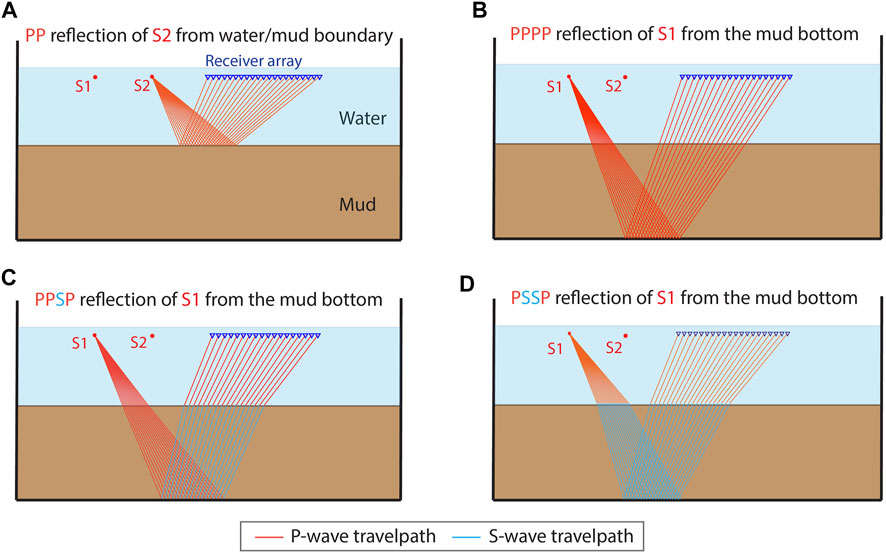
FIGURE 4. Travelpaths of the primary reflections in the ultrasonic reflection measurement: (A) the P-wave reflection (PP) from the water/mud interface from source S2; (B) the P-wave reflection (PPPP) from the bottom of the mud layer from source S1; (C) the reflection from the bottom of the mud layer partly converted to an S-wave (PPSP) from source S1; (D) the reflection from the bottom of the mud layer completely converted to an S-wave (PSSP) from source S1. The primary reflection in (A) is used to correlate with the primary reflections in (B–D).

We apply the SI method for retrieval of ghost reflections. For this, we correlate trace-by-trace the PP reflection arrivals in the CSG from source S2 (Figure 4A) with each of the three primary reflection arrivals, i.e., PPPP, PPSP, and PSSP, in the CSG from source S1 (Figures 4B–D). The results are three correlation gathers containing correlated traces. The final step of SI is the summation of the traces inside each of the three correlation gathers. In this way, we retrieve three ghost reflections that appear to have propagated only inside the fluid-mud layer by effectively removing the travelpaths inside the water layer. These three ghost reflections represent a PP, PS, and SS reflection arrivals. Next, we pick the two-way traveltimes of the ghost reflection inside the fluid mud and calculate the travel distances along the travelpaths. Calculation of the travel distances is possible as the distance between the source and receiver of the three ghost reflections is always the same and equal to the distance between the sources S1 and S2, while we monitor the thickness of the fluid-mud layer using a ruler along the vertical wall of the tank. We then estimate the P- and S-wave velocities in the fluid-mud layer by dividing the travel distance by the picked two-way traveltimes While the calculations for the PP and SS ghost reflections are straightforward, to calculate the velocities from the PS ghost reflection, we form a system of three equations with three unkowns $x, y, \text{and} v_s$:

$x+y=50(1)$

$\frac{sin\left(i\right)}{sin\left(r\right)}=\frac{x/d_p}{y/d_s}=\frac{v_p}{v_s}(2)$

$\frac{d_p}{v_p}+\frac{d_s}{v_s}=t_{two-way travel}(3)$

Equation 1 states that the distance between the ghost source and the ghost receiver is 50 mm, which is the sum of the horizontal projection x of the P-wave travelpath and y of the S-wave travelpath of the PS travelpath inside the fluid-mud layer (Figure 5). Eq. 2 is established based on the Snell’s law, where d_p is the P-wave travelpath, d_s is the S-wave travelpath, and $v_P \text{and} v_s$ are the velocities of the P- and S-wave inside the fluid-mud layer. Eq. 3 shows that the two-way traveltime is the sum of the traveltimes of P-wave and S-wave inside the layer. Additionally, h represents the thickness of the mud layer (Figure 5). As shown in Figure 5, $d_p=\sqrt{x^2+h^2}$ and $d_s=\sqrt{y^2+h^2}$. We consider $v_P$ known as we calculate it using the PP ghost reflection.

FIGURE 5

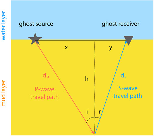
FIGURE 5. Geometry and parameters (see text for their explanation) for S-wave velocity calculation based on Snell’s law.

Results and Discussion

We record CSG from S1 and S2 on each of the days from Monday to Friday during the first week and on Friday during second week. Figure 6 shows the CSGs for days 0, 2, 4. The arrivals from S1 appear to be characterized by lower amplitudes than those from S2 which is expected because the receiver array is 50 mm closer to S2 compared to S1. The recording order in time of the different arrivals depends on the propagation velocities of the seismic waves in the water and fluid-mud layers and the travel distances along the travelpaths. The different arrival types we identify are color-coded in Figure 6. As we explained above, we aim to utilize the PP, PPPP, PPSP, and PSSP reflection arrivals to monitor for velocity changes during the 2-week self-weight consolidation. Although with the consolidation the two-way traveltime of the reflection arrivals PPP, PPSP, and PSSP gradually decreases, it is still uncertain whether the P- and/or S-wave velocities can increase because the thickness of the fluid-mud layer decrease due to the settling. The decrease of the two-way traveltime could result from decrease of the travel distance or from increase of the P- and/or S-wave velocities. Note that simultaneously with the decrease of the thickness of the fluid-mud layer, the thickness of the water layer increases. It is thus necessary to accurately calculate the velocities inside the fluid-mud layer using the travelpaths and two-way traveltimes of reflection arrivals from only inside the fluid mud. As we explain above, we achieve this using SI for retrieval of ghost reflections.

FIGURE 6

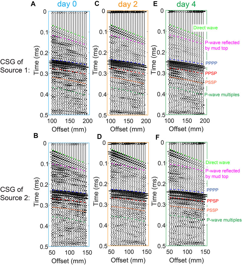
FIGURE 6. Common-source gathers (CSGs) for sources S1 (A, C, E) and S2 (B, D, F) for day (A, B) 0, (C, D) 2, (E, F) 4. The CSGs for days 1, 3, 11 are shown in Supplementary Appendix S1. The color coding indicates different arrivals.

Figures 6B,D,F show the interpreted direct waves and reflection arrivals from S2. The direct waves (light green color) interfere with the PP reflections (magenta color) from the fluid-mud top. In the SI process for retrieval of ghost reflections, we need to correlate the PP reflection from S2 with the primary reflections from the fluid-mud bottom from S1—PPPP, PPSP, and PSSP. In order to suppress the influence of the direct waves on the PP reflections, we use a frequency-wave number filter (Ma et al., 2021). After the correlation, we obtain correlation gathers (left columns in Figures 7A,B), which we have to sum along the receiver positions to obtain the final retrieved ghost reflections. As shown in Ma et al. (2021), more accurate retrieval is obtained when summing only the traces inside the so-called stationary-phase region (Snieder, 2004). In the summation process, such traces contribute constructively to the final result, while traces outside the stationary-phase region should interfere destructively with each other if sufficiently long receiver array is available. AS our array is limited in length, we taper the traces outside the stationary-phase region. The results of the summations (right columns in Figures 7A,B) represent retrieved ghost reflections with travelpaths only inside the fluid-mud layer. In Figure 7, we show the retrieved ghost reflections PP and PS. The ghost reflections SS are not included in this study because the energy of the PSSP reflections is relatively lower when the settling time is not long enough, making the retrieval of SS for the earlier days difficult. Longer settling time causes a larger difference between the densities of the water and the fluid mud meaning that a greater portion of the P-wave energy turns into S-wave energy when stricking the water/mud interface. Only the measurement after 1 week can ensure an accurate pick and reliable retrieval for the ghost reflection SS, the result of which was presented in Ma et al. (2021). So, in this study, we calculate S-wave velocities from the retrieved ghost reflections PS. We then use the retrieved ghost reflections to pick the first break to determine the two-way traveltime of these arrivals (green numbers in the right columns in Figure 7). We do the same also for days 1, 3, and 11 (see figures in Supplementary Appendix SA).

FIGURE 7

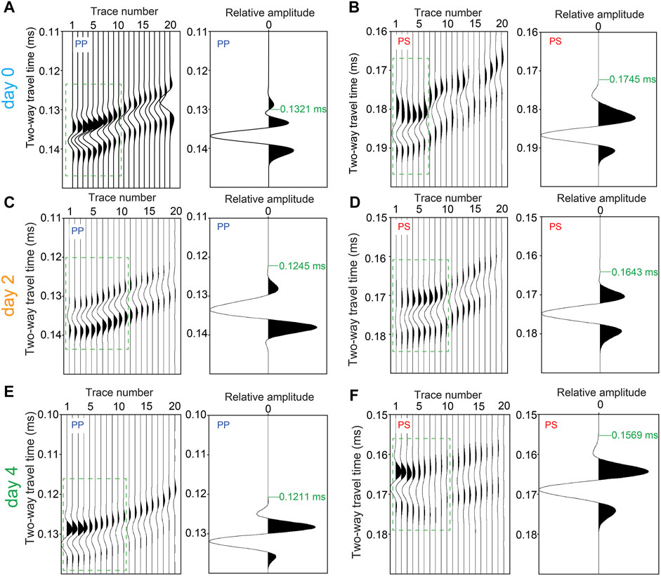
FIGURE 7. Correlation gathers (left columns) and retrieved ghost reflections (right columns) from inside the fluid-mud layer for (A, B) day 0, (C, D) day 2, and (E, F) day 4. The results in the right columns are obtained by summing the traces inside stationary-phase region (the green rectangles) in the corresponding left columns. (A, C, E) Retrieval of PP ghost reflections. (B, D, F) Retrieval of PS ghost reflections. The green numbers in the right columns indicate the picked arrival times of the retrieved ghost reflections.

Using the picked two-way traveltimes, we can estimate the P- and S-wave velocities using the travelpath distances. Figure 8 shows the PP and PS travelpath distances for day 0. The travelpath of PP is symmetrical so that the travel distances for the left leg and the right leg are equal. In contrast, the travelpath of PS is asymmetrical, and thus the travel distances of the left leg for the P-wave and the right leg for the S-wave need to be calculated by solving the system of Eqs 1–3 using the two-way traveltime pick and the known P-wave velocity from the ghost reflection PP. Here, we calculate the velocities using the parameters from Table 1 for day 0. The P-wave velocity is estimated to be 1,590 m/s. The S-wave velocity is thus estimated to be 966 m/s.

FIGURE 8

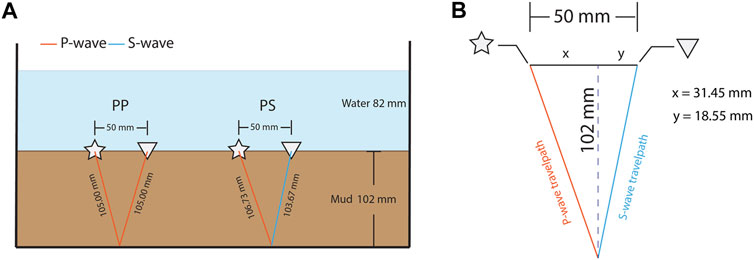
FIGURE 8. (A) The travelpath distances for ghost reflections PP and PS; (B) Illustration of the calculation for the unsymmetrical travelpath of PS.

TABLE 1

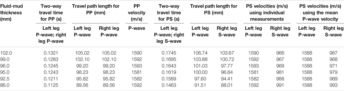
TABLE 1. Parameters for calculating the P- and S-wave velocities inside the fluid-mud layer for the six different days of measurements.

Using the same process, we analyze the seismic traces of the measurement from day 0 to day 11 and monitor the time-lapse evolution of the P- and S-wave velocities (Table 1). For comparison, Table 1 also includes the S-wave velocities estimated using the mean P-wave velocity from the reflection measurement. The S-wave velocities estimated using the mean P-wave velocity and the individual P-wave velocities are very close to each other. As shown in Table 2, the P-wave velocities suggest that, although we observe fluctuations, there is no obvious pattern for P-wave velocity change in relation to the consolidation. On the other hand, the S-wave velocities appear to be clearly increasing with the consolidation process, despite the apparent close velocities for day 0 and day 1.

TABLE 2

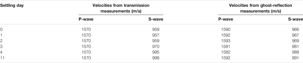
TABLE 2. Time-lapse velocities from transmission and the ghost-reflection measurements.

Additionally, we synchronously measure the yield stress of the fluid mud using a rheometer with Couette geometry and Vane geometry. We compare the progress of the fluidic yield stress with consolidation and examine the correlation with the S-wave velocities. As shown in Figure 9, the S-wave velocities (green dots; calculated using the P-wave velocities estimated from the PP ghost reflection for each day) appear to be positively correlated with the fluidic yield stress with the progress of the consolidation for both the reflection measurement in this study and the transmission measurements (blue dots) from Ma et al. (2021). The overall change of the S-wave velocities with the evolution of the fluidic yield stress indicates a nonlinear process. From day 0 to day 2, although the fluidic yield stress shows a pronounced increase, the S-wave velocities show a limited increase, especially for the measurement with Vane geometry. This could be ascribed to the initial homogeneous status of the fluid mud. We start the measurements after homogenizing the fluid mud. The conversion from the homogeneous to inhomogeneous condition could certainly strengthen the fluidic yield stress of the fluid mud. However, during the conversion from homogeneous to inhomogeneous mud, the effect of the consolidation probably cannot contribute to the immediate increase of the S-wave velocities. From day 2 to day 3, the S-wave velocities notably increase with a mild rise of the fluidic yield stress. This implies that the S-wave velocities are more sensitive to the increase of the yield stress when the consolidation has started with a duration more than 24 h. From day 2 to the last day—day 11, the correlation between the S-wave velocities and the fluidic yield stress shows a good apparently linear relationship. The measurements from day 2 to day 11, which are within the linear increase duration, show that the average increase rate of the fluidic yield stress is 1.84 m/(s*Pa) with the Couette geometry and is 1.03 m/(s*Pa) with the Vane geometry.

FIGURE 9

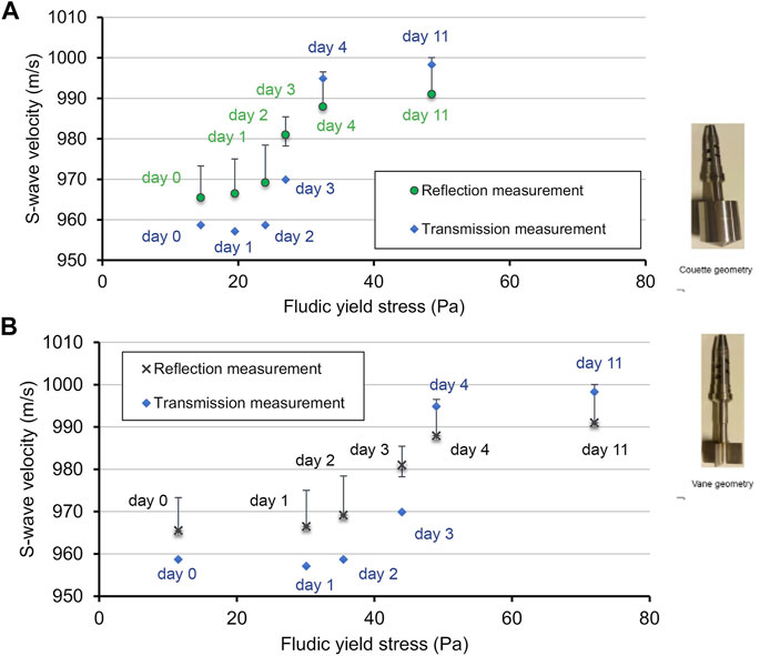
FIGURE 9. Evolution of the S-wave velocity (green dots) with the fluidic yield stress, where the latter is measured by (A) the Couette geometry and (B) the Vane geometry. The protocol to determine the fluidic yield stresses was developed by Shakeel et al. (2020). The black bars indicate the uncertainty interval. The uncertainty is estimated by taking the larger difference per day between the S-wave velocity estimated using the P-wave velocities from the corresponding daily ghost-reflection measurement and either the S-wave velocity estimated using the average of the P-wave velocities from the daily ghost-reflection measurements or the S-wave velocity estimated using the P-wave velocity from the transmission measurement. The transmission-measurement result is from Ma et al. (2021).

We also compare the estimated S-wave velocities from our ghost-reflection measurements with the S-wave velocities from seismic transmission measurements that were also conducted synchronously (Ma et al., 2021). The comparison in Table 2 shows that, the S-wave velocities from both the ghost-reflection and the transmission measurement are close but nevertheless they exhibit small differences. One reason for this could be that the directional difference of the seismic transmission measurement and the reflection measurement causes a discrepancy. In the transmission measurements, the source and the receiver transducers are mounted at the same height on opposite sides of the measurement tank, and thus the travelpath from the source transducer to the receiver transducer is along the horizontal direction. The seismic transmission measurement essentially sample the S-wave velocities horizontally along the middle part of the fluid-mud layer because the transducers were mounted there. In contrast, the waves in the reflection measurements travel the complete height of the fluid-mud layer twice along paths as in Figure 8. Thus, the two measurement geometries might be facing the effect of anisotropy between the horizontal and vertical directions. This means that the S-wave velocities estimated from the ghost reflections might reflect possible changes in consolidation with depth.

Another reason for differences in the S-wave velocities from the transmission and ghost-reflection measurements is that we estimate the S-wave velocities from the ghost reflections using the estimated P-wave velocities from the PP ghost reflections. Comparing the P-wave velocities estimated from the transmission and ghost-reflection measurements in Table 2; Figure 10, we see that they are also slightly different. An error in estimating the P-wave velocity might be coming from insufficient sampling of the stationary-phase region. Another error might be due to the differences in the directionality in the measurement geometries of the transmission and reflection measurements, just like for the S-waves. Still, the maximal error in the estimated P-wave velocities is 0.29%, which can ensure a reliable estimation of the S-wave velocities. To visualize this, we compare the estimated S-wave velocities using the estimated P-wave velocities from the PP ghost reflections for each of the 6 days of the measurements to the S-wave velocities estimated using the average P-wave velocity obtained by averaging the six individual PP ghost-reflection velocities. We show these results in the rightmost column in Table 1. As we can see, the differences are very small, i.e., less than 0.9%. We visualize the comparison also in Figure 9 by the black uncertainty intervals. We calculate the intervals for each measurement day: using the P-wave velocity averaged from the six individual PP ghost-reflection velocities and using the P-wave velocity from the transmission measurements; taking the maximum difference between the S-wave velocity for each measurement day and the S-wave velocity obtained using the average or transmission P-wave velocity; the maximum difference is assigned as the uncertainty interval. We can see that the uncertainly interval is again less than 0.9%.

FIGURE 10

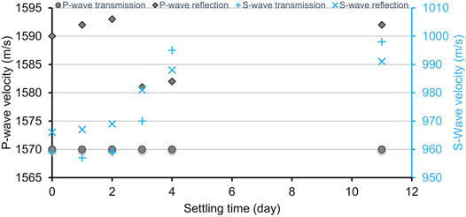
FIGURE 10. Comparison of P- and S-wave velocities from the transmission measurement in Ma et al. (2021) and the reflection measurement.

The results from our laboratory experiments show that using ghost reflections has a good potential for monitoring the seismic-velocity characteristics, and consequently also the fluidic yield stress, of fluid mud. Our experiment used fluid-mud layer with thickness of about 100 mm and source signals with center frequency of 100 kHz. We expect that this could upscaled to the field situation of a port or waterway with a thickness of the fluid-mud layer of about 2 m by using a source signal with a center frequency of 5 kHz as this would keep the same proportions relative to the dominant wavelengths in the fluid mud. The length of the acquisition geometry, which in our experiment had a maximum source-receiver offset of about 200 mm could be upscaled in the same way, i.e., relative to the thickness of the fluid-mud layer. An extra factor to take here into account is the thickness of the water layer. The length of an acquisition setup in a port or waterway should be such that the expected incidence angles at the water/fluid-mud interface are sufficiently away from vertical to allow P-to-S-wave conversions at the interface. I.e., the deeper the interface, the longer the maximum source-receiver offset. This would also entice assuming local lateral homogeneity in the water at the scale of the maximum source-receiver offset; inside the fluid-mud layer, the assumption for local lateral homogeneity would still be at the scale of the distance between the two source only.

Conclusion

We investigated longitudinal (P-) and transverse (S-) wave velocities in fluid mud for time-lapse monitoring of the geotechnical behavior of fluid mud in a water/fluid-mud system. For this, we used ultrasonic laboratory data from measurements in reflection geometry. We estimated P- and S-wave velocities directly from inside the fluid mud by removing the influence of the water layer by application of seismic interferometry for retrieval of ghost reflections. The latter allowed us to retrieve a P-wave reflection and a P-to-S-wave converted reflection from the bottom of the fluid mud as if from measurements with a source and receiver directly placed at the top of the fluid mud. We compared the estimated P- and S-wave velocities to values estimated from direct transmission measurements made horizontally along the middle height of the fluid-mud layer. The comparison showed that the transmission velocity of P-wave was more stable than the reflection velocity, which appeared to be fluctuated. The reflection S-wave velocity and the transmission S-wave velocity were close to each other. The S-wave velocities we estimated in the fluid-mud layer from the ghost reflections increase with the self-weight consolidation of the fluid mud, while the P-wave velocities did not show a trend. Concurrently, the yield stress of the fluid mud also increased with the consolidation. We found that the S-wave velocities are positively correlated with the fluidic yield stress of the fluid mud. This relationship implies that the time-lapse change in S-wave velocities might be used to indicate the progress of consolidation, which would provide a basis for a new non-intrusive ultrasound measurement tool in ports and waterways for monitoring the condition of the fluid mud.

Data Availability Statement

The original contributions presented in the study are included in the article/Supplementary Material, further inquiries can be directed to the corresponding author.

Author Contributions

XM: Conceptualization, Formal analysis, Investigation, Methodology, Validation, Visualization, Writing—original draft, Writing—review and editing. AK: Funding acquisition, Resources, Validation, Writing—review and editing, Supervision, Project administration. KH: Formal analysis, Investigation, Methodology, Validation. DD: Funding acquisition, Formal Analysis, Methodology, Resources, Writing—review and editing, Supervision, Project administration.

Funding

This research is supported by the Division for Earth and Life Sciences (ALW) with financial aid from the Netherlands Organization for Scientific Research (NWO) with grant no. ALWTW.2016.029.

Conflict of Interest

The authors declare that the research was conducted in the absence of any commercial or financial relationships that could be construed as a potential conflict of interest.

Publisher’s Note

All claims expressed in this article are solely those of the authors and do not necessarily represent those of their affiliated organizations, or those of the publisher, the editors and the reviewers. Any product that may be evaluated in this article, or claim that may be made by its manufacturer, is not guaranteed or endorsed by the publisher.

Acknowledgments

The project is carried out within the framework of the MUDNET academic network https://www.tudelft.nl/mudnet/. The authors thank Ahmad Shakeel for helping the rheological experiments and data analysis.

Supplementary Material

The Supplementary Material for this article can be found online at: https://www.frontiersin.org/articles/10.3389/feart.2022.806721/full#supplementary-material

References

Abril, G., Riou, S. A., Etcheber, H., Frankignoulle, H., De Wit, R., and Middelburg, J. J. (2000). Transient, Tidal Time-Scale, Nitrogen Transformations in an Estuarine Turbidity Maximum—Fluid Mud System (The Gironde, South-West France). Estuar. Coast. Shelf Sci. 50 (5), 703–715.

CrossRef Full Text | Google Scholar

Ballard, M. S., and Lee, K. M. (2016). Examining the Effects of Microstructure on Geoacoustic Parameters in fine-grained Sediments. The J. Acoust. Soc. America 140 (3), 1548–1557. doi:10.1121/1.4962289

CrossRef Full Text | Google Scholar

Ballard, M. S., Lee, K. M., and Muir, T. G. (2014). Laboratory P- and S-Wave Measurements of a Reconstituted Muddy Sediment with Comparison to Card-House Theory. J. Acoust. Soc. America 136 (6), 2941–2946. doi:10.1121/1.4900558

CrossRef Full Text | Google Scholar

Carneiro, J. C., Gallo, M. N., and Vinzón, S. B. (2020). Detection of Fluid Mud Layers Using Tuning Fork, Dual-Frequency Echo Sounder, and Chirp Sub-Bottom Measurements. Ocean Dyn. 1–18.

CrossRef Full Text | Google Scholar

Draganov, D., Campman, X., Thorbecke, J., Verdel, A., and Wapenaar, K. (2009). Reflection Images From Ambient Seismic Noise. Geophys. 74, A63–A67. doi:10.1190/1.3193529

CrossRef Full Text | Google Scholar

Draganov, D., Ghose, R., Heller, K., and Ruigrok, E. (2013). Monitoring Changes in Velocity and Q Using Non-physical Arrivals in Seismic Interferometry. Geophys. J. Int. 192, 699–709. doi:10.1093/gji/ggs037

CrossRef Full Text | Google Scholar

Draganov, D., Ghose, R., Ruigrok, E., Thorbecke, J., and Wapenaar, K. (2010). Seismic Interferometry, Intrinsic Losses andQ-Estimation. Geophys. Prospecting 58 (3), 361–373. doi:10.1111/j.1365-2478.2009.00828.x

CrossRef Full Text | Google Scholar

Draganov, D., Heller, K., and Ghose, R. (2012). Monitoring CO2 Storage Using Ghost Reflections Retrieved from Seismic Interferometry. Int. J. Greenhouse Gas Control. 11, S35–S46. doi:10.1016/j.ijggc.2012.07.026

CrossRef Full Text | Google Scholar

Drijkoningen, G., Allouche, N., Thorbecke, J., and Bada, G. (2012). Nongeometrically Converted Shear Waves in marine Streamer Data. Geophysics 77 (6), P45–P56. doi:10.1190/geo2012-0037.1

CrossRef Full Text | Google Scholar

Gratiot, N., Mory, M., and Auchere, D. (2000). An Acoustic Doppler Velocimeter (ADV) for the Characterisation of Turbulence in Concentrated Fluid Mud. Continental Shelf Res. 20 (12-13), 1551–1567. Sep 10. doi:10.1016/s0278-4343(00)00037-6

CrossRef Full Text | Google Scholar

Jackson, D., and Richardson, M. (2007). High-Frequency Seafloor Acoustics. Springer Science & Business Media.

Google Scholar

Kirichek, A., Chassagne, C., Winterwerp, H., and Vellinga, T. (2018). How Navigable Are Fluid Mud Layers. Terra Aqua: Int. J. Public Works, Ports Waterways Dev. 151.

Google Scholar

Kirichek, A., and Rutgers, R. (2020). Monitoring of Settling and Consolidation of Mud after Water Injection Dredging in the Calandkanaal. Terra et Aqua 160, 16–26.

Google Scholar

Kirichek, A., Shakeel, A., and Chassagne, C. (2020). Using In Situ Density and Strength Measurements for Sediment Maintenance in Ports and Waterways. J. Soils Sediments 20 (6), 2546–2552. doi:10.1007/s11368-020-02581-8

CrossRef Full Text | Google Scholar

Leurer, K. C. (2004). Compressional- and Shear-Wave Velocities and Attenuation in Deep-Sea Sediment during Laboratory Compaction. J. Acoust. Soc. America 116 (4), 2023–2030. doi:10.1121/1.1782932

CrossRef Full Text | Google Scholar

Ma, X., Kirichek, A., Shakeel, A., Heller, K., and Draganov, D. (2021). Laboratory Seismic Measurements for Layer-specific Description of Fluid Mud and for Linking Seismic Velocities to Rheological Properties. J. Acoust. Soc. America 149 (6), 3862–3877. Jun 3. doi:10.1121/10.0005039

CrossRef Full Text | Google Scholar

McAnally, W. H., Friedrichs, C., Hamilton, D., Hayter, E., Shrestha, P., and Rodriguez, H. (2007). Management of Fluid Mud in Estuaries, Bays, and Lakes. I: Present State of Understanding on Character and Behavior. J. Hydraul. Eng. 133 (1), 9–22.

CrossRef Full Text | Google Scholar

McAnally, W. H., Kirby, R., Hodge, S. H., Welp, T. L., Greiser, N., Shrestha, P., et al. (2016). Nautical Depth for US Navigable Waterways: A Review. J. Waterw. Port Coast. Ocean Eng. 142 (2), 04015014.

CrossRef Full Text | Google Scholar

Meissner, R., Rabbel, W., and Theilen, F. (1991). “The Relevance of Shear Waves for Structural Subsurface Investigations,” in Shear Waves in Marine Sediments (Dordrecht: Springer), 41–49.

CrossRef Full Text | Google Scholar

Schrottke, K., Becker, M., Bartholomä, A., Flemming, B. W., and Hebbeln, D. (2006). Fluid Mud Dynamics in the Weser Estuary Turbidity Zone Tracked by High-Resolution Side-Scan Sonar and Parametric Sub-bottom Profiler. Geo-mar Lett. 26 (3), 185–198. Sep 1. doi:10.1007/s00367-006-0027-1

CrossRef Full Text | Google Scholar

Shakeel, A., Kirichek, A., and Chassagne, C. (2020). Rheological Analysis of Mud from Port of Hamburg, Germany. J. Soils Sediments 20 (6), 2553–2562. doi:10.1007/s11368-019-02448-7

CrossRef Full Text | Google Scholar

Shapiro, N. M., and Campillo, M. (2004). Emergence of Broadband Rayleigh Waves from Correlations of the Ambient Seismic Noise. Geophys. Res. Lett. 31 (7). doi:10.1029/2004gl019491

CrossRef Full Text | Google Scholar

Snieder, R. (2004). Extracting the Green's Function from the Correlation of Coda Waves: a Derivation Based on Stationary Phase. Phys. Rev. E Stat. Nonlin Soft Matter Phys. 69 (4), 046610. doi:10.1103/PhysRevE.69.046610

PubMed Abstract | CrossRef Full Text | Google Scholar

Wapenaar, K., and Fokkema, J. (2006). Green's Function Representations for Seismic Interferometry. Geophysics 71 (4), SI33–SI46. doi:10.1190/1.2213955

CrossRef Full Text | Google Scholar