Adaptive Interpolation Method for Generalized Triangular Prism (GTP) Geological Model Based on the Geometric Smoothness Rule

Introduction

Recently, the development of human activities in underground spaces has gradually intensified. Due to the subsurface informationization basis, geology (Mansouri et al., 2015; Feizi et al., 2021), water conservancy (Oliveira et al., 2021), hydropower engineering (Bai and Tahmasebi, 2020), mines (Che and Jia, 2019), economic geology (Cuma et al., 2012), hydrology, underground engineering, city ground water, and many other subsurface fields are in urgent need of accurate geometric expressions of underground structures (Ghaleshahi et al., 2015). As a result, many true 3D geological modeling software are becoming a platform to show dynamically geometric structure shape and numerical analysis simulations of the subspace (Hodkiewicz, 2014; Jacquemyn et al., 2018).

Because of the core problem with 3D geological modeling, the researchers have carried out many works in the fields (Mansouri et al., 2015; Hillier et al., 2021). Currently, two expression methods are mainly used, the boundary expression model (BRep) (D’Affonseca et al., 2020) and the solid voxel model (Bai and Tahmasebi, 2020), while 3D spatial interpolation (Mei et al., 2016) is also used for calculating unknown locations with sparse data. The BRep method usually uses a triangular irregular network (TIN) (Watson et al., 2015) or a quadrilateral network as the base geometric voxel to express the external shape boundary of the geological body using discrete points. This method requires less storage with high calculation efficiency because it can only model the 3D outer boundary of the geological body, this is used in many 3D visualization applications. But unlike the voxel model, the BRep method cannot express the internal property, and the modeling source data are suitable for discrete points. However, the voxel model (Abdul-Rahman and Pilouk, 2008) uses tetrahedrons (Zehner et al., 2015),octrees (Fan et al., 2013), hexahedral grids (Caumon et al., 2005) and generalized triangular prism (GTP) (Wu, 2004) to seamlessly combine adjacent voxels to express the geometric structure and shape of geological bodies (Zhu, 2008). The voxel subdivision algorithm is complicated, but its calculation and analysis are convenient. The tetrahedral model is suitable for assigning source data to discrete points, but the model building method is difficult and time-consuming. The hexahedral grid model is amenable to internal property modeling and not suitable for precise external geometric boundary expression (Li et al., 2011). The GTP voxel is specially designed for borehole geological structures, and the stratigraphic geological model could be directly built with borehole data (Wang et al., 2015); it could retain the internal connection between the three adjacent boreholes and distinguish between the bedding and cross-bedding directions. As follows, the GTP model also retains the basic geometric elements of the stratum, it also has unique advantages. This method is suitable for geological modeling, which frequently requires local updates and the consideration of large spatial scales. Therefore, there have been many GTP related studies and applications in recent years (Liu et al., 2020; Ran et al., 2021).

The GTP 3D geological model building is a method with obvious advantages and disadvantages. It was first applied to 3D geological modeling, and then the topological relationship types and expression methods were studied in detail, the spatial sectioning of the GTP application was studied (Lixin and Wenzhong, 2004). A method of building a GTP voxel geological model with complex geological structures (faults, folds, lenses, and missing stratum) was proposed for a variety of solutions, and others studied the addition of virtual borehole method (Che et al., 2006). Based on these previous work, the GTP voxel could be extended from expressing geometric shapes to expressing the property field in the geological body for 4D geological interpolation (Glynn et al., 2011; Wang et al., 2017). The quadratic GTP function model combined with geological constraints can be used to express the property field of the geological body (Schmitt et al., 2000).

However, since the GTP geological model is based on the geometric connections of the borehole data directly, the model accuracy usually depends on the borehole sampling sparseness (Cui et al., 2017). It cannot meet more of the refined geological model application requirements when the interval is of the adjacent boreholes. Currently, the commonly used geostatistical and geometric interpolation methods in geological modeling are for discrete point interpolation (Rongier et al., 2017), which breaks the internal connection between the borehole data, and the discrete interpolation points cannot be converted into virtual boreholes, which means that the interpolation data cannot be directly used in the GTP voxel model. This is currently a difficult issue that it prevents the GTP model to be extended to the practical engineering applications. However, related theoretical research is still relatively a distraction, and most of them focus on the background problem of a certain geological modeling application. The lower precision model accuracy causes sparse borehole data to be the main problem when using GTP voxels in engineering applications. Because GTP voxel model cannot use the geographic information system (GIS) spatial interpolation algorithm (Bickel et al.; Stein, 1999; Lu and Wong, 2008; Forster and Massopust, 2011), further research is still needed. Establishing a model interpolation method for GTP geological modeling must be urgently addressed (Hua et al., 2004; Royer et al., 2015).

The paper presents in-depth research on the interpolation theory and method based on the GTP model, this could add the interpolation smoothing feature to the existing GTP modeling software, which would increase the geological model accuracy without changing the GTP data structure. The calculation method to measure the GTP model smoothness is designed, and it could complete the adaptive interpolation process according to the smoothness conditions, then the virtual boreholes need to be added at the locations where the changes are nonsmooth, the model is optimized and rebuilt the entire automated interpolation process is rebuilt to obtain a refined GTP geological model. This will be an important extension and supplement to the existing method, the proposed method is expected to expand the application scope of and expression accuracy of the GTP method, which will provide new theories and technical methods for 3D geological modeling.

This study will discuss the proposed interpolation theory and method of the GTP 3D geological model, which can complete the automatic rebuilding of the refined GTP model for the stratified geological structure and the corresponding sparse borehole sampling data. Based on the borehole sampling data and the stratified geological structure, a theoretical framework, and a mathematical method for refining the GTP 3D geological modeling is established. In addition, an adaptive interpolation method is proposed for the interpolation method to realize a new smoothing process for rough areas in the GTP geological model; this process can obtain a more accurate and smoother GTP geological model without changing the existing model.

The sections of this paper are arranged as follows:

(1) An accurate evaluation index for the GTP smoothness, and the corresponding definition for the smoothness and calculation method of the GTP model could be established. The Gaussian geometric curvature of the triangle vertices is used as a criterion to evaluate the undulation variation degree of the top and bottom stratigraphic surfaces consisting of the surrounding GTPs, it is defined as the GTP smoothness. The paper will focus on the definition and mathematical calculation methods.

(2) The virtual borehole design and calculation method for GTP model interpolation according to the GTP geometric smoothness are discussed. It is possible to obtain a smooth 3D geological model after GTP interpolation in the unsmooth areas. Based on the GTP model built from the borehole data, determinations of whether and where to add virtual boreholes according to the smoothness of the stratigraphic surface, including the number and location of the virtual boreholes to be added, and the stratigraphic point coordinate of the virtual borehole calculation method are developed. Then, virtual borehole addition and model rebuilding are iterated until the smoothness of the geological model meets the accuracy requirements to complete the interpolation process. In addition, the smooth interpolation process of the GTP model requires theoretical research and experimental verification.

(3) An adaptive GTP geological model interpolation method based on the virtual borehole design and calculation, the GTP adaptive subdivision method for interpolation and the GTP voxel geometric optimization method are be studied. The GTP model rebuilding method of the virtual borehole added by interpolation and an automatic identification method of a deformed GTP voxel are discussed. The optimization method based on this virtual borehole is proposed. Finally, an example is taken to prove the method accuracy and reliability.

Basic GTP Geomodelling Method

Background

In the visualization and analysis application of an urban underground space, a large number of borehole samples is usually the main source data. Almost all construction projects of houses, subways, roads, venues, etc., will require geological exploration, and this engineering process usually accumulates a large amount of borehole data, possibly reaching hundreds of thousands of data points. Therefore, adding and updating the managed borehole data and quickly building 3D geological models are of great significance to urban management, although the borehole distribution is often sparse, depending on project needs. In this case, most frequently, a refined geological model of a certain area can be built quickly and updated by adding boreholes. For this, the GTP voxel is the most suitable building method because it is faster and simpler than the TIN and tetrahedron voxel methods. Sparsely distributed boreholes usually produce a low accuracy and rough model, and this is the main problem for engineering practice, so GTP interpolation is the research goal to improve the present situation.

In addition, a refined GTP model can quickly reflect the geometric structure of an underground space. The study of economic geology spans the various disciplines of geosciences to understand why various seemingly independent processes work together to cause abnormal accumulation of elements in a specific location of the Earth’s crust. Such research focuses on the entire mineral cycle, from the formation of ore deposits, through mining and mineral recovery, and finally to mine reclamation. Social, economic, and environmental issues have arisen from mineral exploration, mine development and mine closures and mitigation of environmental legacy, which has become increasingly important.

GTP 3D geological modeling can help to evaluate the potential recovery process, and the model visualization can help to elucidate the mineral formation process. With the goal of simulating the 3D and 4D evolutions of ore formation or water flow processes, research efforts integrate fluid flow pathways, mineral reactions, deformation, and other ore formation processes into predictive deposit models that can be used for mineral exploration. Therefore, a refined GTP model can greatly accelerate the process of underground space exploitation and the economic geological assessment of large areas.

The GTP Voxel

The GTP voxel element is a closed geometric unit usually composed of two top and bottom triangles and three quadrilaterals. Unlike a standard triangular prism, it does not require the top and bottom triangles to be completely parallel (Charifo et al., 2013). The geometric data model is shown in Figure 1A. For a triangular prism, the three edges represent the borehole line, and the six vertices represent the intersection of the stratum surface and the borehole line. Therefore, the GTP voxel is a more suitable choice for building a 3D geological model with borehole sample data.

FIGURE 1

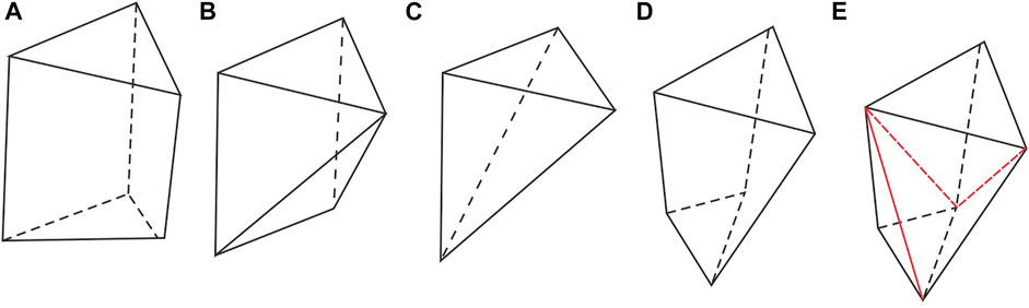
FIGURE 1. The geometric meaning of the GTP voxel: (A): A normal GTP, (B): Pyramid, (C): Degenerate to a tetrahedron, (D): Noncoplanar GTP, (E): The subdivision expression of the noncoplanar GTP, the red line is as the GTP subdivision split line.

There are also two degenerate forms of the GTP voxel, pyramid Figure 1B and tetrahedral voxel Figure 1C, which are usually used to build geological models with complex structures, such as the GTP on the border with faults and unconformable strata. The pyramid indicates that there is a borehole with zero length, and the tetrahedron indicates that the three boreholes intersect at a vertex. Most past studies have usually focused on the geometric solid model of geological entities (Zhu et al., 2012; Collon et al., 2020). In addition, the four points on the side of the GTP could be coplanar. Figure 1D illustrates a noncoplanar GTP, which will cause the calculation and analysis problem. The noncoplanar GTP should be divided into tetrahedrons or pyramids, as shown in Figure 1E.

The advantages of the GTP voxel model are as follows:

(1) The GTP is based on the design of geological borehole data features, and it can only use only the features of borehole data. The GTP edges are used to represent the borehole line, and the vertices represent the intersection of the borehole line and each stratum surface. The top and bottom triangles of the GTP model represent the different stratum surfaces.

(2) The GTP voxel model is not optimal for geological interpretation, which requires distinguishing the features between the bedding and the cross-bedding direction of the borehole strata, although it can easily explain the direction of the strata. As shown in Figure 1A, the borehole direction of the three GTP edges is also the cross-bedding direction, which represents the direction along a stratum and maintains the internal connection of the adjacent borehole.

(3) The model building and updating methods are simpler compared to the tetrahedron. The GTP model could be built by the Delaunay triangulation based on the coordinates of the top borehole orifice point (Pellerin et al., 2014), and then the TIN can be extended downward to obtain the GTP model. If there are new drilling exploration data, the model could only be updated by adding a new borehole using the TIN insertion method to update the model locally.

In addition, the disadvantage of the GTP model could be discussed as follows:

The GTP is an unstructured voxel, and the corresponding model refinement algorithm is difficult. The GTP model accuracy depends on the interval between adjacent boreholes. However, the horizontal spacing between boreholes is usually much larger than the vertical interval. Therefore, the accuracy is usually difficult to control and far from the requirements of 3D geological modeling. Studying how to improve the precision of GTP models can greatly extend their applicable scope, and the GTP interpolation method proposed in this paper is a novel solution.

Traditional GTP Geomodelling

In detail, the traditional GTP model building steps are as follows: First, the borehole, section data, survey data and stratigraphic data are obtained from the exploration data, the stratigraphic points of each borehole stratum are extracted separately to a pointset according to the geological structure, and then boundary constraints for special structures are added, such as faults and tunnels. Finally, these borehole points are projected to a suitable 2D plane (usually the XOY plane of the Cartesian coordinate system), and the fault and other discontinuous boundaries are added as constraint lines of the TIN. Then, the constraint Delaunay triangle building method is used to obtain the TIN surface. A GTP triangle extends downward along each borehole. All triangles are iterated, and all the GTP models are built. After iterating through all the boreholes and considering constraints, such as faults and stratigraphic boundaries, the GTP model is completed.

In addition, some rules should be followed in the GTP model building method (Che et al., 2015). First, the main rule is to ensure that the boreholes associated with a GTP voxel are in the same or adjacent GTP; second, the model accuracy is higher when the corresponding GTP voxel has better geometric features. At the same time, it is necessary to add supplemental data on the geological structure expression before building the GTP, which is used to ensure that the GTP automatic building algorithm can accurately rebuild the special geological structure, including faults and missing strata. The building steps of the specific GTP model considered in this work are as follows (De-fu et al., 2008). The workflow is shown as Figure 2.

(1) Multisource geological modeling data merging. The borehole data are merged with additional data, especially the section and topographic map data, which can be consistently cross-validated, as shown in Figure 3. At the same time, the section data are merged into the borehole data as the source data for building the GTP model.

(2) Complex geological structure preprocessing. For the combination of stratigraphic boundaries, simple faults and missing strata, a virtual borehole may be designed at the boundary of the fault plane and the missing stratum. It can be ensured that the correctness of the topological relationship of the GTP geometric model is acceptable, as shown in Figure 3. This is the basis for building the GTP model, and the specific design method can be found in many studies, but the GTP geometric optimization method has not yet been studied in-depth.

(3) Dividing the modeling area into many continuous interpolation units. According to the discontinuous boundary of a geological structure, the geological body needs to be divided into many continuous modeling units, and each unit is treated independently with different modeling parameters to reflect the natural world. These noncontinuous boundaries include ground surfaces, fault planes and artificially designated boundaries. The GTP model process cannot span two noncontinuous interpolation units.

(4) GTP voxel geometric model building and constrained Delaunay triangulation according to the borehole location. The GTP voxel model of each stratum is obtained by extending each triangle downward to the borehole bottom, three identical borehole strata are closed by adjacent GTPs, and the GTP connection methods used for multiple strata in the same borehole are always the same.

FIGURE 2

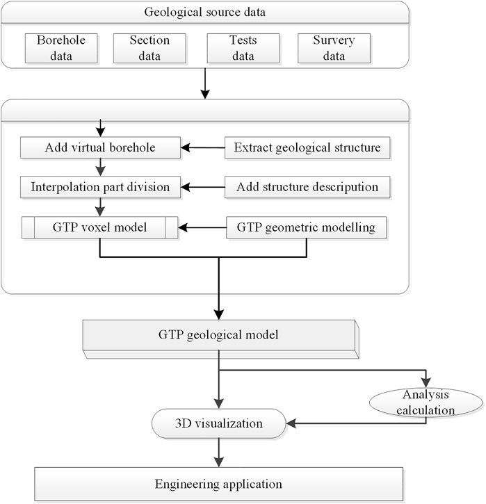
FIGURE 2. The classic GTP modeling workflow.

FIGURE 3

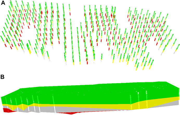
FIGURE 3. (A): The borehole distribution map, (B): The GTP model built based on the borehole data.

Nonsmooth Problem of the GTP Model

Much research on the building of GTP 3D geological models has been progressive, and great progress has also been made, but how to make GTP geological modeling methods more universal needs to be studied (Li et al., 2006). The accuracy of geological model building depends on the distribution density of borehole sampling. If borehole sampling is evenly and densely distributed, the change in model geometry is smooth, and the calculation accuracy is high. However, when the borehole sampling interval is large and the surface change is large, the GTP model changes drastically because the boreholes are connected by a straight line, and the stratum interface changes roughly. As shown in Figures 4A,B. When it is used for 3D visualization or spatial analysis, compared with the geological modeling method combined with geological interpolation, it reduces the application scenarios of sparse borehole sampling, and the practicality achieved is worth the reduction. The source data of the GTP voxel model is the entire borehole, but the existing interpolation methods are all based on discrete points. Thus, geostatistical interpolation methods cannot be directly applied.

FIGURE 4

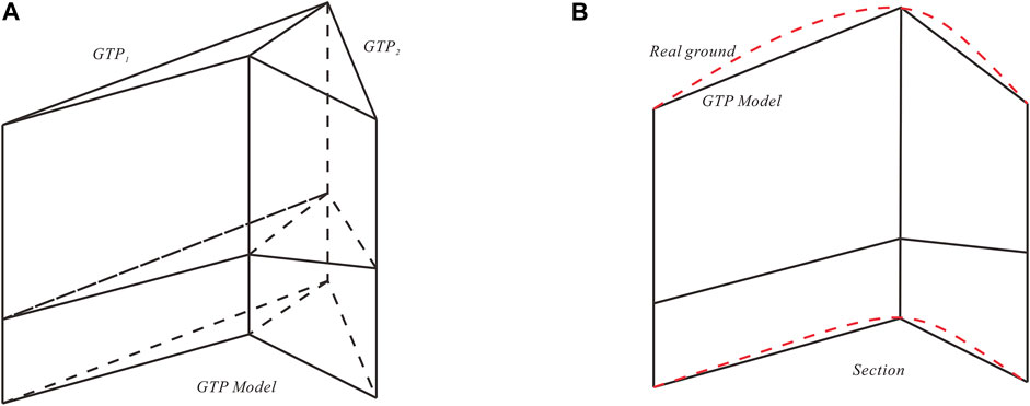
FIGURE 4. (A): The classic GTP model, (B): The real geological strata, the real ground is the red curve and the black segment is the GTP model.

The key points in solving the GTP nonsmooth problem are as follows:

(1) The classic GTP model of a rough area based on the borehole is inconsistent with the real situation. The classic GTP model is shown in Figure 4A, and the realistic ground of the same area in Figure 4B.

(2) The fusion problem between the GTP voxel model and the other interpolation method.

(3) Whether and where the model needs to be interpolated remains to be determined.

(4) Determining how to interpolate with high accuracy on the basis of the original GTP model needs to be addressed.

In the conventional GTP 3D model, the following nonsmooth problems exist:

(1) The top triangles of adjacent GTP voxels are too different, and the span between two adjacent GTPs is too long, resulting in sudden changes between a single GTP and the surroundings. Therefore, it does not meet the smoothness requirements.

(2) The smoothness between a single GTP is not uniform in the cross-bedding direction.

The stratigraphic smoothness between a single GTP and adjacent GTPs meets the requirements, but GTP modeling is meant to build a Delaunay triangle that passes through the orifice and extends downward, and the difference in the GTPs is not considered to be due to stratigraphic bedding. This building method cannot consider the smooth transition between adjacent GTPs in the cross-bedding and bedding directions, which means that the smoothness of different strata of the same GTP may be different and that there may be sub-GTPs in the strata; therefore, the smoothing condition is not satisfied, as shown in Figure 5.

(3) The distance between adjacent boreholes is too long, and the distribution of boreholes is uneven.

FIGURE 5

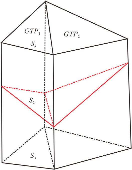
FIGURE 5. Two nonsmooth GTP in crossing-bed direction, and the red segments is the inner nonsmooth surface S₂.

A commonly encountered situation is when the distance between two adjacent boreholes is too long. The cross-bedding distance is much shorter than the bedding direction. At the same time, the boreholes are usually unevenly distributed and need interpolation.

The GTP Geometric Smoothness

Aiming at the geometric characteristics of the GTP, automatic refinement of the model was proposed in this paper. It is necessary to solve three main key problems. First, it is necessary to establish an accuracy standard to measure whether the current GTP model needs interpolation. Second, as is known, not all the model areas require interpolation; this is a local method and is faster than spatial interpolation, so the area should be calculated. Finally, the adaptive smoothness interpolation method should be studied to finish the process.

In this paper, an adaptive GTP interpolation method is proposed, and the key is to evaluate the areas where the model needs interpolation. To determine whether interpolation is required, several key factors need to be considered. First, whether the surface connection between each stratum changes smoothly when the boreholes are not dense enough; second, whether the building scheme can not only meet the 3D Delaunay rule but also satisfy the smooth transition of all strata at the same time and solve the discontinuity problem; third, whether the optimal building method can improve the GTP shape and accuracy. These issues are infrequently studied in research on the traditional GTP method, which also restricts the application of the GTP method.

The Definition of the GTP Smoothness

The method of building the GTP model directly based on borehole sampling data uses a GTP as the voxel to connect adjacent boreholes. Therefore, the two boreholes are connected in a straight line, and the stratigraphic plane fluctuates greatly. In the area with a large distance between the boreholes, the change between the two GTPs is not smooth, and the expression accuracy is not sufficient, meaning that it cannot reflect the real stratum change. The GTP smoothness can be defined as the change in the elevation of the GTP stratum surface relative to the surrounding area, and the calculation of the elevation smoothness of the GTP stratum surface is the key to realizing adaptive interpolation. For example, the angle calculated by two tangent derivatives of three consecutive points in the curve can be used to express the surface curvature and smoothness, and it can be used to evaluate the geometric changes of this curve, which can be seen as the smoothness. The rate of change is the degree of smoothness. Similarly, on a curved surface in the TIN, the change degree of two triangular surfaces can express the undulation, or the surface smoothness. Therefore, smoothing can be extended to the GTP interpolation evaluation through curve and surface expressions. For a 3D geological model, the smoothness and continuity of the surface is an important way to measure accuracy. Among the methods of discrete point interpolation, kriging interpolation uses a semivariogram to measure the weight that needs to be interpolated, and the spline function uses the derivative to calculate continuously. For 3D geological surfaces, the undulation rate of the surface can also be used to measure the model geometric fineness, but because the GTP model is based on boreholes, the top and bottom surfaces of the GTP model are related. The traditional method of building the GTP model is based on the top surface, which cannot simultaneously consider the accuracy of the top surface and the bottom surface; thus, this approach needs to be improved. This paper proposes a GTP interpolation method based on the smoothness of the top and bottom surfaces.

Specific evaluation factors for GTP smoothness include the following:

(1) The elevations of the top surface and bottom surface among the adjacent GTPs in each stratum change smoothly.

(2) The satisfaction degree with the 2D and 3D Delaunay rule of the GTP is evaluated. First, the satisfaction degree with the 2D Delaunay law of the triangle could be projected on the suitable plane on the top and bottom surfaces. Then, the 3D Delaunay rule of the tetrahedron is used to subdivide the GTP.

(3) The length difference between the borehole length and the height of the GTP is considered.

The calculation method of the GTP smoothness is introduced in this paper from the geometric curvature of the surface in computer geometric modeling. The Gaussian curvature of the surface used in the 3D computer aided design (CAD) software is employed as the main breakthrough point (Grafarend et al., 2014; Hayashi et al., 2021), and the Gaussian curvature is implemented at a certain point on the surface curvature, which refers to the product of the two principal curvatures at this point. The vertices on the surface are mapped to the center of the unit sphere, and the endpoint of the normal also should be mapped to the sphere, showing that a correlation is established between the points on the surface and the points on the certain sphere, which is called the spherical representation of the surface, or Gaussian mapping. The geometric meaning of Gaussian curvature is the limit of the area on the sphere or the local area of the surface, and it shows that the Gaussian curvature does reflect the local curvature of the surface. It is the main basis for analyzing the quality and smoothing of the surface. When the Gaussian curvature of the surface changes relatively quickly, the surface changes are relatively large, and the smoothness of the surface is low. The principal curvature represents an infinite number of orthogonal curvatures at a certain point on a curved surface, where there is a curve that makes the curvature extremely large, which is defined as the sum of the maximum curvature K_max. The curvature perpendicular to the maximal curvature surfaces is the minimum. In the minimum curvature K_min, K is expressed as the ratio of the second basic type and the first basic type of the surface, which is dependent on the point (u, v) of the surface z = r (u, v), as shown in Figure 6. The tangent direction function du/dv at this point is called the normal curvature K of the surface, it is along the tangent direction du/dv at this point, as shown in Figure 7. The Gaussian curvature reflects the degree of curvature of the current point and it is defined and calculated as Eqs 1, 2:

$K=\frac{LN-M^2}{EG-F^2}=\frac{1}{\left(EG-F^2\right)}\left[\left(r_u,r_v,r_{uu}\right)\left(r_u,r_v,r_{vv}\right)-{\left(r_u,r_v,r_{uv}\right)}^2\right]=K_{max}\text{∗}{K}_{min}(1)$

$K=\frac{1}{4\left(EG-F^2\right)}\left[E\left(E_v{G}_v-2F_u{G}_v+G_u^2\right)+F\left(E_u{G}_v-E_v{G}_u-2E_v{F}_v+4E_u{F}_v-2F_u{G}_u\right)+G\left(E_u{G}_u-2E_u{F}_v+E_v^2\right)-2\left(EG-F^2\right)\left(E_{vv}-2F_{uv}+G_{uu}\right)\right]\mathrm{and}E=r_u{r}_v,G=r_v{r}_v(2)$

FIGURE 6

FIGURE 6. A 3D point curvature on the triangular surface, the red arrows are the normals of the curve and the triangle.

FIGURE 7

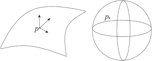
FIGURE 7. The surface curve expression in 3D space.

K is the partial differential of the surface. E, F, and G are the first invariants of the curved surface, while L, M, and N are the second invariants of the curved surface.

Using the positive and negative properties of Gaussian curvature, the structure of the surface adjacent to a point can easily be studied. The Gaussian curvature K > 0 is an ellipse point, K < 0 is a hyperbolic point, and K = 0 is a plane or parabolic point. Gaussian curvature is the intrinsic quantity of the surface; it is only related to the first basic type of the surface but is unrelated to the coordinate axes and the parameterized representation.

Therefore, in 3D CAD software, Gaussian curvature analysis is used to analyze the surface modeling. When the Gaussian curvature of the surface changes relatively quickly, it indicates that the internal change of the surface is relatively large, which means that the smoothness of the surface is lower. If the Gaussian curvatures of adjacent surfaces are considerably different across a shared boundary, then the surfaces are not continuous. This is usually called curvature discontinuity, indicating that the connection of the two surfaces is not smooth.

For the Gaussian curvature of a triangular surface, the calculation function is that $2\pi$ subtracts the sum of the angles ${\theta }_i$ of the point $N_i\left(v\right)$ corresponding to the neighborhood triangles, and then it can be divided by the corresponding surface area $A\left(v\right)$, the calculation method of the K(v)is shown as Eq. 3, for the scenario in Figure 8A:

$K\left(v\right)=\frac{1}{A\left(v\right)}\left(2\pi -{\displaystyle \sum _{v_{i\in N_i\left(v\right)}}{\theta }_i}\right)(3)$

FIGURE 8

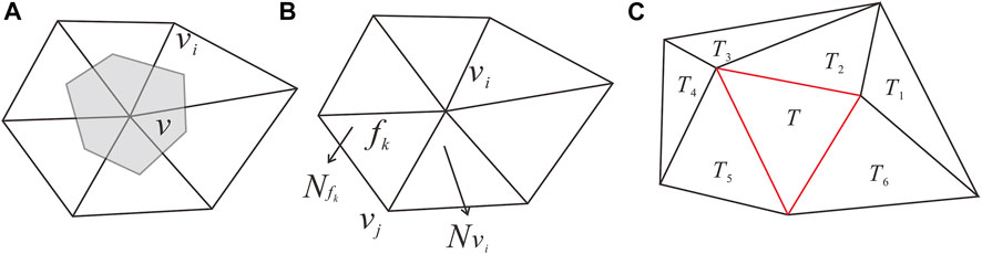
FIGURE 8. (A): The Gaussian curvature calculation of the triangular surface. (B) The GTP smoothness. (C) The GTP smoothness calculation method, where the red GTP is the currently considered GTP.

The Gaussian curvature can reflect the local undulation degree of the surface. The Gaussian curvature $N_{v_i}$ could be calculated using the Taubin method (Taubin, 1995) by the area of the weighted sum. Then, the smoothness $N_{top-GTP}$ of GTP can be defined from the top and bottom surfaces with Eq. 4:

$N_{top-GTP}=\max \left(N_{v_i},1\le i\le 3\right)(4)$

Whether a GTP is smooth and fine determines how it needs to be subdivided and interpolated, which depends on the top surface curvature N₁, the bottom surface curvature N₂, and the compliance with the 3D Delaunay rule, which is measured by G₃, and the weights of the corresponding GTPs are set as w₁, w₂, w₃. Then, the overall smoothness of a single GTP can be calculated using Eqs 5, 6:

$N_{GTP}=\frac{h_i}{{\displaystyle {\sum }_{1-n}h}}\left(N_{top}^i\cdot w_{top}^i+N_{bottom}^i\cdot w_{bottom}^i+G_3{w}_3\right)(5)$

$G_3=\frac{1}{max\left\{\left|\left(v_2-v_1\right)\right|,\left|\left(v_3-v_2\right)\right|,\left|\left(v_3-v_1\right)\right|\right\}}(6)$

where n is the number of strata, h is the vertical height of the current GTP, and i is the current stratum from all the iterated strata of this GTP (0 < i < n), as shown in Figure 8B.

GTP Model Smoothness Calculation

The interpolation method for the whole GTP model is as follows:

The interpolation calculation of a single GTP is mainly used to evaluate the smoothness and continuity between a GTP and adjacent GTPs, and whether it is required needs to be determined. For the smoothness calculation, the interpolation threshold needs to be set. When the threshold is met, the curvature calculation is automatically performed. Then, the adaptive interpolation calculation for the 3D geological model can be realized. The key to adaptive interpolation is the calculation method for the smoothness of each GTP. The process is divided into three steps. The weight value needs to be determined first, which is used as the GTP smoothness to determine whether the GTP needs to be interpolated, subdivided, and interpolation. Subdivision depends on the result of the GTP curvature defined in the last section. If it is greater than the calculation threshold, the subdivision will be performed; otherwise, the GTP will be maintained, as shown in Figure 8C:

(1) Gaussian curvature calculation iteratively occurs from the top surface and bottom surface of the GTP

The curvature calculation starts from the edge of the GTP model by iterating through all the GTPs according to their topological relationship. According to the definition of the curvature of the GTP, the Gaussian curvature of the top surface of the GTP can be calculated, which is recorded and stored in the GTP data object. The calculation method first iteratively calculates the curvature of the top and bottom surfaces of all GTPs. Then, the Gaussian curvature is considered, and the GTP curvature of each stratum of the sub-GTPs are calculated iteratively.

(2) Smoothness is calculated iteratively

All the GTP smoothness values could be calculated iteratively according to the definition of the GTP smoothness. According to the requirements of geological modeling accuracy, the interpolation classification threshold of each GTP should be preset, the different interpolation parameters are chosen for their suitability to different fineness levels, and the subdivision times and strategy of a GTP should be reasonably set to meet practical needs.

(3) Geological structure preprocessing

Before creating an accurate virtual borehole, it is necessary to preprocess the geological structural boundary. An uneven and discontinuous boundary of the geological structure cannot participate in interpolation and calculation because it needs to be marked in advance. These structures include sudden changes in the smoothness of the fault plane and the internal structure of an unconforming stratum, which need to be constrained and partitioned in advance. Smooth interpolation is performed within each partition, which cannot include different media. These special structures need to be calculated separately; they include both sides of the fault, the inner edge of the missing stratum, and the internal structures, such as pinch offs and lenses.

Virtual Borehole Design for Interpolation

Methodology

In the previous section, the calculation method of GTP smoothness is studied. According to the threshold and the fineness requirements control of the model, the area that needs to be interpolated can be determined through iterative calculation. The GTP model refinement method based on fineness control is also seen as the model interpolation method. The interpolation method first needs to comply with the existing GTP data structure; boreholes are used as the main data source to build the model, and then the model interpolation can be completed. This method is usually adopted when there is no actual drilling data available from existing research. A virtual borehole is added to the constrained boundary of the GTP model. The virtual and actual boreholes have the same geological media, and the stratigraphic elevation of the virtual borehole can be calculated by the actual borehole, which can ensure that the stratum properties (and assignment logic) are similar to those of the surrounding boreholes. The constraint conditions, such as uneven changes in a stratum due to faults and folds, are considered to ensure that the transition between virtual boreholes and real boreholes is natural, and this is consistent with the actual geological structure. Therefore, this article also chooses the virtual borehole method to solve the smoothing problem and fulfill the accuracy requirement. This is mainly realized by inserting virtual boreholes in key positions. The specific process includes the following steps:

(1) Whether a virtual borehole needs to be inserted could be determined.

(2) The insertion method of the virtual borehole position should be designed, following the GTP subdivision method.

(3) The stratigraphic point elevation in each virtual borehole could be calculated.

The design of the virtual borehole position plays a vital role in the interpolation process. First, for the current GTP, the adjacent GTPs index can be calculated iteratively. Then, the internal topological relationship of the GTPs can be used to quickly find the shared edges, shared faces and adjacent edges, as well as the faces between the GTPs, for fast calculation.

The design method and workflow are as follows:

(1) The calculation precision w is set.

According to the smoothness of the overall 3D geological model, a determination of whether each GTP requires interpolation is made.

(2) The virtual borehole position could be determined according to the subdivision number and calculation method.

According to the predetermined smoothness, if the GTP needs to be interpolated, the appropriate calculation method of the new borehole position should be determined, which means that different smoothnesses need different calculation methods. The number of virtual boreholes will be discussed in Section 4.2 (GTP subdivision method), and the borehole calculation method will be discussed in detail in Section 4.3 (Virtual borehole calculation method). Then, the new borehole position is calculated if interpolation is necessary. The direction of the inserted borehole is usually parallel to the boreholes of the current GTP model.

(3) The stratigraphic elevation calculation of the inserted virtual borehole should be performed.

The virtual borehole calculation is mainly aimed at the elevation calculation of the intersection point between the borehole and the stratum surface, as discussed in Section 4.3 (Virtual borehole calculation method), and the equal division method is mainly used.

(4) The special geological structure boundary is preprocessed.

For special geological structures, such as faults and folds, it is necessary to follow the basic GTP processing method that the virtual boreholes may be inserted on the boundary location to complete the special structure processing (Maxelon et al., 2009; Royse, 2010).

GTP Subdivision Method

According to the smoothness calculated in the previous section, the usual method for one or several surrounding GTPs requires multiple subdivisions to achieve smoothing and refinement of the GTP model. The top and bottom of the GTP are realized, and the number of specific subdivisions is related to the deviation of the threshold. Moreover, the subdivision method and the corresponding smoothness are closely related to the interpolation method. Assuming that the threshold of N_GTP is set to N, the number of corresponding subdivided GTPs is n, and the obtained precision is c. As each precision choice is different to determine for the best method, a comparison table of accuracy and selected method can be developed. The parameters could be preset according to the detailed model and interpolation accuracy requirement. The relationship between the accuracy, smoothness, subdivided GTPs and the subdivision methods are shown in Table 1:

TABLE 1

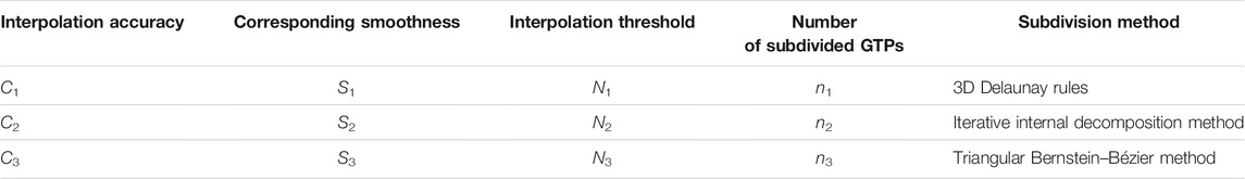
TABLE 1. The relationship between the accuracy, smoothness, number of subdivided GTPs and the subdivision method.

The iterative internal decomposition method is suitable for a case of high smoothness. When the smoothness does not meet the threshold requirement, the difference is not much larger at the same time, and the current GTP can be directly split once or twice to obtain the result. The center point of the decomposition (virtual borehole position) selection and calculation is the key factor. The shape of the existing GTP should be considered. If the error is not sufficiently great, the point could be inserted at the gravity center of the triangle, so that the same GTP will be broken into three sub-GTPs. The surface can be smoother on the top and bottom surfaces. The advantage of this internal decomposition method is that smooth interpolation can be achieved without changing the existing built GTP model. Triangle subdivision can be performed with different methods.

To meet the interpolation requirements, multiple subdivisions are performed by inserting virtual boreholes in the internal GTP or sub-GTPs based on the iterative internal decomposition method, as shown in Figure 12. However, in extreme cases, the subsequent interpolation process may produce GTPs of poor quality, which usually include long and narrow triangles; in this situation, GTP model optimization and rebuilding are needed.

If the smoothness requirement is still not met after one subdivision, multiple subdivisions are needed. The subdivision method should be run adoptedly with multiple virtual borehole insertions; therefore, the method of inserting the borehole should be refer to the building method of the uniformly subdivided triangle. The position calculation methods of the quadratic and cubic subdivisions are discussed in Sections 4.2, 4.3.

According to the requirements of the 3D Delaunay rule, the minimum difference between the internal angle and the optimal angle is where the tetrahedral subdivision of the GTP is performed. In several schemes of inserting new boreholes, the conformity of the 3D Delaunay rule for each quadrilateral is determined, and finally, the best plan is chosen by comparing different solutions.

Virtual Borehole Calculation Method

The calculation method of virtual boreholes mainly considers the top position. In the previous section, the methods for obtaining the number and position of the inserted virtual borehole are discussed, but each stratigraphic elevation value also needs to be calculated. A new stratigraphic elevation calculation of the virtual borehole is proposed by implementing the Bernstein-Bézier quadratic triangle (BBQT) method (Li, 2011; Weber et al., 2011). This method is similar to the triangulate extension from the spline curve to spline surface, this method is suitable with the local surface interpolation without other data, so the calculation speed is faster than the spatial interpolation method, and the accuracy is stable. In particular, there is no need to change the existing model, and all the interpolation points are on the triangulate surface. The N- degree triangle has number of (n+1) (n+2)/2 control points of v_{1,2 … ,n}, the three sides of the triangle should be divided into n equal parts. The BBQT triangle could be built by connecting the control points as Figure 9, the TIN could be built through iterating all triangles. This is called the control grid or Bézier grid. Then, according to the Bernstein-Bézier polynomial theory, the n degree Bernstein polynomials $B_{i,j,k}^n$ are linearly independent and they form a complete n-degree polynomial, as shown in Eq. 7. Thus, it is also called the Bernstein basis functions a P_n, and this could meet the unit decomposition requirements, the ${\lambda }_1,{\lambda }_2,{\lambda }_3$ are the volume coordinate of any point, and i, j, and k are the iterative sequence numbers of the three vertices:

$B_{i,j,k}^n\left({\lambda }_1,{\lambda }_2,{\lambda }_3\right)=\frac{n!}{i!j!k!}{\lambda }_1^i{\lambda }_2^j{\lambda }_3^k,i+j+k=n,{\displaystyle \sum _{i+j+k=n}{B}_{i,j,k}^n}=={\left({\lambda }_1+{\lambda }_2+{\lambda }_3\right)}^n=1(7)$

FIGURE 9

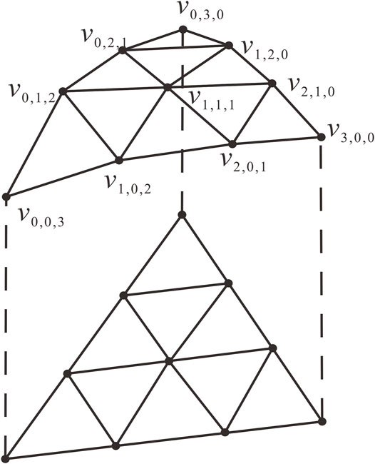
FIGURE 9. The BBQT division method, the control points and the control grid.

The row vector composed of all Bernstein polynomials of degree n is denoted as Eqs 8,9:

$B^1=\left[\begin{array}{ccc}{B}_{\mathrm{1,0,0}}^1& B_{\mathrm{0,1,0}}^1& B_{\mathrm{0,0,1}}^1\end{array}\right]=\left[\begin{array}{ccc}{\lambda }_1& {\lambda }_2& {\lambda }_3\end{array}\right](8)$

$B^2=\left[B_{\mathrm{2,0,0}}^2{B}_{\mathrm{1,1,0}}^2{B}_{\mathrm{1,0,1}}^2{B}_{\mathrm{0,2,0}}^2{B}_{\mathrm{0,1,1}}^2{B}_{\mathrm{0,0,2}}^2\right]=\left[{\lambda }_1^{2}2{\lambda }_1{\lambda }_{2}2{\lambda }_1{\lambda }_3{\lambda }_2^{2}2{\lambda }_2{\lambda }_3{\lambda }_3^2\right](9)$

Then, it could be converted to the Cartesian coordinate system, because any n variable quadratic polynomial, as Eq. 10:

$f\left(x,y\right)={\displaystyle \sum _{i+j\le n}{a}_{i,j}{x}^i{y}^j}=f\left({\lambda }_1,{\lambda }_2,{\lambda }_3\right)={\displaystyle \sum _{i+j+k=n}{b}_{i,j,k}{B}_{i,j,k}^n\left({\lambda }_1,{\lambda }_2,{\lambda }_3\right)}=B^n{f}_b(10)$

The geometric meaning of the BBQT division method is shown in Figure 9. As in the above method, the stratigraphic point of each virtual borehole could be obtained, and all the virtual boreholes could be calculated iteratively through this method.

Adaptive GTP Smoothness Interpolation Geomodeling Methodology

For the GTP voxel, the top and bottom surfaces are both triangles. Each stratigraphic surface is a TIN surface composed of the top and bottom surfaces of the GTP. The degree of undulation and the thickness of the strata are also collectively determined by the top and bottom surfaces. Each triangle in the TIN is adjacent to several triangles, the Gaussian curvature of the three vertices of the triangle on the top surface of each GTP is calculated correspondingly, and the maximum Gaussian curvature value should be selected as the GTP smoothness, which could measure the undulation and determine whether interpolation is required, as shown in Figure 10. The mainly key factor of the adaptive smoothness interpolation is as following:

FIGURE 10

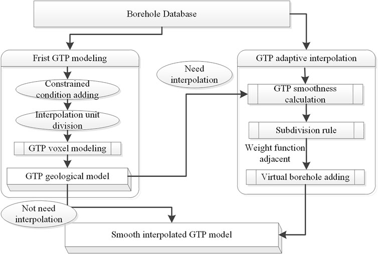
FIGURE 10. The GTP model interpolation flow and adaptive GTP smoothness interpolation geomodelling methodology.

The traditional GTP building method needs to consider constraint conditions. The constraints refer to faults, caves, boundaries, etc., and the relevant GTPs must be marked to provide a control parameter for iterative interpolation. The GTP that needs interpolation cannot cross the constraint boundary; that is, its smoothness cannot be calculated with the surrounding GTPs outside the boundary. Then, the GTP model is finished by building the interpolation unit iteratively.

Then, the smoothness of each GTP is calculated, the GTPs that do not meet the smoothness standard are recorded, and the GTP subdivision method and virtual borehole interpolation calculation are performed. After one subdivision, the smoothness of the current GTP should be recalculated to determine whether it needs to be subdivided. This iteration will stop when the smoothness threshold set by the interpolation is met, and the adaptive interpolation of the model will be completed at that time.

Adaptive GTP Smoothness Interpolation Geomodelling

The adaptive interpolation method of the GTP model is the focus of this work. It is different from the traditional uniform geometric subdivision method. This research method focuses on the inclusion of adaptive interpolation for the GTP voxel geological model, and this process provides the same accuracy with a small amount of data. The key to this process is to obtain the GTP smoothness, which is a criterion for adding a virtual borehole. If the smoothness is greater than the given setting value, an appropriate number of virtual boreholes can be inserted; otherwise, it will not be performed, and the process is iterated until the entire interpolation process is completed. The following is a step by step description, as shown in Figure 10:

(1) GTP geological model building

As discussed in the second section, the GTP geometric model was built based on the original boreholes. The method is designed to determine all of the boreholes with the same number of strata, then Delaunay triangulation based on the top surface points is performed, and the TIN should be extended downward to obtain the GTP model of all strata. For complex geological models, there are usually many unconformities, including lenses, missing strata, and faults. It is also necessary to retain the GTP of the missing stratum.

(2) GTP smoothness calculation

According to the smoothness research scheme proposed in previous studies, the smoothness of a GTP can be calculated. The smoothness of the three vertices of the top surface of the GTP could be used to obtain the smoothness of a single GTP, and then GTPs of other strata could be built by the same three boreholes following the order from top to bottom. The GTP smoothness should be calculated and stored.

(3) Adaptive GTP division by adding a virtual borehole

First, the preset threshold to end interpolation is determined. This value is set to a reasonable value according to the accuracy requirements of the model, the amount of data, and the calculation time. The smoothness needs to be obtained based on multiple experiments. Whether the preset threshold is exceeded can then be determined; if it is greater than the threshold, a new virtual borehole inside the current GTP can be added. There are two solutions that can be attempted for the virtual borehole location. The preferred position is the center or gravity center of the GTP. In the second attempt, multiple boreholes are added, referring to the triangular Bernstein-Bézier subdivision method. Virtual boreholes can be inserted at the subdivision node position using the existing spline surface to obtain the elevation value.

(4) Iterative interpolation process

The smoothness of the interpolated initial GTP is recalculated. If it is still greater than the threshold, steps 2) and 3) should be repeated until the requirements are met, and the interpolation process of the entire geological model is completed. Finally, a highly accurate 3D geological model can be obtained.

GTP Model Optimization Rebuilding

After the last section, a smooth and fine GTP voxel model can be obtained, or the newly added borehole may generate some deformed GTPs, which need to be optimized and rebuilt. In addition, the GTP interpolation method used is the virtual borehole insertion method added to the center, and thus, there is no smoothing process for the boundary of the unconformity stratum, and optimization and reconstruction are also needed. The specific research plans for the two cases are as follows:

(1) Deformed GTP optimization method

According to the assignment of virtual borehole stratum, the value assignment method is based on the stratigraphic point of each stratum, but the GTP voxel is a volume model, and the stratum is a solid unit. The upper and lower strata are separated from the assignment method, which may cause a deformative GTP. The rebuilding method checks the topological relationship of each voxel. If there is a topological error, for example, it is known that the bottom elevation of the GTP in the same stratum is higher than the top surface. Therefore, it is necessary to study optimization methods, such as the geometric subdivision method in geometry and the reconstruction method.

(2) Boundary GTP rebuilding method

The boundary rebuilding of the GTP model of the missing strata is necessary. During the interpolation process in the last section, the unconformity boundary is still the same as before the interpolation, the accuracy is not high enough, and the discontinuity changes suddenly. Thus, the GTP on the boundary optimization is needed, and new borehole points are added in the middle to ensure that the stratigraphic boundary is smooth and a closed polyline. The rebuilding method could insert virtual boreholes to the boundary, the virtual borehole number and position could be calculated using the spline curve method (Notaroˇ, 2013), this is shown as Figure 11.

FIGURE 11

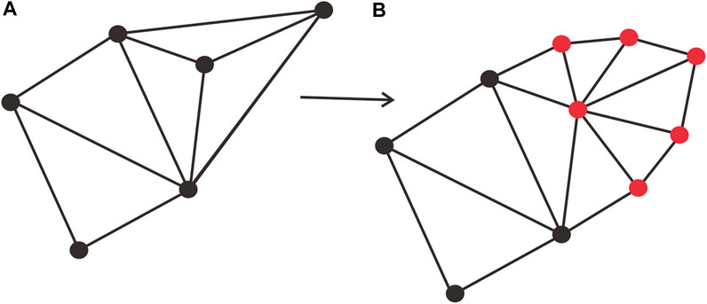
FIGURE 11. The boundary optimization method. (A): The original model on the boundary of the missing strata, (B): The new model on the boundary after interpolation with virtual borehole (red color point).

Application and Example

We attempt to verify the feasibility and accuracy of the adaptive GTP interpolation method proposed in this paper. The research area is geological exploration data from Dalian, Liaoning Province, China. The 3D geological model could provide auxiliary decision-making and mining analysis for economic geology, urban construction, and underground engineering design, so the proposed method is of great significance to the economic geological analysis of the study area. In this case, the geological structure and economic value of minerals in the study area is the most concerned, it is necessary to build a 3D geological model to understand the spatial distribution of various elements in the subsurface, this could provide many supports to the economic geology through spatial analysis and calculation. To simplify the problem, only part of the areas data is selected, and there are a total of 41 boreholes, as shown in Figure 12A. 6 strata were detected, 488 GTPs were built according to the boreholes through traditional GTP modeling method, as shown in Figure 12B. Based on the GTP adaptive interpolation framework and process mentioned in the article, the traditional GTP model was built first. The initial GTP is understood according to the drilling exploration data, the section data, and the regional knowledge, 138 virtual boreholes were designed as shown in Figure 13A. The GTP geometric modeling method is used to build a GTP stratigraphic model, with a total of 586 independent GTPs, as shown in Figure 13B. This also describes all the stratigraphic and geometric constraints in as much detail as possible. There are unsmoothed regions in the model, including the unsmoothed between two GTPs and the different strata of the same GTP that cannot meet the smoothness requirements, and the smooth interpolation of the GTP needs to be considered.

FIGURE 12

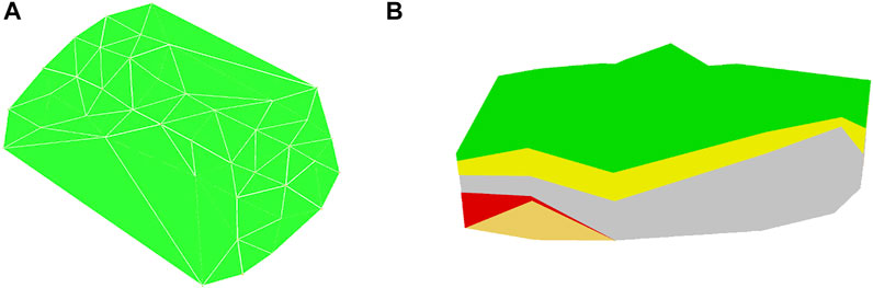
FIGURE 12. (A): The triangular surface built by using the data from the original 41 borehole, (B): The GTP model built from the classic method.

FIGURE 13

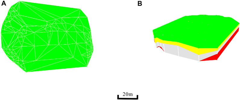
FIGURE 13. (A): The 138 virtual boreholes by the adaptive GTP interpolation method, (B): The adaptive GTP interpolation method based on 41 borehole data.

First, the interpolation smoothness parameter is preset. The calculated smoothness results suggest that 12 GTPs need to be interpolated twice and that 5 GTPs need to be interpolated multiple times. Among them, 32 GTPs are used in the center point decomposition method, and 13 GTPs are used in the subtriangular decomposition method. After multiple interpolations, the model smoothness meets the requirements. Compared with the previous interpolation, the smoothness is improved, and the adjacent GTPs and the boreholes are excessively smooth. At the same time, the geometric shapes of the GTPs are better, which proves that the Delaunay triangle rule is satisfied.

In addition, the accuracy of the adaptive interpolation can be proven by cross-validation. A total of 200 borehole sample points are excluded to validate the interpolation value using the proposed method. The horizontal axis is the interpolation value, the vertical axis is the sample value, the trendline is y = x, and the cross-validation result is shown in Figure 14.

FIGURE 14

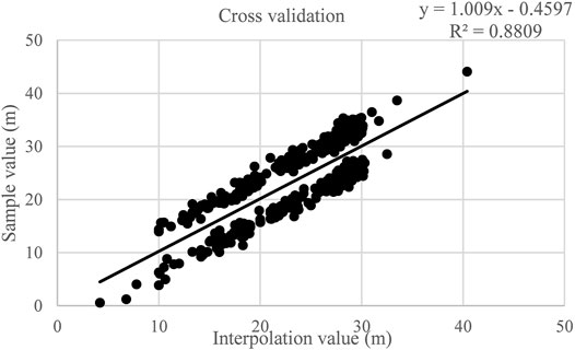
FIGURE 14. The cross validation results.

Conclusion

As known for its simplicity and high efficiency, the GTP geological model designed for the borehole data structure is usually widely used, and the GTP model accuracy usually determines the borehole sample density. However, in the traditional GTP modeling method, the adjacent borehole distance is much greater than the stratigraphic thickness, and the GTP model is not sufficient for precise analysis. Thus, GTP interpolation approaches for improving model accuracy must be studied urgently, as the lack of an appropriate approach limits the widespread application of the GTP modeling method.

To solve these problems, first, the GTP geometric smoothness standard was proposed to measure the GTP model accuracy, which is used to evaluate whether and where the GTP voxel model needs interpolation; second, adaptive GTP subdivision using the virtual borehole method was discussed in depth under the condition of GTP smoothness control and was used to obtain a high-accuracy GTP model without changing the existing GTP geometric voxel data structure. In summary, the GTP model adaptive interpolation framework based on GTP smoothness was established in this paper, and high-quality results were achieved through engineering application case verification.

In future work, the virtual borehole calculation method during the GTP interpolation process could be improved; as a result, fewer parameter settings would allow the user to finish the interpolation by automation, which could be an important point of GTP model interpolation in the future.

Data Availability Statement

The original contributions presented in the study are included in the article/Supplementary Material, further inquiries can be directed to the corresponding author.

Author Contributions

Conceptualization, LS; methodology, YW, HC, and LS; software, LS and JX; validation, JY and SW; writing—review and editing, LS.

Funding

This research was funded by the “National Key Research and Development Program of China, Grant Number 2018YFC1508602” and “National Natural Science Foundation of China, grant number U19A2049.”

Conflict of Interest

The authors declare that the research was conducted in the absence of any commercial or financial relationships that could be construed as a potential conflict of interest.

Publisher’s Note

All claims expressed in this article are solely those of the authors and do not necessarily represent those of their affiliated organizations, or those of the publisher, the editors and the reviewers. Any product that may be evaluated in this article, or claim that may be made by its manufacturer, is not guaranteed or endorsed by the publisher.

Acknowledgments

The authors would like to thank the editor and reviewers, the “National Natural Science Foundation of China” and the “Ministry of Science and Technology of China” for the funding support.

References

Abdul-Rahman, A., and Pilouk, M. (2008). Spatial Data Modelling for 3D GIS. Springer. doi:10.1007/978-3-540-74167-1

CrossRef Full Text | Google Scholar

Bai, T., and Tahmasebi, P. (2020). Hybrid Geological Modeling: Combining Machine Learning and Multiple-Point Statistics. Comput. Geosci.. doi:10.1016/j.cageo.2020.104663

CrossRef Full Text | Google Scholar

Bickel, P., Diggle, P., Fienberg, S., Wermuth, N., and Zeger, S. Interpolation of Spatial Data: Some Theory for Kriging.

Caumon, G., Lévy, B., Castanié, L., and Paul, J.-C. (2005). Visualization of Grids Conforming to Geological Structures: A Topological Approach. Comput. Geosciences 31, 671–680. doi:10.1016/j.cageo.2005.01.020

CrossRef Full Text | Google Scholar

Charifo, G., Almeida, J. A., and Ferreira, A. (2013). Managing Borehole Samples of Unequal Lengths to Construct a High-Resolution Mining Model of mineral Grades Zoned by Geological Units. J. Geochemical Exploration 132, 209–223. doi:10.1016/j.gexplo.2013.07.006

CrossRef Full Text | Google Scholar

Che, D.-f., Jia, G.-b., and Jia, Q.-r. (2015). Key Technology of 3D Geosciences Modeling in Coal Mine Engineering. J. Shanghai Jiaotong Univ. (Sci.) 20, 21–25. doi:10.1007/s12204-015-1582-2

CrossRef Full Text | Google Scholar

Che, D., and Jia, Q. (2019). Three-Dimensional Geological Modeling of Coal Seams Using Weighted Kriging Method and Multi-Source Data. IEEE Access 7, 118037–118045. doi:10.1109/access.2019.2936811

CrossRef Full Text | Google Scholar

Che, D., Wu, L., and Xu, L. (2006). “Study on 3D Modeling Method of Faults Based on GTP Volume,” in Proceeding of the 2006 IEEE International Symposium on Geoscience and Remote Sensing, Denver, CO, USA, Aug. 2006 (IEEE). doi:10.1109/IGARSS.2006.411

CrossRef Full Text | Google Scholar

Collon, P., Rongier, G., Parquer, M., Clausolles, N., and Caumon, G. (2020). “Uncertainty Assessment in Subsurface Modeling: Considering Geobody Shape and Connectivity in Complex Systems,” in EGU General Assembly Conference Abstracts, 5641.

Google Scholar

Cui, Y., Li, Q., Li, Q., Zhu, J., Wang, C., Ding, K., et al. (2017). A Triangular Prism Spatial Interpolation Method for Mapping Geological Property Fields. Int. J. Geo-Information 6, 241. doi:10.3390/ijgi6080241

CrossRef Full Text | Google Scholar

Čuma, M., Wilson, G. A., and Zhdanov, M. S. (2012). Large-scale 3D Inversion of Potential Field Data. Geophys. Prospecting 60, 1186–1199. doi:10.1111/j.1365-2478.2011.01052.x

CrossRef Full Text | Google Scholar

D’Affonseca, F. M., Finkel, M., and Cirpka, O. A. (2020). Combining Implicit Geological Modeling, Field Surveys, and Hydrogeological Modeling to Describe Groundwater Flow in a Karst Aquifer. Hydrogeol. J. 28, 2779–2802. doi:10.1007/s10040-020-02220-z

CrossRef Full Text | Google Scholar

De-fu, C., Li-xin, W., and Zuo-ru, Y. (2008). On the GTP-Based 3D Modeling Method for Complex Geological Body. Int. Geosci. Remote Sens. Symp. 2, 3–5. doi:10.1109/IGARSS.2008.4779243

CrossRef Full Text | Google Scholar

Fan, W., Wang, B., Paul, J.-C., and Sun, J. (2013). An Octree-Based Proxy for Collision Detection in Large-Scale Particle Systems. Sci. China Inf. Sci. 56, 1–10. doi:10.1007/s11432-012-4616-5

CrossRef Full Text | Google Scholar

Feizi, F., Karbalaei-Ramezanali, A. A., and Farhadi, S. (2021). Application of Multivariate Regression on Magnetic Data to Determine Further Drilling Site for Iron Exploration. Open Geosci. 13, 138–147. doi:10.1515/geo-2020-0165

CrossRef Full Text | Google Scholar

Forster, B., and Massopust, P. (2011). Multivariate Interpolation with Fundamental Splines of Fractional Order. Proc. Appl. Math. Mech. 11, 857–858. doi:10.1002/pamm.201110416

CrossRef Full Text | Google Scholar

Ghaleshahi, Z. G., Karbalaeiramezanali, A., Eyvazkhani, S., and Kashefi, K. K. (2015). Interpretation of Magnetic Data in Biaj Area of Hamedan. Iran.

Google Scholar

Glynn, P. D., Jacobsen, L., Phelps, G., Bawden, G., Grauch, V., Orndorff, R., et al. (2011). 3D/4D Modeling, Visualization and Information Frameworks: Current US Geological Survey Practice and Needs. Geol. Surv. Canada, Open File 6998, 33–38. Three-Dimensional Geol. Mapping; Work. Ext. Abstr. Minneapolis, Minnesota. doi:10.4095/289609

CrossRef Full Text | Google Scholar

Grafarend, E. W., You, R.-J., and Syffus, R. (2014). Map Projections. doi:10.1007/978-3-642-36494-5

CrossRef Full Text | Google Scholar

Hayashi, K., Jikumaru, Y., Ohsaki, M., Kagaya, T., and Yokosuka, Y. (2021). Discrete Gaussian Curvature Flow for Piecewise Constant Gaussian Curvature Surface. Computer-Aided Des. 134, 102992. doi:10.1016/j.cad.2021.102992

CrossRef Full Text | Google Scholar

Hillier, M., Wellmann, F., Brodaric, B., Kemp, E. De., and Schetselaar, E. (2021). Three-Dimensional Structural Geological Modeling Using Graph Neural Networks. Math. Geosci. 53 (8), 1725–1749. doi:10.1007/s11004-021-09945-x

CrossRef Full Text | Google Scholar

Hodkiewicz, P. (2014). “The Future of Geological Modelling,” in Unearthing 3D Implicit Model., 26–31.

Google Scholar

Hua, J., He, Y., and Qin, H. (2004). “Multiresolution Heterogeneous Solid Modeling and Visualization Using Trivariate Simplex Splines,” in Proc. Ninth ACM Symp. Solid Model. Appl., 47–58.

Google Scholar

Jacquemyn, C., Jackson, M. D., and Hampson, G. J. (2018). Surface-Based Geological Reservoir Modelling Using Grid-free NURBS Curves and Surfaces. Math. Geosci. 51, 1–28. doi:10.1007/s11004-018-9764-8

CrossRef Full Text | Google Scholar

Li, F. J. (2011). Interpolation and Convergence of Bernstein-Bézier Coefficients. Acta Math. Sin.-English Ser. 27, 1769–1782. doi:10.1007/s10114-011-8462-y

CrossRef Full Text | Google Scholar

Li, Q., Chen, X., Zhang, H., Gao, J., Zhang, W., and Shi, C. (2006). A 3D Integral Data Model for Subsurface Entities Based on Extended GTP. Int. Geosci. Remote Sens. Symp., 1519–1522. doi:10.1109/IGARSS.2006.392

CrossRef Full Text | Google Scholar

Li, C.-J., Chen, J., and Chen, W.-J. (2011). A 3D Hexahedral Spline Element. Comput. Structures 89, 2303–2308. doi:10.1016/j.compstruc.2011.08.005

CrossRef Full Text | Google Scholar

Liu, H., Chen, S., He, L., Hou, M., and Zhang, J. (2020). Generalized Triangular Prism Interpolation Method for Geotechnical Parameter Characterization. Bull. Eng. Geol. Environ. 79, 3417–3435. doi:10.1007/s10064-020-01772-4

CrossRef Full Text | Google Scholar

Lixin, W., and Wenzhong, S. (2004). GTP-based Integral real-3D Spatial Model for Engineering Excavation GIS. Geo-spatial Inf. Sci. 7, 123–128. doi:10.1007/BF02826649

CrossRef Full Text | Google Scholar

Lu, G. Y., and Wong, D. W. (2008). An Adaptive Inverse-Distance Weighting Spatial Interpolation Technique. Comput. Geosciences 34, 1044–1055. doi:10.1016/j.cageo.2007.07.010

CrossRef Full Text | Google Scholar

Mansouri, E., Feizi, F., and Karbalaei, R. (2015). Identification of Magnetic Anomalies Based on Ground Magnetic Data Analysis Using Multifractal Modelling: a Case Study in Qoja-Kandi, East Azerbaijan Province, Iran. Nonlinear Process. Geophys. 22, 579–587. doi:10.5194/npg-22-579-2015

CrossRef Full Text | Google Scholar

Maxelon, M., Renard, P., Courrioux, G., Brändli, M., and Mancktelow, N. (2009). A Workflow to Facilitate Three-Dimensional Geometrical Modelling of Complex Poly-Deformed Geological Units. Comput. Geosciences 35, 644–658. doi:10.1016/j.cageo.2008.06.005

CrossRef Full Text | Google Scholar

Mei, G., Xu, N., and Xu, L. (2016). Improving GPU-Accelerated Adaptive IDW Interpolation Algorithm Using Fast kNN Search. Springerplus 5, 1389. doi:10.1186/s40064-016-3035-2

PubMed Abstract | CrossRef Full Text | Google Scholar

Notaroˇ, B. M. (2013). B-spline Entire-Domain Higher Order Finite Elements for 3-D Electromagnetic Modeling. IEEE Microwave Wireless Components Lett. 22, 497–499. doi:10.1109/lmwc.2012.2217123

CrossRef Full Text | Google Scholar

Oliveira, S., Johnson, C. A., Juliani, C., Monteiro, L., Leach, D. L., and Caran, M. (2021). Geology and Genesis of the Shalipayco Evaporite-Related Mississippi Valley-type Zn–Pb deposit, Central Peru: 3D Geological Modeling and C–O–S–Sr Isotope Constraints. Miner. Depos. 56, 1–20. doi:10.1007/s00126-020-01029-w

CrossRef Full Text | Google Scholar

Pellerin, J., Lévy, B., and Caumon, G. (2014). Toward Mixed-Element Meshing Based on Restricted Voronoi Diagrams. Proced. Eng. 82, 279–290. doi:10.1016/j.proeng.2014.10.390

CrossRef Full Text | Google Scholar

Ran, J. A., Yl, A., Gw, A., Ejc, B., Yc, A., Chao, W. C., et al. (2021). A Stacking Methodology of Machine Learning for 3D Geological Modeling with Geological-Geophysical Datasets, Laochang Sn Camp, Gejiu (China) - ScienceDirect. Comput. Geosci. 151, 104754. doi:10.1016/j.cageo.2021.104754

CrossRef Full Text | Google Scholar

Rongier, G., Collon, P., and Renard, P. (2017). A Geostatistical Approach to the Simulation of Stacked Channels. Mar. Pet. Geology. 82, 318–335. doi:10.1016/j.marpetgeo.2017.01.027

CrossRef Full Text | Google Scholar

Royer, J. J., Mejia, P., Caumon, G., and Collon, P. (2015). 3D and 4D Geomodelling Applied to Mineral Resources Exploration-An Introduction. Miner. Resour. Rev., 73–89. doi:10.1007/978-3-319-17428-0_4

CrossRef Full Text | Google Scholar

Royse, K. R. (2010). Combining Numerical and Cognitive 3D Modelling Approaches in Order to Determine the Structure of the Chalk in the London Basin. Comput. Geosciences 36, 500–511. doi:10.1016/j.cageo.2009.10.001

CrossRef Full Text | Google Scholar

Schmitt, B., Kazakov, M., Pasko, A., and Savchenko, V. (2000). Volume Sculpting with 4D Spline Volumes,” in CISST’2000, International Conference on Imaging•@Science, Systems, and Technology 2, 475–483. Available from: http://citeseerx.ist.psu.edu/viewdoc/download?doi=10.1.1.97.7810&rep=rep1&type=pdf.

Google Scholar

Stein, M. L. (1999). Interpolation of Spatial Data: Some Theory for Kriging. Springer Series in Statistics, 41–43. doi:10.1080/00401706.2000.10485731

CrossRef Full Text | Google Scholar

Taubin, G. (1995). “Curve and Surface Smoothing without Shrinkage,” in Proceedings of IEEE international conference on computer vision (IEEE), Cambridge, MA, USA, June 1995 (IEEE), 852–857.

Google Scholar

Wang, Z., Zuo, J., Yuan, C., and Xie, H. (2015). A Source Data-Driven Method for 3D Geological Modeling in Coal Mines. Int. J. SAFE 5, 113–123. doi:10.2495/SAFE-V5-N2-113-123

CrossRef Full Text | Google Scholar

Wang, W., Sun, L., Li, Q., and Jin, L. (2017). Representing the Geological Body Heterogeneous Property Field Using the Quadratic Generalized Tri-prism Volume Function Model (QGTPVF). Arab. J. Geosci. 10, 115. doi:10.1007/s12517-017-2930-3

CrossRef Full Text | Google Scholar

Watson, C., Richardson, J., Wood, B., Jackson, C., and Hughes, A. (2015). Improving Geological and Process Model Integration through TIN to 3D Grid Conversion. Comput. Geosciences 82, 45–54. doi:10.1016/j.cageo.2015.05.010

CrossRef Full Text | Google Scholar

Weber, D., Kalbe, T., Stork, A., Fellner, D., and Goesele, M. (2011). Interactive Deformable Models with Quadratic Bases in Bernstein-bézier-form. Vis. Comput. 27, 473–483. doi:10.1007/s00371-011-0579-6

CrossRef Full Text | Google Scholar

Wu, L. (2004). Topological Relations Embodied in a Generalized Tri-prism (GTP) Model for a 3D Geoscience Modeling System. Comput. Geosciences 30, 405–418. doi:10.1016/j.cageo.2003.06.005

CrossRef Full Text | Google Scholar

Zhu, L.-F. (2008). Construction Method and Actualizing Techniques of 3D Visual Model for Geological Faults. J. Softw. 19, 2004–2017. doi:10.3724/SP.J.1001.2008.02004

CrossRef Full Text | Google Scholar

Zehner, B., Börner, J. H., Görz, I., and Spitzer, K. (2015). Workflows for Generating Tetrahedral Meshes for Finite Element Simulations on Complex Geological Structures. Comput. Geosciences 79, 105–117. doi:10.1016/j.cageo.2015.02.009

CrossRef Full Text | Google Scholar

Zhu, L., Zhang, C., Li, M., Pan, X., and Sun, J. (2012). Building 3D Solid Models of Sedimentary Stratigraphic Systems from Borehole Data: An Automatic Method and Case Studies. Eng. Geology. 127, 1–13. doi:10.1016/j.enggeo.2011.12.001

CrossRef Full Text | Google Scholar