Simulation of Glacial Lake Outburst Flood in Southeastern Qinghai-Tibet Plateau—A Case Study of JiwenCo Glacial Lake

Glacial lake outburst floods (GLOFs) is one of the main natural disasters in alpine areas, which can cause extreme destruction to downstream settlements and infrastructures. A moraine-dammed lake named JiwenCo glacial lake (JGL) in the southeastern Qinghai-Tibetan Plateau failed on 26 June 2020, destroying many buildings, roads, bridges, and farmlands along the flow path. We reconstructed the process of this GLOF event by the Hydrological Engineering Center’s River Analysis System (HEC-RAS) and examined the JGL’s evolution (area, length, and volume) before its outburst, based on the measured cross sections and hydrological data, videos, and pictures taken by inhabitants, DEM data, and Landsat Thematic Mapper (TM)/Enhanced Thematic Mapper (ETM+)/Operational Land Imager (OLI) images. The result showed that area, length, and volume of the JGL increased by 0.20 ± 0.07 km², 0.66 ± 0.03 km, and 0.03 ± 0.001 km³ from 1988 to 2020 (before the outburst), respectively. Approximately 0.05 km³ of water volume was discharged with the dropped water level of 15.63 m after the outburst. The peak flow was 534.4 m³/s at breach and increased to 1,408.11 m³/s at Zhongyu town. The difference between the simulated and measured peak flows in Zhongyu town was 41.88 m³/s (3.53%), showing the high accuracy of the modeling results. For villages along the river-channel, the highest velocity was found in Yiga village (14.23 m/s) and the lowest was in Gongwa village (1.22 m/s). The maximum depth was gradually increased as the river reached downstream, 8.03 m in Yiga village and 50.96 m in Duiba village. The combination of landslide, high temperature, and extremely heavy precipitation resulted in this GLOF disaster. An integrated disaster prevention and mitigation plan needs to be developed for susceptible areas such as Niduzangbo basin that experienced two GLOFs in recent 10 years.

1 Introduction

The Qinghai-Tibetan Plateau has the largest amount of snow and ice around the world, except for the North and South Pole (Yao Tandong et al., 2012). Against the background of intense climate warming (IPCC, 2021), the accelerated retreat of glaciers and the dramatic increase in meltwater have led to the massive formation and rapid expansion of glacial lakes (Nie et al., 2018; Ma et al., 2021). A series of glacier-related disasters, such as glacial lake outburst floods (GLOFs) and debris flow, have also been caused (Chen et al., 2015; López-Moreno et al., 2016; Yao et al., 2019). China’s Tibet Autonomous region is a high incidence area of GLOFs, which witnessed 27 glacial lake outbursts since 1960 (Yao et al., 2014; Jia and Cui, 2020). These GLOFs caused severe damages to infrastructures and people’s lives and property in downstream areas. For example, the outburst flood from the CirenmaCo glacial lake in 1984 destroyed the China-Nepal Friendship Bridge and buildings at the Zhangmu port in Nyalam county, and damaged part of the Sunkosi hydropower plant in Nepal. Meanwhile, 200 people were killed in this incident (Yao et al., 2014). The outburst flood from the Decoga glacial lake, which is located at the Shannan region of Tibet Autonomous region, washed away 18 bridges and killed two people on 18 September 2002 (Tong et al., 2019). The RanzeriaCo glacial lake broken up on 5 July 2013, which outburst flood washed away 49 buildings and caused the economic loss of 0.27 billion CNY (Sun et al., 2014).

Moraine-dammed glacial lakes, formed between the moraines abandoned on the glacier foreland and the glacier snout, are most subject to outburst relative to other glacial lakes such as supraglacial lake, glacial erosion lake (Lv and Li, 1986; Liu et al., 1988; Xu and Feng, 1989). Moraine dam is usually made of loose material with low cohesion and contains ice-cores inside. It is unstable and unconsolidated because ice-cores under moraine are prone to melt affected by warming and thermokarst (Richardson and Reynolds, 2000; Qin, 2014). Undoubtedly, reviewing historical GLOFs events contributes to improve our understanding on trigger mechanisms and magnitude of glacial lake outburst, and helps to develop disaster contingency measurement plans for future GLOFs (Nie et al., 2020). A detailed case study on historical GLOFs can not only provide more information about the whole GLOFs process including causes of failure and subsequent impact, but also improve the accuracy of hazard evaluation (Nie et al., 2018). Therefore, this study focuses on the JiwenCo glacial lake (JGL) outburst flood recently occurred in southeastern Qinghai-Tibetan Plateau and aims to 1) quantify the evolution of JGL before the outburst; 2) simulate the peak flow and its travel-time at breach and downstream villages after the dam broke; 3) reconstruct the depth, velocity, and inundated extent of this flood at selected downstream villages.

2 Study Area

The JGL (93°37′48″E, 30°21′36″N) located at the southwestern Niduzangbo basin was formed by retreat of glacier with a GLIMS_ID of G093642E30319N (Figure 1). The area and water-level of this lake were 0.57 km² and 4,465 m in 2020, respectively. The JGL is only 5.1 km away from Yiga village, with a height difference of 640 m. It burst on 26 June 2020, destroying many farmlands and vital infrastructures including roads, bridges, and houses. Its area and water-level became 0.26 km² and 4,450 m after the outburst. The scenic spot named Yiga under construction, which received an investment of 8.4 million CNY, was completely flooded. As a subbasin of the Yigongzangbo basin, the Niduzangbo basin is located in the southeast of the Qinghai-Tibetan Plateau with an altitude range of 3,183–6,901 m. This basin is in the subhumid monsoon climate zone of the plateau, characterized by cold winters and cool summers, the coexistence of heat and rain with the heaviest precipitation in June and July (Sun et al., 2014; Duan et al., 2020). There are numerous glaciers developed in this basin (Figure 1B), which are marine-glacier and are experiencing dramatic ablation due to the ongoing warming (Shangguan et al., 2008; Nie et al., 2012; Xiang et al., 2013).

FIGURE 1

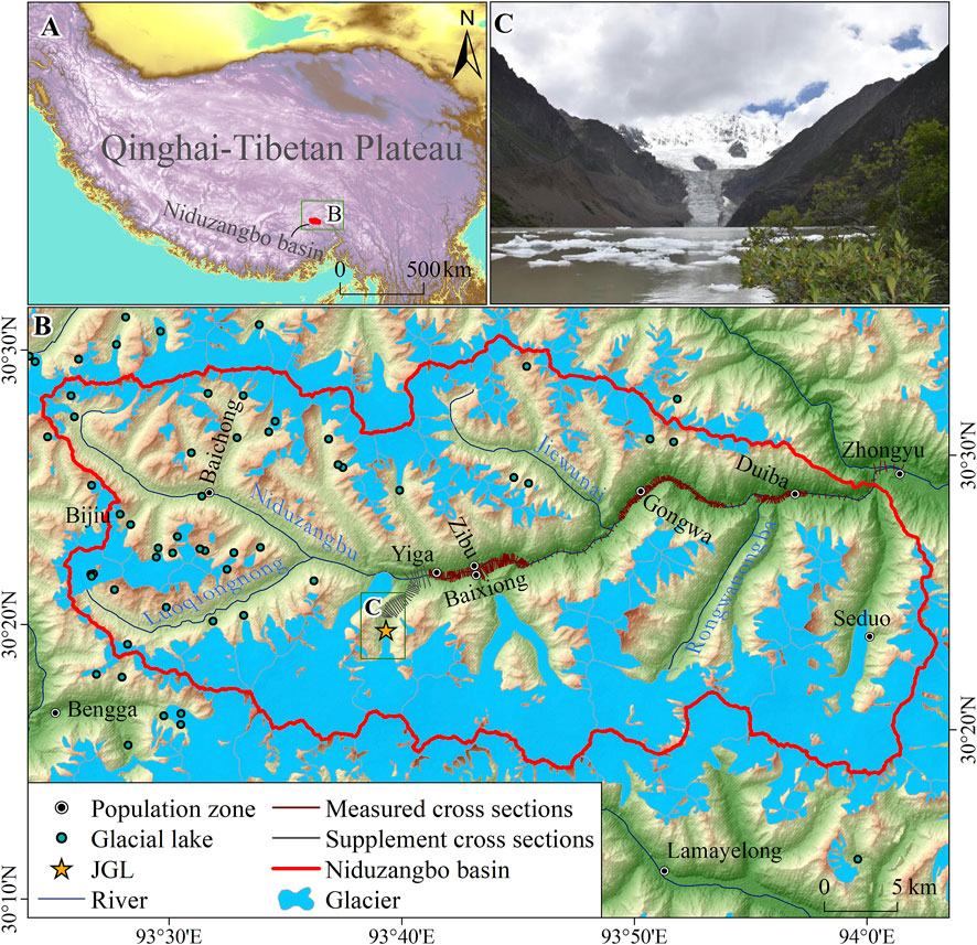
FIGURE 1. Location of the study area. (A) is the location of the Niduzangbo basin in the Qinghai-Tibetan Plateau. (B) is the geographical setting of the Niduzangbo basin and locations of measured and supplement cross sections. (C) is the photo of JGL taken by Yao in 2017.

3 Materials and Methods

3.1 Materials

3.1.1 Satellite Image

Satellite image is widely used to delineate the past and present glacial lakes, which is also highly feasible to detect historical GLOFs events (Sattar et al., 2019; Veh et al., 2019; Nie et al., 2020). In this study, we adopted the optical images including Landsat Thematic Mapper (TM)/Enhanced Thematic Mapper (ETM+)/Operational Land Imager (OLI) image and GF1_WFV4 image to map the failed JGL and its mother glacier, and qualify their evolution within the past 3 decades. Niduzangbo basin is part of the pathway transported warm and moist flow northward from the Indian Ocean, so it is covered by perennial clouds. A total of 19 scenes of Landsat TM/ETM+/OLI image (Orbit: 136039) and one scene of GF1_WFV4 (E93.7N30.9) image were selected based on the criterion of little cloud cover on the JGL (Table 1). They were acquired from the website of the United States Geological Survey (USGS, https://earthexplorer.usgs.gov/) and the Chinese High-resolution Earth Observation System (CHEOS, https://www.cheosgrid.org.cn/), respectively. Meanwhile, we selected a scene of Sentinel-2A Multi-Spectral Instrument (MSI) image to validate the accuracy of JGL boundary from the Landsat image due to its higher spatial resolution. This Sentinel-2A image (Tile: T46REU) was downloaded from the website of European Space Agency (ESA, https://scihub.copernicus.eu/).

TABLE 1

TABLE 1. The information of the images used in this study.

3.1.2 Measured Cross Sections and Terrain Data

We measured the Niduzangbo river-channel on 3 May 2020. From Zhongyu town to Yiga village along the Niduzangbo, there were 260 cross sections being measured with a total measured distance of 40.61 km (Figure 1B). The Advanced Land Observing Satellite-1 (ALOS) DEM was selected to combine with measured cross sections to produce a new terrain data, which was a very crucial parameter for performing 2D dam-break simulation. The ALOS DEM were acquired from the website of NASA’s EARTHDATA (https://earthdata.nasa.gov/) with a spatial resolution of 12.5 m.

3.1.3 Land Use and Land Cover

The dam-break flood was propagated over a large spatial extent where the surface roughness varies considerably. Therefore, we need to set different Manning’s n values for different areas to indicate the varying roughness over the propagation extent to obtain a more accurate reconstruction. The measured cross sections recorded the land cover on both sides of the river channel, including forest, artificial surface, grassland, cultivated land, shrub, and bareland. The global land cover dataset obtained from this website (http://data.ess.tsinghua.edu.cn/) was adopted to determine the land cover for 28 supplemental cross sections (Figure 1B), which has a spatial resolution of 10 m. The Manning’s n value for different land cover was determined by referring to the HEC-RAS (River Analysis System): Users’ Manual (Brunner. 2010) (Table 2).

TABLE 2

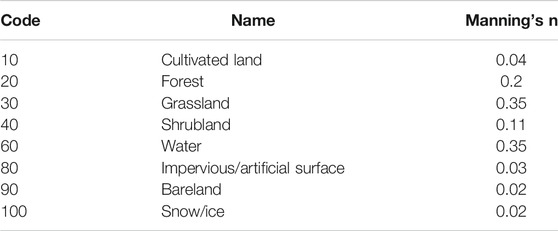
TABLE 2. Code, name, Manning’s n of different land cover used in this study (Brunner, 2010).

3.1.4 Field Investigation Information

In July 2017, we carried out a field investigation on JGL and got its information such as the width of outlet, the status of surrounding glacier and terrain. After its outburst, we went to Zhongyu town to investigate the disaster on August 20–25 2020. The residents of Zhongyu town are mainly engaged in agricultural and animal husbandry. The transportation infrastructure in this town is underdeveloped and most roads run parallel with rivers because of the restricted terrain (Figure 2A). We held an interview with some inhabitants living in the villages downstream of JGL on 25 August 2020 (Figures 2B,C), some of them witnessed the process of JGL’s outburst and downstream propagation. This interview was conducted in their cropland and was recorded by cellphone. Next to the cropland was the road damaged by the flood, which was completely impassable and was being rebuilt when we were interviewing (Figure 2D). From the interview and materials including videos and photos before and after the outburst provided by the inhabitants, we learned that the JGL began to break at 7:30 a.m. and reached its peak flow at 10:00 a.m., which was very useful for simulating this GLOFs event and determining its cause. Moreover, the measured hydrological data at the Zhongyu Hydrological Station were also obtained during field visit.

FIGURE 2

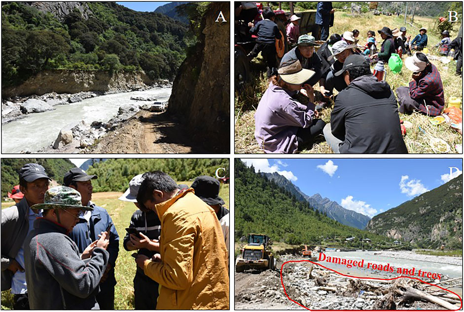
FIGURE 2. (A) The road beside the river between the Zhongyu town and the JGL. (B) On-site interview with residents. (C) Researchers were watching videos of the outburst provided by residents. (D) The scene after being washed away by the flood.

3.2 Methods

3.2.1 Lake Delineation

Lake mapping is a prerequisite for quantifying the evolution of glacial lakes and performing GLOFs simulations. Normalize Difference Water Index (NDWI) proposed by McFeeters (1996) is the most common method for automated water mapping because it can distinguish between snow/ice and water body; meanwhile, most sensors have two bands involved in the NDWI equation, i.e., green and near-infrared (termed as NIR hereinafter) (Li and Sheng, 2012). It takes advantage of the fact that the water has strongly contrasting reflectance in the green band and the NIR band, and the difference in reflectance between the water and other features can be enhanced by the ratio (Frey et al., 2010; Bhardwaj et al., 2015). We chose the Landsat OLI image acquired on 19 August 2016 with fewer clouds to map the JGL boundary automatically. Figure 3 illustrates the total procedure of lake delineation. We first calibrated the raw digital numbers (DNs) of each pixel to the Top-Of-Atmosphere (TOA) reflectance. Then the calculation equation of NDWI (Eq. 1) was adopted to automatically detect the extent of JGL. The optimal binary image of the JGL and its background features was obtained by setting the threshold interactively and then was converted into a vectorized polygon; this study chose 0.16 as the optimal threshold. Finally, we got the optimal outline of the JGL by manual revision.

$\mathit{NDWI}=\frac{{\mathit{\rho }}_{\mathit{Green}}-{\mathit{\rho }}_{\mathit{NIR}}}{{\mathit{\rho }}_{\mathit{Green}}+{\mathit{\rho }}_{\mathit{NIR}}}(1)$

where ρ_Green and ρ_NIR are the TOA reflectance in the green band and the NIR band, respectively.

FIGURE 3

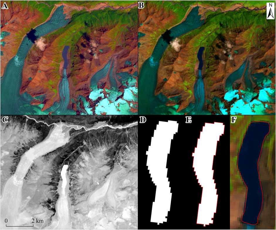
FIGURE 3. Process of automated lake delineation. (A) is Landsat OLI composed image (acquired on 18 August 2016, band 6-5-2 as RGB); (B) is image after performing radiometric calibration and flash atmospheric correction; (C) is NDWI image; (D) is the extent of the JGL when the threshold is 0.16; (E) is the JGL outline in a vector format overlapped on the binary image; (F) is the JGL outline after manual revision.

We overlaid the JGL boundary in 2016 derived from the above procedure on the other images (in total 19 scenes of image) to delineate lake boundaries for the corresponding years. The same as the above procedure was adopted to map JGL’s mother glacier, but only 5 years’ boundaries (1988, 2003, 2010, 2016, and 2020) were extracted because of the intensive effect of cloud cover.

3.2.2 Volume Estimation

As a basic parameter of lake, volume has an important role in the hazard assessment of glacial lakes and simulation of GLOFs. Most studies used empirical equations to calculate it due to the absence of bathymetric data. These empirical equations were proposed for certain regions, taking volume as a function of lake area. For example, Huggel et al. (2002) proposed an empirical equation for the Swiss Alps, which was widely used in glacial lakes researches (Jain et al., 2012; Sattar et al., 2020). Loriaux and Casassa (2013) proposed an empirical equation for the Northern Patagonia Icefield. In this study, the equation proposed by Zhou et al. (2020) was adopted to calculate the JGL’s volume. Zhou et al. (2020) proved that this equation is suitable for calculating volume of moraine-dammed lake in different regions. The equation is as follows:

$\mathit{V}=0.0717{\mathit{w}}^2\mathit{l}(2)$

It uses the width (w) and length (L) of each moraine-dammed lake to calculate the volume from the perspective of three-dimensional morphological characteristics, where V, w, and l is the volume, width, and length of the JGL, respectively.

3.2.3 Accuracy Validation and Error Elevation

In this study, the method for verifying the accuracy of lake outline derived from the above procedure was to compare it with the visually interpreted lake outline based on the Sentinel-2A MSI image with a higher spatial-resolution. There is a high consistency between the two results (Figure 4). The JGL’s area was 0.04 km² smaller than that result from visual interpretation, which accounts for 7.1% of the lake area by visual interpretation. This is understandable given that the time span between the two data sources was 4 months, during which JGL was expanding. Therefore, the JGL’s outline in this study had a high accuracy and the 0.16 was the optimal threshold for mapping JGL from the Landsat image acquired on 19 August 2016.

FIGURE 4

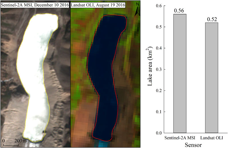
FIGURE 4. The comparison between lake outline obtained by our method and that obtained by visual interpretation reference to Sentinel-2A MSI image.

The error in the lake outline derived from image interpretation is mainly attributed to image resolution and co-registration (Hall et al., 2003; Yao Xiaojun et al., 2012). The images adopted did not involve registration between different sensors, so only the error caused by the image resolution was considered in this study, which can be calculated by Equation 3 proposed by Wang et al. (2012).

$\mathit{\epsilon }=\frac{{\mathit{\lambda }}^2\cdot \mathit{p}}{2\sqrt{{\mathit{\lambda }}^2+{\mathit{\lambda }}^2}}=\frac{\mathit{\lambda }\cdot \mathit{p}}{2\sqrt{2}}(3)$

where ε is the area error, λ is the image resolution (Landsat TM image being 30 m and Landsat ETM+/OLI image being 15 m), and p is the perimeter of the lake.

The length accuracy is affected by the accuracy of lake outline and the quality of DEM data; however, Yao et al. (2015) demonstrated the effect from the latter is negligible. 50% of the boundary pixels were included in the interpretation process, so the JGL length error is the spatial resolution of image, i.e., 30 m for Landsat TM image, 15 m for Landsat ETM+/OLI image.

The equation of volume error is as follows based on the law of error propagation

$\mathit{\mu }=0.0717\sqrt{{\left(2\mathit{wl}\right)}^2{\mathit{\sigma }}_{\mathit{w}}^{\mathrm{2}}+{\left({\mathit{w}}^2\right)}^2{\mathit{\sigma }}_{\mathit{l}}^{\mathrm{2}}}(4)$

where μ is the volume error, б_l is the length error, and б_w is the width error.

3.2.3 GLOF Simulation

The Hydrological Engineering Center’s River Analysis System (HEC-RAS) is a professional software to carry out hydrological analysis, which was widely adopted in glacial hazard researches (Anacona et al., 2015; Satter et al., 2019; Nie et al., 2020; Sattar et al., 2021). It provides us with a platform to perform one-dimensional (1D) steady/unsteady and two-dimensional (2D) unsteady flow river hydraulics calculations (Brunner, 2010). In this study, we performed 1D unsteady flow simulation employing HEC-RAS V5.0.3 to obtain flow curve at the breach of JGL during outburst. Geometric data is one of the necessary parameters, which consists of the river-channel and cross section (Brunner, 2010). First, we mapped a flow path (river-channel) based on the Google Earth image. Then, the cross-sections table was converted and input into HEC-RAS software. Finally, the reach length, the demarcation points, and Manning’s n value of the river-channel and river-bank were filled in based on the measured record-table. A total of 288 cross sections were entered, including 260 measured cross sections and 28 supplemental cross sections. These supplemental cross sections were produced in ArcGIS based on ALOS DEM, which satisfied the following conditions: 1) perpendicular to the river channel; 2) the distance between two adjacent cross sections being within 100–500 m, and encryption being performed for areas with sharp changes in height; 3) the length of the cross section covering the whole floodplain. The cross-section numbers were listed in a descending order, which were required by HEC-RAS software. The boundary condition is another key parameter of the HEC-RAS 1D model. We used the stage hydrograph as an upstream boundary condition, which was obtained according to the lake-level before and after the outburst and the time span between the initiation of the failure and the appearance of peak flow (Brunner, 2010). The measured flow hydrograph from the Zhongyu Hydrological Station was set as the downstream boundary condition. Two later inflows, 1 m³/s and 898 m³/s, were added to the 260th and second cross sections, respectively. The former represented the inflow from the upstream of Niduzangbo River and the latter represented the flow between the confluence of JGL’s outflow and Niduzangbo River and the confluence of Niduzangbo River and Yigongzangbo River; they were provided by Zhongyu Hydrologic Station.

HEC-RAS V5.0.7 was adopted to perform 2D unsteady flow simulation to reconstruct the flood propagation in the downstream area and its damage for the villages, because the 2D model can produce spatially distributed flow properties such as water-depth and velocity (Chanson, 2004; Brunner, 2010). It applies an implicit finite volume algorithm to solve the full 2D Saint Venant equations or 2D Diffusion Wave equations (Brunner, 2010). Several studies demonstrated that the 2D hydraulic model had better performance than the 1D model in obtaining the inundated extent (Horritt and Bates, 2002; Anacona et al., 2015). We delineated the positions of JGL and moraine-dam, and a 2D flow area containing the JGL and Zhongyu town in the Google Earth image. Then, the parameters of moraine-dam were input, which include the width of breach and the dam elevation pre- and post-outburst, etc (Table 3). We produced a mesh with a spatial resolution of 12.5 m for this 2D flow area, and each cell of this mesh was assigned a different elevation and Manning’s n value based on terrain and land cover. The hydrographs at the outlet derived from the 1D model were selected as an upstream boundary condition of 2D unsteady flow simulation. The downstream boundary condition was consistent with the 1D model.

TABLE 3

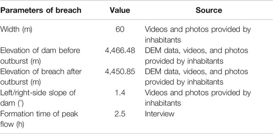
TABLE 3. Parameters of moraine-dam.

4 Results

4.1 JGL and Its Mother Glacier Evolution in 1988–2020

JGL has undergone a dramatic expansion toward its mother glacier in the past 30 years (Figure 5); this evolution pattern is similar to the most moraine-dammed glacial lakes in this basin, such as the RanzeriaCo glacial lake (Sun et al., 2014). The area, length, and volume of JGL increased by 0.20 ± 0.07 km², 0.66 ± 0.03 km, and 0.03 ± 0.005 km³ from 1988 to 2020 (before the outburst), respectively, from 0.37 ± 0.05 km² to 0.57 ± 0.04 km², 1.26 ± 0.03 km to 1.92 ± 0.02 km, and 0.03 ± 0.003 km³ to 0.06 ± 0.003 km³. We observed accelerated growth for JGL during the study period: 0.003 ± 0.03 km²/a (1988–2001), 0.006 ± 0.05 km²/a (2001–2010), and 0.01 ± 0.05 km²/a (2010–2020) for area; 0.01 ± 0.003 km/a (1988–2001), 0.02 ± 0.003 km/a (2001–2010), and 0.04 ± 0.002 km/a (2010–2020) for length; 0.0004 km³/a (1988–2001), 0.0003 km³/a (2001–2010), and 0.002 km³/a (2010–2020) for volume. After the outburst, the JGL’s area, length, and volume decreased to 0.26 ± 0.03 km², 1.50 ± 0.02 km, and 0.01 ± 0.001 km³, respectively, which were 54, 21.9, and 81.2% less than that on 24 June 2020.

FIGURE 5

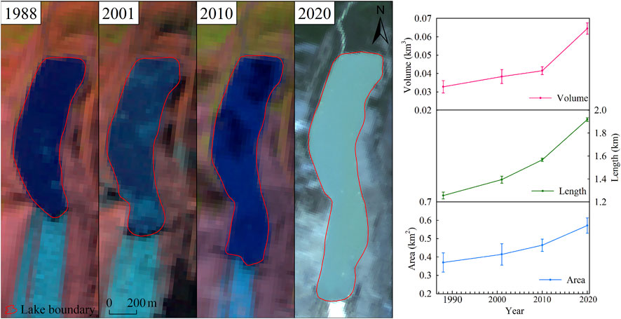
FIGURE 5. Changes in the area, length, and volume of the JGL in 1988–2020. Backgrounds are the Landsat TM image (Bands 5, 4, 3) acquired on 9 October 1988 and 30 November 2001, Landsat ETM + image (Bands 5, 4, 3) acquired on 28 September 2010, and GF1_WFV4 image acquired on 24 June 2020 respectively.

Only five scenes of image with minimal cloud cover and free snow were used for the delineation of JGL’s mother glacier. As shown in Figure 6, JGL’s mother glacier was in retreat over 1988–2020. Its area was 11.23 km² in 1988 and reduced to 9.81 km² in 2020 with the total recession and rate of −1.42 km² and −0.44 km²/a, respectively.

FIGURE 6

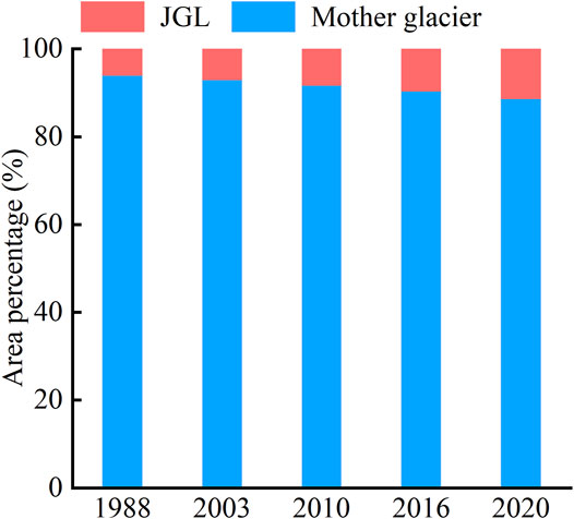
FIGURE 6. The proportionality between JGL and ablation area of its mother glacier at different times.

4.2 GLOF From the JGL

Water volume of approximately 0.05 km³ was discharged based on the parameters set for moraine-breach. We obtained the flow curves at breach, Zibu village, Baixiong village, Gongwa village, Duiba village, and Zhongyu town located downstream of JGL (Table 4). The breach was completely formed within 7.50 h (Figure 7), the peak flow at the outlet was 534.40 m³/s and appeared at 2.50 h after the outburst. Zibu and Baixiong villages are located 9.50 km downstream of the lake, and the peak flow arrived at 2.72 h after the burst. The peak flow (528.20 m³/s) was similar to that at the breach, because the grits, soil, and vegetation in the channel between the breach and these two villages attenuated the flow, but the high cliff between them intensified the flow momentum. The peak flow in the Gongwa village located at 23.67 km downstream of the JGL appeared at 3.25 h after the moraine-dam failure, and the peak flow (516.23 m³/s) was lower than the breach (18.17 m³/s). The peak flow in the Duiba village located at 36 km downstream of the breached lake appeared at 3.64 h after the dam-break, and the peak flow (512.35 m³/s) was lower than the breach (22.05 m³/s). The peak flow in the Zhongyu town was 1,408.11 m³/s, which occurred at 3.86 h after the breach; this result differs from the measured peak flow (1,360 m³/s) obtained at Zhongyu Hydrological Station by 48.11 m³/s. The difference between the measured and simulated peak flows is only 3.53% of the measured peak flow, indicating the high accuracy of this simulation. Therefore, this proved the feasibility of taking the flow curves at the breach we obtained as upper boundary conditions for 2D dam-breach simulations and the suitability of using HEC-RAS to simulate GLOFs on the southeastern Qinghai-Tibetan Plateau.

TABLE 4

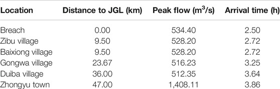
TABLE 4. Peak flow and arrival time at different villages.

FIGURE 7

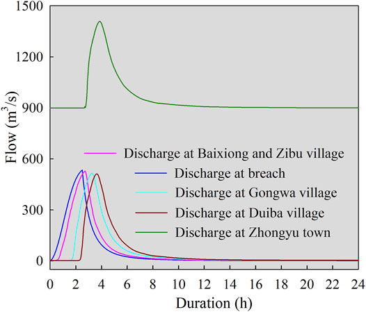
FIGURE 7. The discharge hydrograph at different locations along flow channel.

Our simulation showed the water level of JGL decreased by 15.63 m after the outburst. Figure 8, 9 illustrate the spatial distribution of hydraulic properties (depth and velocity). Most buildings in the Yiga village were submerged (Figures 8A, 9A) when the flood passed with the maximum depth of 8.03 m and the maximum velocity of 14.23 m/s. The distance and height difference between the Zibu village and the Niduzangbu river-channel were approximately 240.74 and 16.8 m, respectively; therefore, only several houses in the east of Zibu village were inundated with the maximum depth of 1.94 m and the maximum velocity of 1.22 m/s (Figures 8B, 9B). However, the Baixiong village was completely submerged when the flood arrived since it was only 68.96 m from the river-channel with the similar altitude as the river (Figures 8C, 9C). The maximum depth and the velocity in the Baixiong village were 16.25 m and 4.74 m/s, respectively. The road and bridge connecting these two villages were damaged by flooding with the maximum depth and velocity of 22.62 m and 15.26 m/s, respectively. The Gongwa village is located on the west side of the river-channel and has very few houses (Figures 8D, 9D). This village was partially submerged when the flood passed, the maximum depth was 21.9 m, and the maximum velocity was 9.66 m/s. The Duiba village is located at a plain area on the east side of the river, distributed along both sides of the road (Figures 8E, 9E). When the flood arrived, the maximum depth in this village was 50.96 m and the maximum velocity was 6.98 m/s. The momentum of the flood was considerably weakened after entering the Yigongzangbo River in the Zhongyu town. However, many roads and buildings in this area were damaged (Zheng et al., 2021). A steel bridge connecting Zhongyu town and Ningzhonggang village was washed away in this accident, which has been rebuilt now (Figures 10A,B). The maximum depth and velocity were 1.75 m and 6.73 m/s respectively when the flood arrived at this bridge (Figures 10C,D).

FIGURE 8

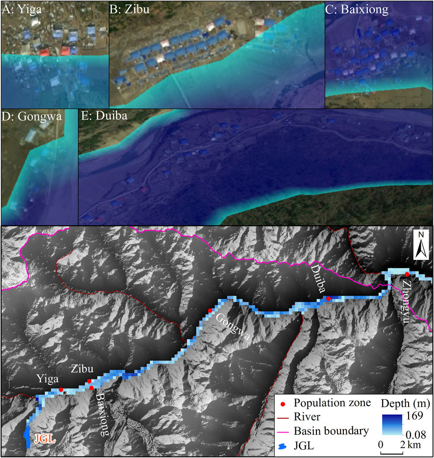
FIGURE 8. Maximum depth along the Niduzangbo river channel. Subfigure (A)–(E) are spatial distribution of maximum depth in different villages.

FIGURE 9

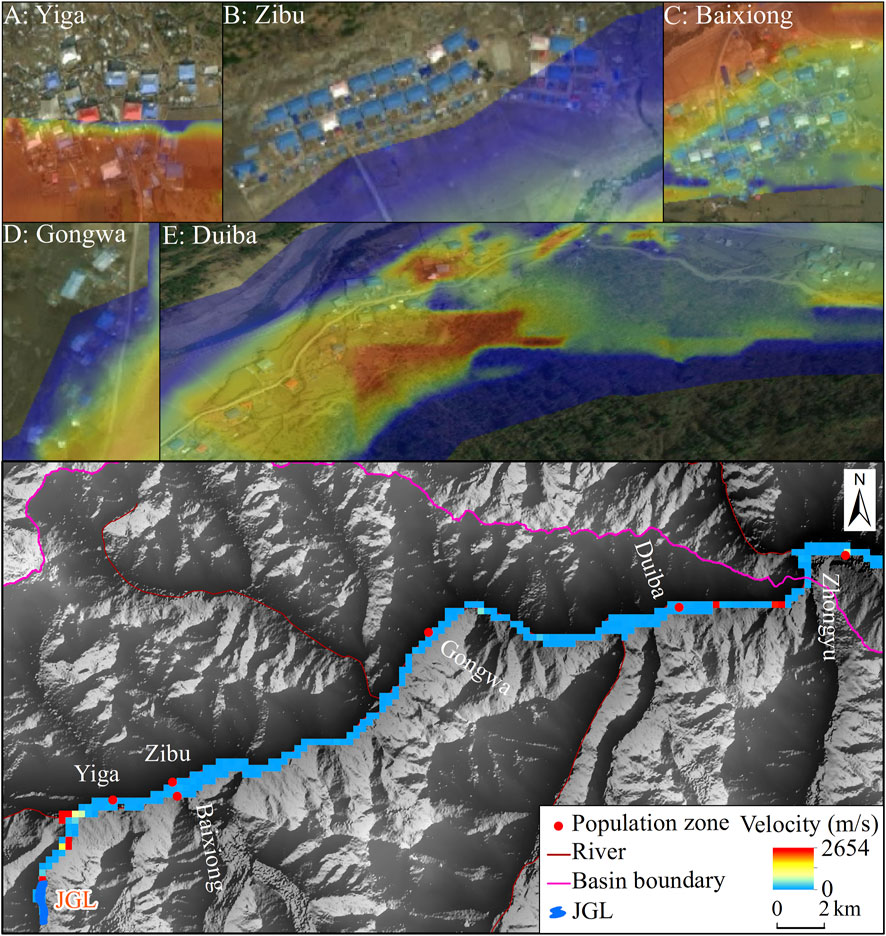
FIGURE 9. Maximum velocity along the Niduzangbo river channel. Subfigure (A)–(E) are spatial distribution of maximum velocity in different villages.

FIGURE 10

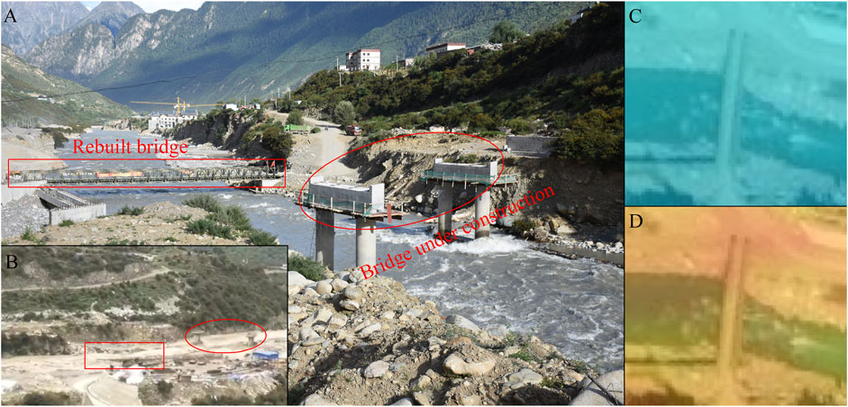
FIGURE 10. (A) is the photo of two bridges in Zhongyu town taken by Yao on 25 August 2020; (B) is the photo taken by inhabitants on 26 June 2020, these two bridges were damaged by flood; (C) is the maximum depth in the steel bridge; (D) is the maximum velocity in the steel bridge.

5 Discussion

5.1 The Reason of JGL Outburst

Glacial lakes are prone to outbursts under conditions of intense warming and heavy precipitation. In addition, ice/snow avalanches, glacier surge, and landslides can also result in GLOFs disaster (Yao et al., 2014; Wang et al., 2020). Global temperatures underwent a cold period (before 1980) and a warm period (after 1980) within the past 50 years (IPCC, 2021). Wang et al. (2021) reported the warming rate was −0.54°C/10a during 1961–1983 and changed to 0.12°C/10a in 1984–2020 in the study area, and there was a significant increase after 2000 (0.40°C/10a). Meanwhile, the average warming rate (8.28°C/10a) and precipitation (240 mm) in June 2020 (the month of the outburst) was higher than that (7.57°C/10a and 146 mm) during 1961–2020 (Wang et al., 2021). We also learned that the temperature in this area in June 2020 was significantly increased by the interview. Zheng et al. (2021) discovered that precipitation in the study area increased significantly in late May and June. The high temperature may result in the accelerated glacial melt and more glacial meltwater or ice entering the lake, the glacial lake is likely to burst if there is a heavy precipitation at this time. Therefore, the high temperature and extremely heavy precipitation before the moraine-failure was the main reason of this GLOF disaster.

The landslide of the lateral moraine was another cause of the JGL’s outburst (Liu et al., 2021; Wang et al., 2021; Zheng et al., 2021). The lateral moraine on the west side of the connection between JGL and its mother glacier occurred landslide on 21 June 2020. The landslide mass entering the JGL with a volume of 33 × 10⁴ m³ caused the water level to rise; the flow; velocity; and scour at the breach become more furious. There were different explanations on the lag between the dates of the landslide and the JGL’s outburst (Liu et al., 2021; Zheng et al., 2021). However, it can be confirmed that the landslide of the lateral moraine was the significant reason for the JGL’s outburst. The mother glacier’s termini connected to the JGL was stable before and after the outburst; thus, the possibility that this outburst caused by glacier surge or ice avalanche was excluded (Wang et al., 2021).

5.2 The Limitation of Modeling

We have the unique and valuable measured cross sections of Niduzangbo river-channels before JGL’s failure. The terrain data constructed from these measured cross sections were highly consistent with the real river-channel, which provided a great guarantee for the accuracy of the model. However, the flood propagation in the river-channel is very complicated. The flow can transform from clean-flow to sediment-bearing flow and then to debris-flow; such a transformation is often accompanied by processes such as sediment deposition and bank erosion by the flow (Nie et al., 2020). Many debris and rocks carried by the flood may temporarily block the narrower river-channel during transmission, acting as a dam, which consequently affects the timing of peak-flow transmission (Jain et al., 2012). In this study, the simulation of flood propagation in Niduzangbo river-channel was the process of solving the 2D Diffusion Wave equations using an implicit finite volume algorithm in the mapping 2D flow area. Although such simulation performance was proven to be competent for the reconstruction and simulation of GLOFs in previous studies (Anacona et al., 2015; Sattar et al., 2020), this result was not a perfectly authentic representation and just reflected the magnitude of the flood. There are three methods of modeling reservoir in HEC-RAS, namely 1D cross section, 2D grid, and linear reservoir hypothesis. The former two methods belong to standard hydraulic scope, but require bathymetric data with high precision. The linear reservoir hypothesis being suitable for the lack of the measured underwater terrain was adopted in this study. However, the shortcoming of this hypothesis is that the change in tilted water-surface and the backwater effect cannot be considered during reservoir discharging.

5.3 The Suggestion

Unmanned aerial vehicle (UAV) and unmanned vessel have been used widely for research related to glacier changes and disasters in recent years (Che et al., 2020), as they are not affected by complex terrain in alpine areas. These two techniques can yield the most genuine terrain data on the glacier surface, its surrounding and underwater with high spatial resolution, which can represent micro-geomorphic feature more amply and accurately (Che et al., 2020). Glaciers in the Niduzangbo basin have a steep tongue, such as the mother glacier of JGL, which has a slope of 45° between it and JGL (Wang et al., 2021). Therefore, it is promising to monitor the surface of glacier and glacial lake in this region by using UAV with 3D Lidar Scanner. The volume of the glacial lake is one of the most valuable information for assessing glacial-lake outburst risks and simulating GLOFs. Areas such as the Niduzangbo basin that experienced two GLOFs in recent decade require an integrated disaster prevention and mitigation plan. The government can work with research teams to measure the terrain of underwater, surrounding, and downstream channel of glacial lakes with high risk during low-rainfall periods using UAV and unmanned vessel. Then, the accurate topographic details can be obtained again by UAV after moraine-dam failure. These terrain data before and after the outburst are significant input parameters for conducting GLOFs simulation, allowing us to get more precise results and to improve our understanding on GLOFs. Finally, the knowledge about GLOFs is useful for developing disaster prevention and mitigation plans. In addition, we should reinforce the adoption of Synthetic Aperture Radar (SAR) image in glacial-lake research, because the landslide is a crucial reason of GLOFs and can be accurately monitored based on the SAR images.

6 Conclusion

The JGL has undergone a dramatic expansion toward its mother glacier in the past 30 years. The area, length, and volume of JGL increased by 0.20 ± 0.07 km², 0.66 ± 0.03 km, and 0.03 ± 0.005 km³ respectively from 1988 to 2020 (before the outburst). After the outburst, the corresponding values became 0.26 ± 0.03 km², 1.50 ± 0.02 km, and 0.01 ± 0.001 km³, respectively, which were 54, 21.9, and 81.2% less than that on 24 June 2020. Meanwhile, the area of its mother glacier was decreased by 1.42 km² (−0.44 km²/a) over 1988–2020.

The simulation of GLOF from JGL showed that approximately 0.05 km³ of water volume was discharged with the dropped water-level of 15.63 m after the outburst. The peak flow at the breach was 534.4 m³/s, and it arrived at the Zhongyu town after 3.86 h with a peak flow of 1,408.11 m³/s. The difference between the simulated and measured peak flows in Zhongyu town was 41.88 m³/s (3.53%), indicating the high accuracy of our simulation. When the flood arrived at the bridge connecting Zhongyu town and Ningzhonggang village, the maximum depth was 1.75 m and the maximum velocity was 6.73 m/s. For the villages along the river-channel between the JGL and Zhongyu town, Baixiong village and Duiba village were completely submerged when the flood arrived due to their proximity and similar elevation to the river; the hydraulic properties were 16.25 m and 4.74 m/s for the former respectively, 50.96 m and 6.98 m/s for the latter, respectively. The highest velocity was found in Yiga village (14.23 m/s), the lowest velocity occurred in Gongwa village (1.22 m/s), and the lowest depth was in Zibu village (1.94 m). The combination of landslide, high temperature, and extremely heavy precipitation resulted in this GLOF disaster.

Data Availability Statement

The raw data supporting the conclusions of this article will be made available by the authors, without undue reservation.

Author Contributions

XY designed this research and improved the manuscript. YZ and HD conducted the analysis. YZ wrote this manuscript. All authors contributed to the article and approved this submission.

Funding

National Natural Science Foundation of China (No. 41861013, No. 42071089, No. 42161027); National Key Research and Development Program of China (No. 2019YFE0127700); Open Research Foundation of National Cryosphere Desert Data Center (No. 20D02). The “Innovation Star” of Outstanding Graduate Student Program in Gansu Province (2021-CXZX-215); Northwest Normal University’s 2020 Graduate Research Grant Program (2020KYZZ001012).

Conflict of Interest

Author QW is employed by Northwest Engineering Cooperation Limited.

The remaining authors declare that the research was conducted in the absence of any commercial or financial relationships that could be construed as a potential conflict of interest.

Publisher’s Note

All claims expressed in this article are solely those of the authors and do not necessarily represent those of their affiliated organizations, or those of the publisher, the editors and the reviewers. Any product that may be evaluated in this article, or claim that may be made by its manufacturer, is not guaranteed or endorsed by the publisher.

Acknowledgments

Authors appreciate the USGS, CHEOS, ESA and NASA for their freely available satellite images. Zhongyu Hydrological Station are also acknowledged for providing us with the measured hydrological data during the outburst. YZ thanks XY and HD for their technical help and detailed guidance and advice during the preparation of this article.

References

Anacona, P. I., Mackintosh, A., and Norton, K. (2015). Reconstruction of a Glacial lake Outburst Flood (GLOF) in the Engaño Valley, Chilean Patagonia: Lessons for GLOF Risk Management. Sci. Total Environ. 527-528, 1–11. doi:10.1016/j.scitotenv.2015.04.096

PubMed Abstract | CrossRef Full Text | Google Scholar

Bhardwaj, A., Singh, M. K., Joshi, P. K., Snehmani, S. S., Singh, S., Sam, L., et al. (2015). A Lake Detection Algorithm (LDA) Using Landsat 8 Data: A Comparative Approach in Glacial Environment. Int. J. Appl. Earth Observation Geoinformation 38, 150–163. doi:10.1016/j.jag.2015.01.004

CrossRef Full Text | Google Scholar

Brunner, G. W. (2010). HEC-RAS (River Analysis System): User’s Mannual. New York, NY: Institute for Water Resource, Hydrological Engineering Center.

Google Scholar

Chanson, H. (2004). Hydraulics of Open Channel Flow. Second Edition. Oxford: Butterworth-Heinemann.

Google Scholar

Che, Y. J., Wang, S. J., and Liu, J. (2020). Application of Unmanned Aerial Vehicle (UAV) in the Glacier Region with Complex Terrain: A Case Study in Baishui River Glacier No.1 Located in the Yulong Snow Mountain. J. Glaciology Geocryology 42, 1391–1399. doi:10.7522/j.issn.1000-0240.2019.0002

CrossRef Full Text | Google Scholar

Chen, D. L., Xu, B. Q., Yao, T. D., Guo, Z. T., Cui, P., Chen, F. H., et al. (2015). Assessment of Past, Present and Future Environmental Changes on the Tibetan Plateau. Csb 60, 3025–3035. doi:10.1360/n972014-01370

CrossRef Full Text | Google Scholar

Duan, H., Yao, X., Zhang, D., Qi, M., and Liu, J. (2020). Glacial Lake Changes and Identification of Potentially Dangerous Glacial Lakes in the Yi'ong Zangbo River Basin. Water 12, 538–553. doi:10.3390/w12020538

CrossRef Full Text | Google Scholar

Frey, H., Haeberli, W., Linsbauer, A., Huggel, C., and Paul, F. (2010). A Multi-Level Strategy for Anticipating Future Glacier Lake Formation and Associated Hazard Potentials. Nat. Hazards Earth Syst. Sci. 10, 339–352. doi:10.5194/nhess-10-339-2010

CrossRef Full Text | Google Scholar

Hall, D. K., Bayr, K. J., Schöner, W., Bindschadler, R. A., and Chien, J. Y. L. (2003). Consideration of the Errors Inherent in Mapping Historical Glacier Positions in Austria from the Ground and Space (1893-2001). Remote Sensing Environ. 86, 566–577. doi:10.1016/S0034-4257(03)00134-2

CrossRef Full Text | Google Scholar

Horritt, M. S., and Bates, P. D. (2002). Evaluation of 1D and 2D Numerical Models for Predicting River Flood Inundation. J. Hydrol. 268, 87–99. doi:10.1016/S0022-1694(02)00121-X

CrossRef Full Text | Google Scholar

Huggel, C., Kääb, A., Haeberli, W., Teysseire, P., and Paul, F. (2002). Remote Sensing Based Assessment of Hazards from Glacier Lake Outbursts: A Case Study in the Swiss Alps. Can. Geotech. J. 39, 316–330. doi:10.1139/t01-099

CrossRef Full Text | Google Scholar

IPCC (2021). Climate Change 2021: The Physical Science Basis: Contribution of Working Group I to the Fifth Assessment Report of the Intergovernmental Panel on Climate Change. Cambridge: Cambridge University Press.

Google Scholar

Jain, S. K., Lohani, A. K., Singh, R. D., Chaudhary, A., and Thakural, L. N. (2012). Glacial Lakes and Glacial Lake Outburst Flood in a Himalayan Basin Using Remote Sensing and GIS. Nat. Hazards. 62, 887–899. doi:10.1007/s11069-012-0120-x

CrossRef Full Text | Google Scholar

Jia, Y., and Cui, P. (2020). The Extreme Climate Background for Glacial Lakes Outburst Flood Events in Tibet. Clim. Change Res. 16, 396–404. doi:10.12006/j.issn.1673-1719.2019.181

CrossRef Full Text | Google Scholar

Li, J., and Sheng, Y. (2012). An Automated Scheme for Glacial Lake Dynamics Mapping Using Landsat Imagery and Digital Elevation Models: A Case Study in the Himalayas. Int. J. Remote Sensing 33, 5194–5213. doi:10.1080/01431161.2012.657370

CrossRef Full Text | Google Scholar

Liu, C., Mayor-Mora, R., Sharma, C. K., Xing, H., and Wu, S. (1988). Report on First Expedition to Glaciers and Glacier Lakes in the Pumqu (Arun) and Poiqu (Bhote-Sun Kosi) River Basins, Xizang (Tibet), China : Sino-Nepalese Investigation of Glacier Lake Outburst Floods in the Himalayas. Beijing: Science Press.

Google Scholar

Liu, J. K., Zhou, L. X., Zhang, J. J., and Zhao, W. Y. (2021). Characteristics of Mechanism of Jiwengco Glacial Lake Flood Outburst in Tibet. Geol. Rev. 67, 17–18. doi:10.16509/j.georeview.2021.s1.007

CrossRef Full Text | Google Scholar

López-Moreno, J. I., Valero-Garcés, B., Mark, B., Condom, T., Revuelto, J., Azorín-Molina, C., et al. (2017). Hydrological and Depositional Processes Associated with Recent Glacier Recession in Yanamarey Catchment, Cordillera Blanca (Peru). Sci. Total Environ. 579, 272–282. doi:10.1016/j.scitotenv.2016.11.107

PubMed Abstract | CrossRef Full Text | Google Scholar

Loriaux, T., and Casassa, G. (2013). Evolution of Glacial Lakes from the Northern Patagonia Icefield and Terrestrial Water Storage in a Sea-Level Rise Context. Glob. Planet. Change 102, 33–40. doi:10.1016/j.gloplacha.2012.12.012

CrossRef Full Text | Google Scholar

Lv, R. R., and Li, D. J. (1986). Debris Flow Induced by Lce Lake Burst in the Tangbulang Gully,Gongbujiangda, Xizang (Tibet). J. Glaciology Geocryology 8, 61–71.

Google Scholar

Ma, J., Song, C., and Wang, Y. (2021). Spatially and Temporally Resolved Monitoring of Glacial Lake Changes in Alps during the Recent Two Decades. Front. Earth Sci. 9, 1–11. doi:10.3389/feart.2021.723386

CrossRef Full Text | Google Scholar

McFeeters, S. K. (1996). The Use of the Normalized Difference Water Index (NDWI) in the Delineation of Open Water Features. Int. J. Remote Sensing 17, 1425–1432. doi:10.1080/01431169608948714

CrossRef Full Text | Google Scholar

Nie, N., Zhang, W. C., and Deng, C. (2012). Spatial and Temporal Climate Variations from 1978 to 2009 and Their Trend Projection over the Yarlung Zangbo River Basin. J. Glaciology Geocryology 34, 64–71.

Google Scholar

Nie, Y., Liu, Q., Wang, J., Zhang, Y., Sheng, Y., and Liu, S. (2018). An Inventory of Historical Glacial Lake Outburst Floods in the Himalayas Based on Remote Sensing Observations and Geomorphological Analysis. Geomorphology 308, 91–106. doi:10.1016/j.geomorph.2018.02.002

CrossRef Full Text | Google Scholar

Nie, Y., Liu, W., Liu, Q., Hu, X., and Westoby, M. J. (2020). Reconstructing the Chongbaxia Tsho Glacial Lake Outburst Flood in the Eastern Himalaya: Evolution, Process and Impacts. Geomorphology 370, 1–14. doi:10.1016/j.geomorph.2020.107393

CrossRef Full Text | Google Scholar

Qin, D. H. (2014). Dictionary of Cryosphere Science. Beijing: China Meteorological Press.

Google Scholar

Richardson, S. D., and Reynolds, J. M. (2000). An Overview of Glacial Hazards in the Himalayas. Quat. Int. 65-66, 31–47. doi:10.1016/S1040-6182(99)00035-X

CrossRef Full Text | Google Scholar

Sattar, A., Goswami, A., and Kulkarni, A. V. (2019). Correction to: Application of 1D and 2D Hydrodynamic Modeling to Study Glacial Lake Outburst Flood (GLOF) and its Impact on a Hydropower Station in Central Himalaya. Nat. Hazards. 98, 817. doi:10.1007/s11069-019-03747-5

CrossRef Full Text | Google Scholar

Sattar, A., Goswami, A., Kulkarni, A. V., and Emmer, A. (2020). Lake Evolution, Hydrodynamic Outburst Flood Modeling and Sensitivity Analysis in the Central Himalaya: A Case Study. Water 12, 237–256. doi:10.3390/w12010237

CrossRef Full Text | Google Scholar

Sattar, A., Goswami, A., and Kulkarni, A. V. (2019). Hydrodynamic Moraine-Breach Modeling and Outburst Flood Routing - A Hazard Assessment of the South Lhonak Lake, Sikkim. Sci. Total Environ. 668, 362–378. doi:10.1016/j.scitotenv.2019.02.388

PubMed Abstract | CrossRef Full Text | Google Scholar

Sattar, A., Haritashya, U. K., Kargel, J. S., Leonard, G. J., Shugar, D. H., and Chase, D. V. (2021). Modeling Lake Outburst and Downstream Hazard Assessment of the Lower Barun Glacial Lake, Nepal Himalaya. J. Hydrol. 598, 126208–126222. doi:10.1016/j.jhydrol.2021.126208

CrossRef Full Text | Google Scholar

Shangguan, D. H., Liu, S. Y., Ding, L. F., Zhang, S. Q., Li, G., and Zhang, Y. (2008). Variation of Glaciers in the Western NyainqÉNtanglha Range of Tibetan Plateau during 1970-2000. J. Glaciology Geocryology 30, 204–210.

Google Scholar

Sun, M. P., Liu, S. Y., Yao, X. J., and Li, L. (2014). The Cause and Potential Hazard of Glacial Lake Outburst Flood Occurred on July 5, 2013 in Jiali County, Tibet. J. Glaciology Geocryology 36, 158–165. doi:10.7522/j.issn.1000-0240.2014.0020

CrossRef Full Text | Google Scholar

Tong, L. Q., Qi, S. W., An, G. Y., and Liu, C. L. (2019). Remote Sensing Investigation of Major Geological Disasters in the Himalayas. J. Eng. Geology. 27, 496. doi:10.3969/j.issn.1004-9665.2014.04.022

CrossRef Full Text | Google Scholar

Veh, G., Korup, O., von Specht, S., Roessner, S., and Walz, A. (2019). Unchanged Frequency of Moraine-Dammed Glacial Lake Outburst Floods in the Himalaya. Nat. Clim. Chang. 9, 379–383. doi:10.1038/s41558-019-0437-5

CrossRef Full Text | Google Scholar

Wang, S., Che, Y., and Xinggang, M. (2020). Integrated Risk Assessment of Glacier lake Outburst Flood (GLOF) Disaster over the Qinghai-Tibetan Plateau (QTP). Landslides 17, 2849–2863. doi:10.1007/s10346-020-01443-1

CrossRef Full Text | Google Scholar

Wang, S., Yang, Y., Gong, W., Che, Y., Ma, X., and Xie, J. (2021). Reason Analysis of the Jiwenco Glacial Lake Outburst Flood (GLOF) and Potential Hazard on the Qinghai-Tibetan Plateau. Remote Sensing 13, 1–11. doi:10.3390/rs13163114

CrossRef Full Text | Google Scholar

Xiang, L. Z., Liu, Z. H., Liu, J. B., Li, L., Zou, X., Lou, M. Y., et al. (2013). Variation of Glaciers and Lts Response to Climate Change in Bomi County of Tibet Autonomous Region in 1980-2010. J. Glaciology Geocryology 35, 593–600. doi:10.7522/j.issn.1000-0240.2013.0068

CrossRef Full Text | Google Scholar

Xin, W., Shiyin, L., Wanqin, G., Xiaojun, Y., Zongli, J., and Yongshun, H. (2012). Using Remote Sensing Data to Quantify Changes in Glacial Lakes in the Chinese Himalaya. Mountain Res. Dev. 32, 203–212. doi:10.1659/MRD-JOURNAL-D-11-00044.1

CrossRef Full Text | Google Scholar

Xu, D. M., and Feng, Q. H. (1989). Dangerous Glacial Lake and Outburst Features in Xizang Himalayas. Acta Geogr. Sinica 3, 1–11.

Google Scholar

Yao, T. D., Yu, W. S., Wu, G. J., Xu, B. Q., Yang, W., Zhao, H. B., et al. (2019). Glacier Anomalies and Relevant Disaster Risks on the Tibetan Plateau and Surroundings. Chinse Sci. Bull. 64, 2770–2782. CNKI:SUN:KXTB.0.2019-27-004. doi:10.1016/j.scib.2019.03.033

CrossRef Full Text | Google Scholar

Yao, T., Thompson, L. G., Mosbrugger, V., Zhang, F., Ma, Y., Luo, T., et al. (2012). Third Pole Environment (TPE). Environ. Dev. 3, 52–64. doi:10.1016/j.envdev.2012.04.002

CrossRef Full Text | Google Scholar

Yao, X. J., Liu, S. Y., Sun, M. P., and Zhang, X. J. (2014). Study on the Glacial Lake Outburst Flood Events in Tibet since the 20th Century. J. Nat. Resour. 29, 1377–1390. doi:10.11849/zrzyxb.2014.08.010

CrossRef Full Text | Google Scholar

Yao, X. J., Liu, S. Y., Zhu, Y., Gao, Y. P., An, L. N., and Li, X. F. (2015). Design and Implementation of an Automatic Method for Deriving Glacier Centerlines Based on GIS. J. Glaciology Geocryology 37, 1563–1570. doi:10.7522/j.issn.1000-0240.2015.0173

CrossRef Full Text | Google Scholar

Yao, X., Liu, S., Sun, M., Wei, J., and Guo, W. (2012). Volume Calculation and Analysis of the Changes in Moraine-Dammed Lakes in the North Himalaya: A Case Study of Longbasaba Lake. J. Glaciol. 58, 753–760. doi:10.3189/2012JoG11J048

CrossRef Full Text | Google Scholar

Zheng, G., Mergili, M., Emmer, A., Allen, S., Bao, A., Guo, H., et al. (2021). The 2020 Glacial Lake Outburst Flood at Jinwuco, Tibet: Causes, Impacts, and Implications for Hazard and Risk Assessment. The Cryosphere 15, 3159–3180. doi:10.5194/tc-15-3159-2021

CrossRef Full Text | Google Scholar

Zhou, L. X., Liu, J. K., and Li, Y. L. (2020). Calculation Method of Mathematical Model of the Moraine Dammed Lake Storage Capacity. Sci. echnology Eng. 20, 9804–9809. doi:10.3969/j.issn.1671-1815.2020.24.016

CrossRef Full Text | Google Scholar