FC-ZSM: Spatiotemporal Downscaling of Rain Radar Data Using a Feature Constrained Zooming Slow-Mo Network

Introduction

Downscaling forecasting is an important means for refined forecasting of meteorological elements in space or time dimensions. Commonly, the downscaling technology refers to the conversion which turns meteorological low-resolution data (large-scaled numerical matrix) into high-resolution information (small-scaled numerical matrix) under the same region. Downscaling can be divided into two dimensions: space and time. Spatial downscaling is the most extensive behavior of refined forecasting, while the method of temporal downscaling still needs to be studied (Maraun et al., 2010; Lee and Jeong, 2014; Monjo, 2016; Sahour et al., 2020). Early spatial downscaling techniques are implemented by using interpolation algorithms (Lanza et al., 2001) or statistical models. Interpolation algorithms contain linear interpolation, bilinear interpolation, nearest neighbor interpolation, and trilinear interpolation. The value of each pixel on the image is calculated by building the distance relationship of several pixels around it. The statistical model learns a corresponding function from data pairs which include low-resolution and high-resolution precipitation to observe a particular distribution. However, meteorological observation data are a kind of structural information (Berg et al., 2013; Yao et al., 2016). It means that meteorological data are time-series data; the data from different regions have diverse latitude and longitude coordinates, and these kinds of data can be influenced by associated meteorological element data. These factors make downscaling behavior susceptible to the influence of meteorological observations in their vicinity (Beck et al., 2019). Because of this, early interpolation methods do not make good use of this information; statistical methods are limited by empirical knowledge of time stationarity assumptions, control theory, and prediction theory.

In recent years, deep learning has become increasingly popular in climate science as the demand for high-resolution climate data from emerging climate studies have increased (Prein et al., 2015). Since the problem of downscaling meteorological data is similar to the image super-resolution problem of computer vision, the networks in the field of vision have been often seen as the main architecture to deal with the downscaling problem. However, the meteorological downscaling problem is different from the simple image super-resolution problem. For example, as a kind of structural information, the downscaling of meteorological data will be constrained by the implicit rules of static data such as terrain, vegetation, longitude, and latitude (Vandal et al., 2017; Serifi et al., 2021). Dynamic data which include air pressure, temperature, and humidity often have corrective effects on downscaling results. The threshold range of meteorological values is distinguished from the image’s pixel intensity threshold range. Meteorological data are usually not integer data. They have strong randomness which makes their upper and lower thresholds difficult to determine. These problems are obviously not needed to be considered in image problems, and it makes the problem of meteorological downscaling seem more complex.

In the field of image super-resolution, early networks are dominated by lightweight convolutional neural networks such as the super-resolution convolutional neural network (SRCNN) (Ward et al., 2017), fast super-resolution convolutional neural network (FSRCNN) (Zhang and Huang, 2019), and very deep convolutional network for super-resolution (VDSR) (Lee et al., 2019). The effect of these networks reconstructing the original image is generally better than that of ordinary interpolation methods. Although the lightweight models make the frame rate of this type of network operation faster, they still limit the reconstruction effect of the image. To solve this problem, the U-shaped structural neural network (U-Net) is used, and a GAN structure is then applied to the task. Structural variants that use low-resolution images as inputs were proposed by Mao et al. (2016) and Lu et al. (2021), and their network structures are built on the classic network which is called the U-Net (Ronneberger et al., 2015). Their data are reconstructed from different resolutions by taking advantage of the multi-scale characteristics of the network, and finally, their results are great. In addition, since the use of generative adversarial networks (GANs) proposed by Wang et al. (2018), a variant of the GAN structure SSR-TVD (Han et al., 2020) has been proposed to solve spatial super-resolution problems. The GAN is a self-supervised learning method. It takes the form of modeling data distribution to generate a possible interpretation which uses a generative network for sampling and then generates fuzzy compromises by discriminating networks. This structure can produce some specious details which can be seen truly as the ground truth. From the indicator, the effect is wonderful, but whether there exists false information is still worth discussing.

In the field of meteorological downscaling, the DeepSD network (a generalized stacked SRCNN) was proposed by Vandal et al. (2017). In this work, to take structural information into consideration, they made additional variables spliced with input features in a channel dimension before convolution. Then, they used convolution to aggregate structural relationships. The additional variables included geopotential height and forecast surface roughness. Finally, they achieved improvements in the task of downscaling. Rodrigues et al. used a CNN (convolutional neural network) to combine and downscale multiple ensemble runs spatially, and their approach can make a standard CNN give blurry results (Rodrigues et al., 2018). Pan used the convolution layer and full connection layer to connect the input and output with a network to predict the value of each grid point (Pan et al., 2019) without considering regional issues. These lightweight neural network methods verify that deep learning downscaling is feasible. Compared with the traditional methods, the deep learning method can get better results in a limited research area. In our work, we do not adopt a lightweight network. Since a lightweight network can get a great effect in spatial downscaling, it cannot deal with temporal downscaling. A common reason for it being unfit is that there does not exist a sequence processing module which can deal with the interpolation of temporal information. Methods like DeepSD, VDSR, and FSRCNN are designed for dealing with single data super-resolution, and most of these structures which are designed with a residual network cannot be adapted to the temporal downscaling problem. Their performances are correspondingly weak without the help of timing information. But the idea of taking additional variables into consideration is desirable, and we followed and further improved this method.

Commonly, the update frame rate of meteorological data is usually much lower than the video frame rate, and the meteorological early warning has higher requirements for numerical accuracy. Therefore, the index performance of the network should be placed in the first place. Höhlein studied a variety of structures for spatial downscaling of wind speed data, including U-Net architecture and U-Net with a residual structure which yielded better results (Höhlein et al., 2020). Adewoyin proposed TRU-NET (a U-Net variant structure) to downscale high-resolution images of precipitation spatially (Adewoyin et al., 2021). Sha proposed the Nest-UNet structure to downscale the daily precipitation image (Sha et al.,2020). The network is more densely connected based on the U-Net structure and has achieved good results. Serifi tested the low-frequency temperature data and high-frequency precipitation data by using the U-Net architecture based on the three-dimensional convolution. To take structural information into consideration, Serifi put values which include time, latitude and longitude coordinates, and terrain data into a network from a different scale. The way of fusion is the same as DeepSD. The results showed that an RPN (a U-shaped structure with a residual structure) is more suitable for the downscaling of low-frequency data, and a DCN (the network without a residual structure) is more suitable for the downscaling of high-frequency data. It can be seen that the mainstream networks adopted to deal with downscaling problems in recent years are almost using the U-Net as the basic architecture. Only a small number of solutions are based on the GAN and long short-term memory network (LSTM) structures (Tran Anh et al., 2019; Stengel et al., 2020; Accarino et al., 2021). It means that the U-Net is the mainstream supervised learning method for deep learning to solve the problem of meteorological downscaling. The U-Net structure has the advantages of a symmetrical network structure, moderate size, diverse improvement methods, and multi-scale feature analysis characteristics. But there are still some problems which are as follows:

1) The processing of time-series characteristics in the U-Net network adopts the method of spatializing the time dimension. This processing method conforms to the principle of image optical flow, but the time-series relationship in the real environment is different from the spatial relationship, which is more similar to the iterative relationship of a complex system.

2) The network input data feature types and the fusion methods are single. There is no difference between fusion methods for different types of data.

To address the aforementioned issues, in this study, we proposed a Feature Constrained Zooming Slow-Mo network, which has four modules: the feature extraction module, frame feature time interpolation module, deformable ConvLSTM module, and high-resolution frame reconstruction module. Compared with the U-Net series network, our network can extend channel dimensions. This feature makes it possible to take dynamic parallel data into channel dimensions as a factor, and the time information is delivered to the ConvLSTM. Furthermore, we considered a new strategy to extract static data features by deformable convolution. These strategies make our networks perform more scientifically in a multi-feature fusion.

The contributions of this study to the downscaling problem are as follows:

1) A deep learning downscaling method based on the convolutional LSTM (Xingjian et al., 2015) structure which can simultaneously solve both temporal and spatial downscaling problems is given.

2) Static data and dynamic data are introduced as influence characteristics, and the types of feature fusions are enriched.

3) This study proposes a method for constructing a feature blender using the deformable convolution, which enriches the feature fusion method.

Preliminaries

Formulation of the Downscaling Problem

The downscaling problem of meteorological elements is usually divided into two parts: spatial downscaling and temporal downscaling. Spatial downscaling problems can be regarded as follows:

Given the three-dimensional grid data $\left(t,m,n\right)$ and the magnification factors $k_{x}and{k}_y$, using algorithms to fill the grid data to $\left(t,k_x\cdot m,k_y\cdot n\right)$ by taking advantage of the relevance of spatiotemporal data information.

The temporal downscaling problem is roughly similar to the spatial downscaling problem. It needs to set a time scale magnification factor $k_t$ to enlarge the raster data to $\left(k_t\cdot t,m,n\right)$. Different from the spatial downscaling problem, when dealing with data like precipitation, high-frequency data will be aggregated. As a result, in the process of downscaling, there are problems such as data block’s position transformation and numerical dynamic changes. Therefore, the optical flow needs to be considered (Sun et al., 2021).

Commonly, the downscaling problem can be understood as the inverse process of data coarsening, which is shown in Eq. 1, where $X$ is low-resolution data, $Y$ is high-resolution data, and $f$ is the data coarsening function. The data coarsening operation is usually achieved by interpolation, pooling operation, or acquisition from the real environment.

$\underset{coarsening}{\underbrace{X=f\left(Y\right)}},\underset{downscaling}{\underbrace{Y=f^{-1}\left(X\right)}},(1)$

Zooming Slow-Mo Network

One-stage Zooming Slow-Mo (Xiang et al., 2020) is a network combined with ConvLSTM and deformable convolution networks (Dai et al., 2017), which is designed to generate high-resolution slow-motion video sequences. The structure of the network is shown in Figure 1. It consists of four parts: the feature extraction module, frame feature time interpolation module, deformable ConvLSTM module, and high-resolution frame reconstruction module. First of all, a feature extractor with one convolution layer and $k_1$ residual blocks is used to extract features. Then, the frame feature time interpolation module with deformable convolution is used to synthesize the low-resolution feature map of the intermediate frame by taking the feature map as the input. Afterward, to make better use of the time information, the deformable ConvLSTM module is used to process the continuous feature map, and this operation makes the feature images aligned and aggregated at the same time. Finally, the high-resolution reconstruction module is used to reconstruct the aggregated feature images.

FIGURE 1

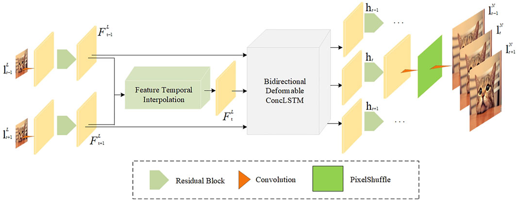
FIGURE 1. One-stage Zooming Slow-Mo network.

Different from other networks only for spatial downscaling and U-Net, the structure of our network constructs modules separately for each super-resolution step. The most important change is that our network has a frame feature time interpolation module and deformable ConvLSTM module because it is common to see similar structures like a feature extraction module and high-resolution reconstruction module in most networks for spatial downscaling. These two modules provide a new view of generating a middle frame and applying ConvLSTM, which is a popular scheme for deep learning timing problems. The frame feature time interpolation module changed the use of stacked convolutions singly to solve the frame interpolation problem. With deformable convolution’s help, the middle frame can be generated more precisely. The deformable ConvLSTM module changed the use of stacked convolutions singly to solve the timing problem; hence, every downscaling array can completely fuse temporal sequence information by the mechanism of long short-term memory.

Frame Feature Time Interpolation Module

As shown in Figure 2, after feature extraction, the feature maps $F_1^L$ and $F_3^L$ are obtained. The traditional method performs interpolation on the time scale of pixel-level frames, but such an operation will make the front and back network structures be separated into two neural networks. Different from this method, Zooming Slow-Mo is designed to train a time interpolation function $f(\cdot )$ by using convolution to directly synthesize an intermediate feature map $F_2^L$. The general expression of this interpolation function is as follows:

$F_2^L=f\left(F_1^L,F_3^L\right)=H\left(T_1\left(F_1^L,{\text{Φ}}_1\right),T_3\left(F_3^L,{\text{Φ}}_3\right)\right),(2)$

FIGURE 2

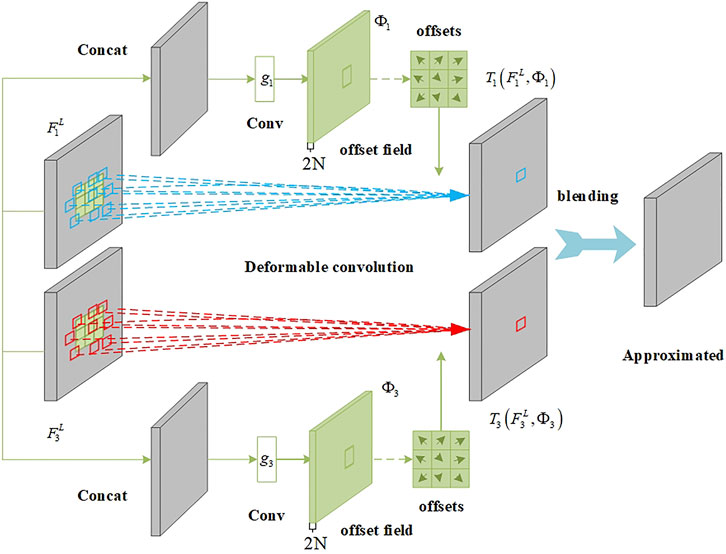
FIGURE 2. Frame feature time interpolation module.

Among them, $T_1(\cdot )$ and $T_3(\cdot )$ are two sampling functions. ${\mathrm{\Phi }}_1$ and ${\mathrm{\Phi }}_3$ are the corresponding sampling parameters. $H(\cdot )$ is a hybrid function for aggregating the sampling features.

To precisely generate $F_2^L$, $T_1(\cdot )$ needs to capture forward motion information between $F_1^L$ and $F_2^L$, and $T_3(\cdot )$ needs to capture the backward motion information between $F_2^L$ and $F_3^L$. Since $F_2^L$ does not exist in the input data, the forward and backward motion information cannot be obtained directly. The motion information between $F_1^L$ and $F_3^L$ is used to approximate the forward and backward motion information. Furthermore, deformable convolution is used to capture the motion information of the frame feature time interpolation module from the position relationship and mapping relationship. The sampling method based on deformable convolution can explore more abundant local time content and motion relationship.

$T_1(\cdot )$ and $T_3(\cdot )$ have the same network design structure, but their network weights are different. Taking $T_1(\cdot )$ as an example, it maps the low-resolution frame features $F_1^L$ and $F_3^L$ as input to predict the sampling offset of $F_1^L$:

$\text{Δ}{p}_1=g_1\left(\left[F_1^L,F_3^L\right]\right),(3)$

In this formula, $\Delta p_1$ is a learnable offset and also refers to the sampling parameters ${\Phi }_1$. $g_1$ represents a general function of several convolution layers. $[,]$ represents the connected channels. With a learnable offset, deformable convolution can be used:

$T_1\left(F_1^L,{\text{Φ}}_1\right)=DConv\left(F_1^L,\text{Δ}{p}_1\right),(4)$

Applying the same method, we can obtain $\text{Δ}{p}_3=g_3\left(\left[F_3^L,F_1^L\right]\right)$ and the sampled features $T_3\left(F_3^L,{\text{Φ}}_3\right)$ by deformable convolution.

To mix two sampling features, the network uses the simple linear mixing function $H(\cdot )$:

$F_2^L=\alpha \ast T_1\left(F_1^L,{\text{Φ}}_1\right)+\beta \ast T_3\left(F_3^L,{\text{Φ}}_3\right),(5)$

In this formula, $\alpha$ and $\beta$ are two learnable $1\times 1$ convolutional kernels. $\ast$ is a convolutional operator. Since the composite low-resolution feature map $F_2^L$ will be used to predict the intermediate high-resolution frame $I_2^H$, it will enforce the synthesized LR feature map to be close to the real intermediate low-resolution feature map. Therefore, the two offsets $\Delta p_1$ and $\Delta p_3$ will implicitly learn to capture the forward and backward motion information, respectively.

Deformable ConvLSTM

ConvLSTM is a two-dimensional sequence data modeling method that is used here for aggregation on the temporal dimension. At the time point $t$, ConvLSTM updates the hidden layer $h_t$ and the cell layer $c_t$, and the formula is as follows:

$h_t,c_t=ConvLSTM\left(h_{t-1},c_{t-1},F_t^L\right),(6)$

As is seen from the state update mechanism here, ConvLSTM can only implicitly capture the state of motion between previous states: $h_{t-1}$, $c_{t-1}$ and input feature maps with small convolutional receptive fields. Therefore, if there is a large change between consecutive frames, the previous state will not match the time scale that $F_t^L$ produces seriously. Then, the mismatched noise information that will be propagated by $h_{t-1}$ and $c_{t-1}$ is not the global information on the useful time scale. As a result, the reconstructed high-resolution image will produce artifacts with probability.

To solve this problem and effectively obtain global time scale information, the network adds a deformable convolution operation to the state update process of $h_t$ and $c_t$ in ConvLSTM. As shown in Figure 3, the update mechanism of ConvLSTM becomes

$\begin{array}{l}\text{Δ}{p}_t^h=g^h\left(\left[h_{t-1},F_t^L\right]\right),\\ \text{Δ}{p}_t^c=g^c\left(\left[c_{t-1},F_t^L\right]\right),\\ h_{t-1}^a=DConv\left(h_{t-1},\text{Δ}{p}_t^h\right),\\ c_{t-1}^a=DConv\left(c_{t-1},\text{Δ}{p}_t^c\right),\\ h_t,c_t=ConvLSTM\left(h_{t-1}^a,c_{t-1}^a,F_t^L\right),\end{array}(7)$

FIGURE 3

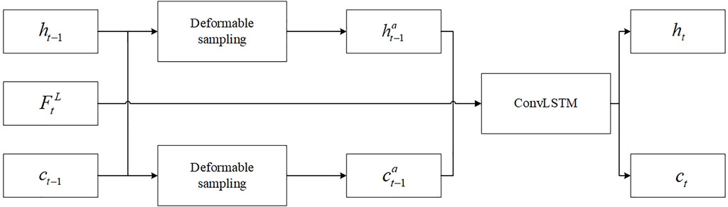
FIGURE 3. Deformable ConvLSTM.

Among them, $g^h$ and $g^c$ are the general functions with the stacked convolutional layers, $\Delta p_t^h$ and $\Delta p_t^c$ are the predicted offsets, $h_{t-1}^a$ and $c_{t-1}^a$ are the aligned hidden and cell states, respectively. Compared with the normal ConvLSTM, the hidden layer $h_{t-1}^a$ and the cell layer $c_{t-1}^a$ are forced to align with the input features $F_t^L$ in the deformable ConvLSTM, which enables it to handle motion in the video. In addition, the ConvLSTM here uses a bidirectional structure, which can fully obtain the information transmitted forward and backward. Finally, the hidden layer $h_t$ is used as the output, and the frame reconstruction module is used as the input.

Frame Reconstruction

To reconstruct high-resolution video frames, a synthetic network shared on a time scale is used. It takes a single hidden state $h_t$ as input and outputs the corresponding high-resolution frame. The network first uses ${\text{k}}_2$-stacked residual blocks to learn the depth features and finally uses a sub-pixel upscaling module (Shi et al., 2016), as shown in Figure 4 to reconstruct high-resolution frames.

FIGURE 4

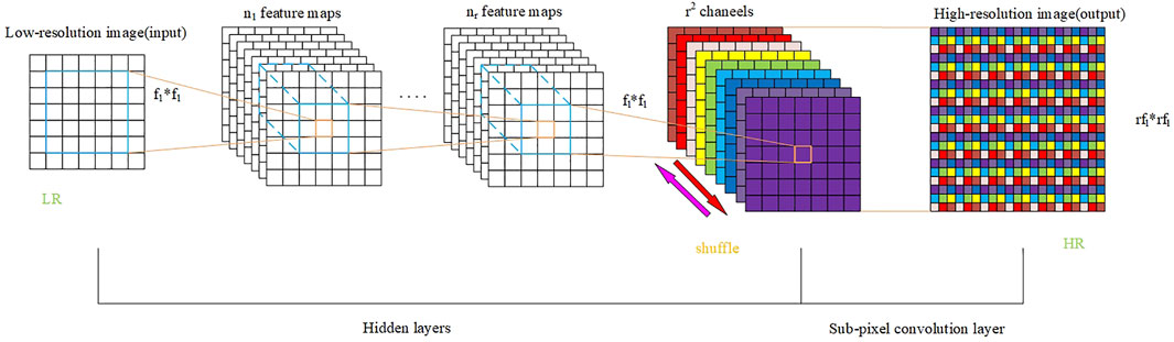
FIGURE 4. Sub-pixel upscaling module.

The Model

The model presented in this article uses the Zooming Slow-Mo network as the infrastructure. Although the network has proven to be quite powerful in image super-resolution missions, the data complexity of meteorological downscaling missions and the multiple input data sources make the original architecture unable to be directly adapted. To address this issue, we classified the input data and reconstructed the Feature Constrained Zooming Slow-Mo network, which is shown in Figure 5, by using the characteristics of deformable convolution.

FIGURE 5

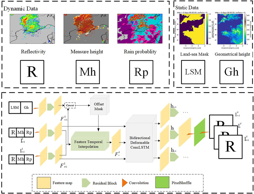
FIGURE 5. Feature constrained Zooming Slow-Mo network. Dynamic data use the situation from southeast of France as an example just for showing three kinds of dynamic data, and we used data from northwest of France in our experiment. Static data are the real data from northwest of France.

Selection of Dynamic and Static Data

Different from video super-resolution or simple image super-resolution, the problem of actual data association is usually considered in the meteorological downscaling behavior. When it comes to precipitation, it is natural to be associated with factors of precipitation conditions. For example, the probability of precipitation is a factor which can be taken into consideration. To enrich the dynamic data, we also added the element of reflectivity measurement height. In addition to these dynamic data, static data are always considered as influencing factors which include latitude and longitude coordinates, terrain height, and vegetation information (Ceccherini et al., 2015). Since the adopted data set is obtained in the northwest of France, there is a difference between sea and land. We believe that geometrical height information and sea-land mask are the main and easily available static influence factors. Therefore, we selected the geometrical height and land–sea mask as static influence factors.

Feature Blender

The fusion of data is a problem worth considering for Zooming Slow-Mo. The reasons are as follows:

1) Jumping out of the U-Net framework and lacking the support of symmetrical structure, it is no longer applicable to integrate information into small-scale features.

2) There are two types of data in the existing data: static data and dynamic data. If the violent channel superposition method is adopted, the effect of integration will naturally get a big discount.

As we can see from the aforementioned reasons, the application of a new network structure leads to the difficulty of designing a feature blender. The most important factor is that static data and dynamic data are two types of data. It means that it is unreasonable to fuse two kinds of data in the same way. Therefore, the question as to how to design the feature blender remains unexplored.

In the network structure of Zooming Slow-Mo, there exists an important component which is called deformable convolution. Deformable convolution improves its performance by resetting the position information compared to common convolution. The process of resetting position information can be seen as a shift of the convolutional kernel scope. In fact, the behavior of the shift is before the convolution mapping. Since this behavior does not belong to the convolution process, we can interpret it as a process of making a position rule. Different from dynamic data, static data are fixed values. When it comes to dynamic data, we expect these data can make effect on correcting the downscaling value. Therefore, the question as to what kind of information can be extracted from a fixed value is yet to be explored. In our opinion, static data are the key to making the position rule.

According to the idea that dynamic data help correct results and static data help make position rules, we made some structural changes to the network, which is shown in Figure 6. Since reflectivity itself is dynamic data, we put three kinds of dynamic data into the feature extractor in the form of channel stacking. Then, we added a new static data feature extractor on the basis of the original network, which forms a parallel relationship with the dynamic data feature extractor. Considering that putting a full static data feature map into the offset leads to the position rule being fixed, we spliced equal amounts of the static feature map and dynamic feature map together in a channel dimension. Therefore, the acquisition method of offset $\Delta p$ becomes ($F_S$ is a feature map of static data)

$\text{Δ}p=g\left(\left[F_1^L,F_3^L,F_S\right]\right),(8)$

FIGURE 6

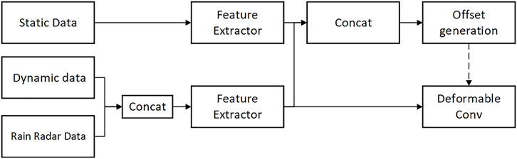
FIGURE 6. Way of the feature blender.

Experiments

For the first time, we tested the model performance and data fusion performance of an FC-FSM network and a U-Net series network on the public precipitation reflectance dataset provided by METEO FRANCE. The results of the experiments conducted on these two networks lead to the following findings:

1) A Zooming Slow-Mo basic network has better performance than a UNet3D network in the processing of downscaling data.

2) Using deformable convolution to scramble the feature location information of static data is a feasible method to improve the network performance.

3) The dynamic data used in this article have a positive gain on the improvement of network performance, but the yield is low.

In the actual training, we set the parameters ${\text{k}}_1{=5\text{ and k}}_2=10$, applied the Adam optimizer (Kingma and Ba, 2014), set the learning rate as fixed $1e-5$, and trained on a single NVIDIA Tesla V100 device.

Data Sources

The new reflectivity product provided by METEO FRANCE (Larvor et al., 2020) contains precipitation reflectivity data, precipitation rate data, and reflection measurement height data every 5 min from February to December 2018. The reflectivity data’s unit is $dBZ$. The precipitation rate’s unit is percent. The reflectivity measurement height’s unit is m. The effective interval of reflectance data is [−9, 70]. The unit step of measurement is 0.5 $dBZ$. The valid interval of precipitation rate data is [0, 100]. The valid interval for reflectance measurement height data is [0, 20000] in m. The undetected data value is −100, and the missing data value is −200. In addition, the raw data also provide land-sea mask data and geometrical height data.

Dataset Preprocessing

The data provided by the product cannot be used directly for three reasons:

1) There are missing and undetected values in the product, which will affect the output of the training model if not excluded.

2) The numerical range provided by precipitation reflection data is not all valid data, so it is necessary to filter out some weak impact data by high-pass filtering.

3) For the downscaling problem, the data do not provide direct input and target data, which need secondary processing.

For the aforementioned reasons, we removed the original data and removed the missing values at the edge of the data. The data below 0.5 mm/h described in this study (Xingjian et al., 2015) indicate that there is no rain, and according to the documentation provided by METEO FRANCE, the Marshall–Palmer relationship is $Z=200\cdot R^{1.6}$. We put 0.5 mm/h into $R$ and used the relationship $dBZ=10{\log }_{10}\left(Z\right)$ to get the threshold value which refers to no rain. The value is about 18 $dBZ$. To provide a judgment space for no rain and simplify data processing, we filtered the data below 15 $dBZ$, so the precipitation rate data interval can be standardized within [15, 70].

Furthermore, on the time scale, we did not perform additional operations on the data. Instead, we used the data with an interval of 10 min as the input and the data with an interval of 5 min as the output. After the aforementioned preprocessing steps, the final dataset input data size was 2, 200, 200, and the label data size was 3, 400, 400. It means that data are interpolated in the middle frame. In addition, the low-resolution data are downscaled to twice the scale of the original data.

As precipitation is not a daily phenomenon, to ensure the quality of the training effect, we filtered out the data with an effective reflectance area of less than 20%. Finally, we randomly selected 7,000 sets of data, including 6,000 groups as the training dataset and 1,000 groups as the test dataset.

Score

To quantify the effect of the networks, we calculated the mean squared error (MSE) and structural similarity (SSIM). Let $i\in \left\{1,\cdots ,n\right\}$ be the index of n grid points of a space-time patch, then the MSE is defined as follows:

$MSE(Y,\overline{Y})=\frac{1}{n}{{\displaystyle \sum _i^n\left|Y_i-{\overline{Y}}_i\right|}}^2,(9)$

where $Y$ is the downscaled result, and $\overline{Y}$ is the observation. Before calculating the SSIM, we should calculate luminance, contrast, and structure:

$\begin{array}{l}l(Y,\overline{Y})=\frac{2{\mu }_Y{\mu }_{\overline{Y}}+c_1}{{\mu }_Y^2+{\mu }_{\overline{Y}}^2+c_1},\\ c\left(Y,\overline{Y}\right)=\frac{2{\sigma }_Y{\sigma }_{\overline{Y}}+c_2}{{\sigma }_Y^2+{\sigma }_{\overline{Y}}^2+c_2}\\ s\left(Y,\overline{Y}\right)=\frac{{\sigma }_{Y\overline{Y}}+c_3}{{\sigma }_Y{\sigma }_{\overline{Y}}+c_3},\end{array}(10)$

where ${\mu }_Y$ is the mean of $Y$, ${\mu }_{\overline{Y}}$ is the mean of $\overline{Y}$, ${{\displaystyle \sigma }}_Y^2$ is the variance of $Y$, ${{\displaystyle \sigma }}_{\overline{Y}}^2$ is the variance of $\overline{Y}$, and ${{\displaystyle \sigma }}_{Y\overline{Y}}$ is the covariance of $Y$ and $\overline{Y}$. $c_1={\left(k_{1}L\right)}^2$, $c_2={\left(k_{2}L\right)}^2$, and $L$ is the interval range of value. It was observed that $k_1=0.01$, $k_2=0.03$, and $c_3=\frac{c_2}{2}$. Then, SSIM is defined as follows:

$SSIM(Y,\overline{Y})=l(Y,\overline{Y})·c(Y,\overline{Y})·s(Y,\overline{Y}),(11)$

Along with the quantitative measures, we visualized the downscaled fields to show the amount of detail that is reconstructed visually.

Model Performance Analysis

To test the performance of the Zooming Slow-Mo network in downscaling problems, we prepared a trilinear interpolation, UNet, UNet3D, and Zooming Slow-Mo networks without considering the influencing factors of dynamic static data to conduct comparative experiments. In the training process of the deep learning method, we used the mean squared error (MSE) between the output result and the target value as the loss function. We traversed the data 40 times and then obtained the following training curve. In the training environment, we obtained the descent curve of the loss function, as shown in Figure 7. It can be seen that the Zooming Slow-Mo network is much better than UNet and UNet3D in convergence speed. Zooming Slow-Mo is slightly better than UNet3D in the final convergence value, while UNet3D is much better than U-Net.

FIGURE 7

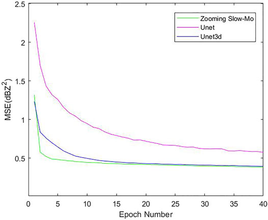
FIGURE 7. Loss function curve of three different deep learning methods.

Furthermore, the performance results shown in Table 1 are obtained by testing on the test dataset. The MSE (total) refers to the mean square error index of the whole output. MSE (t2) refers to the mean square error index of the reflectivity data of the intermediate time point (with spatiotemporal downscaling at the same time). MSE (t1+t3) refers to the mean square error of reflectivity data at both time points (spatial downscaling only). From the indicator results, it can be seen that the deep learning method has a significant performance improvement compared with the traditional trilinear interpolation. In the deep learning methods, the Zooming Slow-Mo network exceeds UNet and UNet3D in various indicators, especially in the problem of temporal downscaling.

TABLE 1

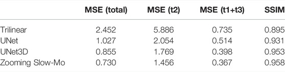
TABLE 1. Test set evaluation indicator.

To compare the actual downscaling effect, we plotted the downscaling radar reflectance images (Figure 8) and the difference between the reflectance images predicted by the downscaling algorithm and the true high-resolution image (Figure 9). First of all, according to the difference image effects shown in Figure 8, it can be found that the performance of the three deep learning downscaling algorithms provided in this study is much better than the traditional trilinear interpolation method. Furthermore, it can be found that when t1 and t3 generate downscaling images, three networks have obtained good results in the spatial downscaling data reconstruction effect because of the provision of raw low-resolution data. It can be found from Figure 9 that the colored scatter points of the Zooming Slow-Mo network in the interpolated image are sparse compared with Unet and UNet3D. Therefore, in the spatial downscaling task, the results obtained by Zooming Slow-Mo are closer to the real data effect. The time downscaling of t2 does not provide the original low-resolution data, so the prediction results obtained lack edge details compared with t1 and t3. However, according to Figure 8, it can be found that Zooming Slow-Mo is richer in shape details on the edge of data color stratification than the image drawn by UNet3D. It indicates that the generated data results will be more likely to obtain the simulated image high-resolution results for the complexity of the structure of the neural network and the diversification of operation behavior. The difference image of t2 data in Figure 9 indicates that the data scatter obtained by the Zooming Slow-Mo network is sparser than the first two networks. Therefore, the prediction results obtained by Zooming Slow-Mo are better than those of UNet and UNet3D in the spatiotemporal downscaling task. This situation shows that convolution LSTM seems a better solution to deal with temporal downscaling than convolution in the UNet series network. The mechanism of LSTM for processing timing information allows Zooming Slow-Mo extract information better which makes a faster convergence for the model.

FIGURE 8

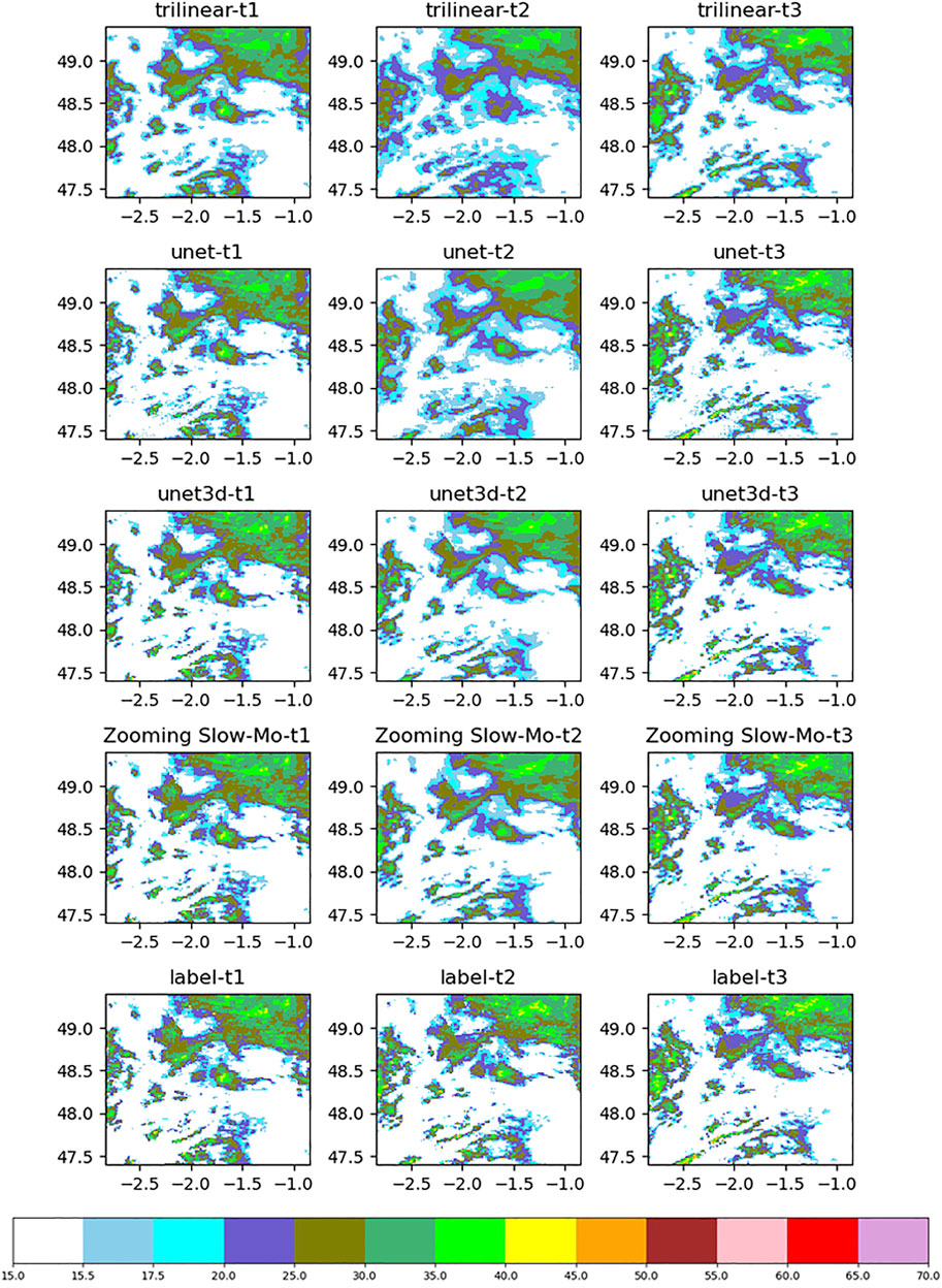
FIGURE 8. Precipitation reflectance image.

FIGURE 9

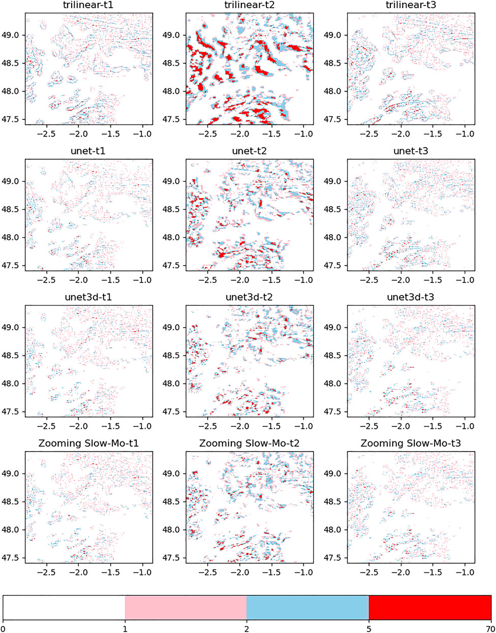
FIGURE 9. Image of the difference between the prediction and the real situation.

Data Fusion Performance Analysis

In this section, we tested a model separately with static data added alone (Zooming Slow-Mo-S), a model with static–dynamic data added alone (Zooming Slow-Mo-D), and the complete improved structure (Zooming Slow-Mo-DS), respectively. Finally, we got the loss function curve, as shown in Figure 10. As is seen from this figure, Zooming Slow-Mo has a stable curve and got the highest loss. Zooming Slow-Mo-D has a wave curve and the second highest loss. Zooming Slow-Mo-S and Zooming Slow-Mo-DS have a similar final loss which is the minimum value, but the former seems to have a curve that goes down faster than the latter. These phenomena indicate that Zooming Slow-Mo-S helps loss fall more smoothly and Zooming Slow-Mo-D makes the loss fall more unstably. In this experiment, the addition of static data performs better than the addition of dynamic data. However, there was no significant performance improvement in Zooming Slow-Mo-DS in the training process. It means that there is still room for improvement in the fusion of multiple types of data.

FIGURE 10

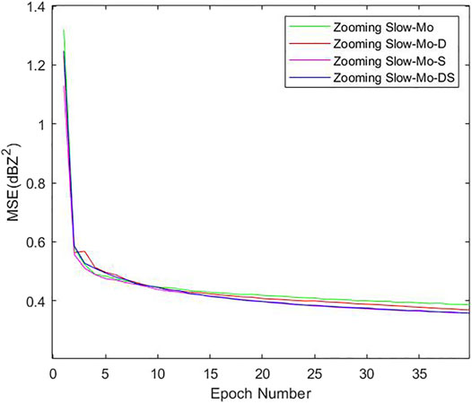
FIGURE 10. Loss function curve.

Further, the performance results shown in Table 2 are obtained by testing on the test dataset. From the MSE (total) indicator, Zooming Slow-Mo-DS got the best result, Zooming Slow-Mo-S became the second, and Zooming Slow-Mo-D became the third. It means that despite adding static data or dynamic data, the indicators will be improved. The method of using static data to affect the convolution position offset of the feature map got a better performance improvement. But the performance gain was not noticeable when the two improvement methods were combined. From the MSE (t2) indicator, Zooming Slow-Mo-DS still got the best result, Zooming Slow-Mo-S became the second, and Zooming Slow-Mo-D became the third. It showed that adding dynamic data to Zooming Slow-Mo-S will make the performance of the network better in temporal downscaling problems. From the MSE (t1+t3) indicator, it makes some difference; Zooming Slow-Mo-S got the best result, Zooming Slow-Mo-DS became the second, and Zooming Slow-Mo-D became the third. It indicates that adding dynamic data to Zooming Slow-Mo-S will make the performance of the network worse in spatial downscaling problems. From the SSIM indicator, three kinds of improvements got the same effect.

TABLE 2

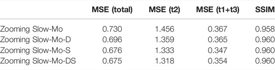
TABLE 2. Test set evaluation indicator.

The images of reflectivity and difference plotted in Figures 11, 12 are then analyzed. In the spatial downscaling of t1 and t3, the effect of the image is similar because the index improvement is not very obvious. The temporal and spatial downscaling of t2 is different. According to the generated reflectivity image, it can be found that the addition of dynamic data will inhibit the filling of high-frequency data. From the prediction results of t2, it can be found that Zooming Slow-Mo-S can better recover the data between the 45-dB and 50-dB range in the upper half of the data. The data processing effect of Zooming Slow-Mo-DS in the range of 30dB–40dB is weaker than Zooming Slow-Mo-S and Zooming Slow-Mo-D. Furthermore, it can still be found from the difference image that the amount of large difference data generated by Zooming Slow-Mo-DS is relatively less. Overall, the image effect obtained by Zooming Slow-Mo-S is more in line with the real situation.

FIGURE 11

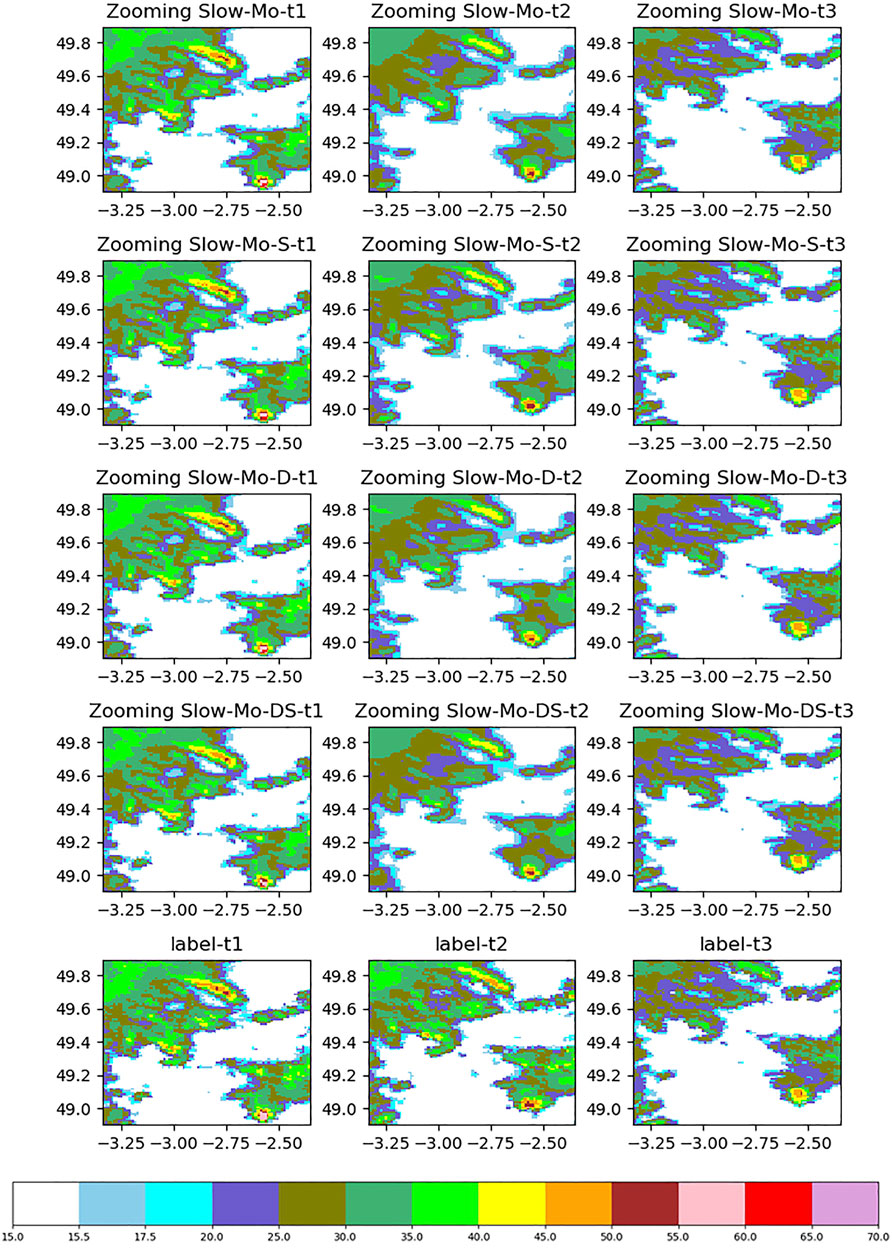
FIGURE 11. Precipitation reflectance image.

FIGURE 12

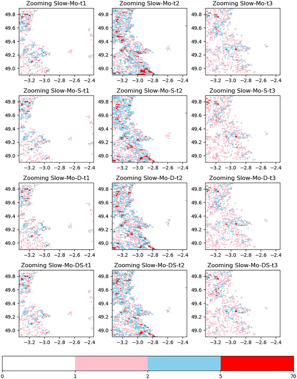
FIGURE 12. Image of the difference between the prediction and the real situation.

These results verify that the strategy of fusion works. With the help of deformable convolution, static data can make a greater position rule than the rule which is affected by dynamic data alone. It means that static data are more fit for dealing with affecting inherent rules. Dynamic data can also affect the model, but the effect is extremely weak. It is obvious that the feature fusion method based on splicing has little effect. The problem of how to use dynamic data efficiently is still worth thinking.

Conclusion

In this work, we studied the applicability of deep learning in spatial and temporal downscaling problems. Therefore, we mainly focused on the radar precipitation reflectivity data. At the same time, trilinear interpolation, UNet, UNet3D, and one-stage Zooming Slow-Mo network structures are selected for data testing. According to the data results, Zooming Slow-Mo can get better results. Furthermore, we have made appropriate improvements for Zooming Slow-Mo: one method is to use static data to affect the position offset features of deformable convolution, and the other way is to use dynamic data as input to affect convolution mapping. These two methods improve the training indicators, while the former is relatively better. In the end, we combined the two improvements, although Zooming Slow-Mo-DS has a slight improvement in the data on the indicator relative to Zooming Slow-Mo-S, and the actual output of the image effect is not as good as Zooming Slow-Mo-S.

To verify these conclusions, we drew each network’s training curve, as shown in Figures 7, 10. We provided the test indexes of each network under the test set, as shown in Tables 1, 2. Furthermore, we drew heat graphs and difference graphs of actual precipitation reflectance; the heat graphs are shown in Figures 8, 11 and the difference graphs are shown in Figures 9, 12. From the training curves, we found that the Zooming Slow-Mo network exceeds UNet and UNet3D in various indicators, especially in the problem of temporal downscaling. The addition of static data performs better than the addition of dynamic data on the convergence of the loss function. From the test indexes, we can find that deep learning methods outperform trilinear interpolation by a wide margin. In addition, Zooming Slow-Mo gets the best performance because of deformable convolution and LSTM. The addition of dynamic and static data enables the network to obtain varying performance benefits. Finally, from the heat graphs and difference graphs, we observed a real downscaling image effect. Because of this, we get the view that the problem of how to use dynamic data efficiently is still worth thinking about.

To verify the authenticity of performance improvement, we compared the results with the DCN network (Serifi et al., 2021). The author of DCN also carried out downscaling in rainfall, but the unit of the source data is $g/m^2$. In our work, the unit is based on the reflectivity which is called $dBZ$. These two units are both common units, and they can be converted under the condition that we know some local constants. Without compromising the reliability of the values, we decided to compare the reduction indicator. The author of DCN chose trilinear interpolation as the baseline and calculated the decrease rate of the MSE index. The decrease rate is the reduction indicator. The indicator of DCN and other networks in our experiment are shown in Table 3.

TABLE 3

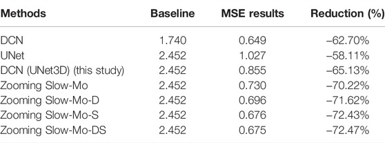
TABLE 3. Performance comparison with DCN.

As we can see from Table 3, the DCN got a reduction of −62.70%. We tested the same network in our dataset, and it got a reduction of −65.13%. It means that the DCN really gets improvements, and it can be applied to different datasets. But Zooming Slow-Mo seems great, and it got a 5% performance improvement. With the help of stable and dynamic data, it can even get more performance improvement.

It is worth mentioning that Zooming Slow-Mo can also be adapted to other meteorological elements. Elements like snowfall and rainfall can be directly adapted because they have a transformation of high-frequency information and fast change rate. However, elements like air pressure and temperature cannot be adapted. These elements have more low-frequency information and a slower rate of change. In some articles, authors prefer to use residual convolution to handle elements like temperature and remove residual convolution to handle elements like rainfall. These strategies truly make sense. Therefore, before dealing with elements like temperature, we still need to add more residual convolution as a strategy. Furthermore, the dynamic data which are used to affect the original data should also be considered. These plans will be further tested and improved in our subsequent experiments.

To solve the downscaling problem by deep learning, the work we have carried out is only the basic part of the algorithm test. There are still many problems that need to be studied on this basis.

1) As an unexplainable model, deep learning makes the low-resolution data reconstructed into high-resolution data in a data-driven way, and this method lacks the constraints of physical factors. Therefore, the appropriate use of dynamic models (such as adding regularization factors to the loss function and improving the weight update strategy) will be a promising performance optimization scheme (Chen et al., 2020).

2) The study we have completed is only the basic algorithm function of the downscaling of precipitation reflectance elements. In the actual situation, the function needs to be applied to different tasks or different areas, and it is known that meteorological observations vary from year to year due to climate change. In view of the way of using a single model to adapt to a variety of situations cannot get good test results, we believed that each meteorological element or each regional scope needs a separate network or unique weight to test necessarily. Therefore, using a deep learning network to solve the scaling problem needs to build a complete network selection system. It is necessary for the system to configure the latest data in real time to update the model weight and prepare a special model weight for a special environment.

3) The deep learning network in this study is only suitable for a regular meteorological element grid. However, the unstructured or irregular network topology is the more real state of meteorological data (Kipf and Welling, 2016; Qi et al., 2017). Therefore, the downscaling solution for any grid topology is worth studying.

Data Availability Statement

The Dataset is licenced by METEO FRANCE under Etalab Open Licence 2.0. Reuse of the dataset is free, subject to an acknowledgement of authorship. For example: METEO FRANCE - Original data downloaded from https://meteonet.umr-cnrm.fr/, updated on 30 January 2020.

Author Contributions

HQ: project administration, funding acquisition, supervision, and writing—review and editing. YD: conceptualization. HC: methodology, data curation, validation, visualization, and writing—original draft.

Conflict of Interest

The authors declare that the research was conducted in the absence of any commercial or financial relationships that could be construed as a potential conflict of interest.

The reviewer JC declared a shared affiliation with the authors to the handling editor at the time of review.

Publisher’s Note

All claims expressed in this article are solely those of the authors and do not necessarily represent those of their affiliated organizations, or those of the publisher, the editors, and the reviewers. Any product that may be evaluated in this article, or claim that may be made by its manufacturer, is not guaranteed or endorsed by the publisher.

References

Accarino, G., Chiarelli, M., Immorlano, F., Aloisi, V., Gatto, A., and Aloisio, G. (2021). MSG-GAN-SD: A Multi-Scale Gradients GAN for Statistical Downscaling of 2-Meter Temperature over the EURO-CORDEX Domain. Ai 2, 600–620. doi:10.3390/ai2040036

CrossRef Full Text | Google Scholar

Adewoyin, R. A., Dueben, P., Watson, P., He, Y., and Dutta, R. (2021). TRU-NET: a Deep Learning Approach to High Resolution Prediction of Rainfall. Mach. Learn 110, 2035–2062. doi:10.1007/s10994-021-06022-6

CrossRef Full Text | Google Scholar

Beck, H. E., Pan, M., Roy, T., Weedon, G. P., Pappenberger, F., van Dijk, A. I. J. M., et al. (2019). Daily Evaluation of 26 Precipitation Datasets Using Stage-IV Gauge-Radar Data for the CONUS. Hydrol. Earth Syst. Sci. 23, 207–224. doi:10.5194/hess-23-207-2019

CrossRef Full Text | Google Scholar

Berg, P., Moseley, C., and Haerter, J. O. (2013). Strong Increase in Convective Precipitation in Response to Higher Temperatures. Nat. Geosci. 6, 181–185. doi:10.1038/ngeo1731

CrossRef Full Text | Google Scholar

Ceccherini, G., Ameztoy, I., Hernández, C., and Moreno, C. (2015). High-resolution Precipitation Datasets in South America and West Africa Based on Satellite-Derived Rainfall, Enhanced Vegetation Index and Digital Elevation Model. Remote Sens. 7, 6454–6488. doi:10.3390/rs70506454

CrossRef Full Text | Google Scholar

Chen, X., Feng, K., Liu, N., Lu, Y., Tong, Z., Ni, B., et al. (2020). RainNet: A Large-Scale Dataset for Spatial Precipitation Downscaling.

Google Scholar

Dai, J., Qi, H., Xiong, Y., Li, Y., Zhang, G., Hu, H., et al. (2017). “Deformable Convolutional Networks,” in Proceedings of the IEEE international conference on computer vision), 764–773.

CrossRef Full Text | Google Scholar

Höhlein, K., Kern, M., Hewson, T., and Westermann, R. J. M. A. (2020). A Comparative Study of Convolutional Neural Network Models for Wind Field Downscaling. 27, e1961.doi:10.1002/met.1961

CrossRef Full Text | Google Scholar

Han, J., Wang, C. J. I. T. O. V., and Graphics, C. (2020). SSR-TVD: Spatial Super-resolution for Time-Varying Data Analysis and Visualization.doi:10.1109/tvcg.2020.3032123

CrossRef Full Text | Google Scholar

Kingma, D. P., and Ba, J. J. a. P. A. (2014). Adam: A Method for Stochastic Optimization.

Google Scholar

Kipf, T. N., and Welling, M. J. a. P. A. (2016). Semi-supervised Classification with Graph Convolutional Networks.

Google Scholar

Lanza, L. G., Ramírez, J., Todini, E. J. H., and Sciences, E. S. (2001). Stochastic Rainfall Interpolation and Downscaling. Hydrology Earth Syst. Sci. 5, 139–143.

CrossRef Full Text | Google Scholar

Larvor, G., Berthomier, L., Chabot, V., Le Pape, B., Pradel, B., and Perez, L. (2020). MeteoNet, An Open Reference Weather Dataset by METEO FRANCE.

Google Scholar

Lee, D., Lee, S., Lee, H. S., Lee, H.-J., and Lee, K. (2019). “Context-preserving Filter Reorganization for VDSR-Based Super-resolution,” in 2019 IEEE International Conference on Artificial Intelligence Circuits and Systems (AICAS) (IEEE), 107–111.

CrossRef Full Text | Google Scholar

Lee, T., and Jeong, C. (2014). Nonparametric Statistical Temporal Downscaling of Daily Precipitation to Hourly Precipitation and Implications for Climate Change Scenarios. J. Hydrology 510, 182–196. doi:10.1016/j.jhydrol.2013.12.027

CrossRef Full Text | Google Scholar

Lu, Z., Chen, Y. J. S., Image, , and Processing, V. (2021). Single Image Super-resolution Based on a Modified U-Net with Mixed Gradient Loss, 1–9.

Google Scholar

Mao, X., Shen, C., and Yang, Y.-B. J. a. I. N. I. P. S. (2016). Image Restoration Using Very Deep Convolutional Encoder-Decoder Networks with Symmetric Skip Connections. 29, 2802–2810.

Google Scholar

Maraun, D., Wetterhall, F., Ireson, A., Chandler, R., Kendon, E., Widmann, M., et al. (2010). Precipitation Downscaling under Climate Change: Recent Developments to Bridge the Gap between Dynamical Models and the End User. 48.doi:10.1029/2009rg000314

CrossRef Full Text | Google Scholar

Monjo, R. (2016). Measure of Rainfall Time Structure Using the Dimensionless N-Index. Clim. Res. 67, 71–86. doi:10.3354/cr01359

CrossRef Full Text | Google Scholar

Pan, B., Hsu, K., Aghakouchak, A., and Sorooshian, S. (2019). Improving Precipitation Estimation Using Convolutional Neural Network. Water Resour. Res. 55, 2301–2321. doi:10.1029/2018wr024090

CrossRef Full Text | Google Scholar

Prein, A. F., Langhans, W., Fosser, G., Ferrone, A., Ban, N., Goergen, K., et al. (2015). A Review on Regional Convection‐permitting Climate Modeling: Demonstrations, Prospects, and Challenges. Rev. Geophys. 53, 323–361. doi:10.1002/2014rg000475

PubMed Abstract | CrossRef Full Text | Google Scholar

Qi, C. R., Yi, L., Su, H., and Guibas, L. J. J. a. P. A. (2017). Pointnet++: Deep Hierarchical Feature Learning on Point Sets in a Metric Space.

Google Scholar

Rodrigues, E. R., Oliveira, I., Cunha, R., and Netto, M. (2018). “DeepDownscale: a Deep Learning Strategy for High-Resolution Weather Forecast,” in 2018 IEEE 14th International Conference on e-Science (e-Science) (IEEE), 415–422. doi:10.1109/escience.2018.00130

CrossRef Full Text | Google Scholar

Ronneberger, O., Fischer, P., and Brox, T. (2015). “U-net: Convolutional Networks for Biomedical Image Segmentation,” in International Conference on Medical image computing and computer-assisted intervention (Springer), 234–241.

CrossRef Full Text | Google Scholar

Sahour, H., Sultan, M., Vazifedan, M., Abdelmohsen, K., Karki, S., Yellich, J., et al. (2020). Statistical Applications to Downscale GRACE-Derived Terrestrial Water Storage Data and to Fill Temporal Gaps. Remote Sens. 12, 533. doi:10.3390/rs12030533

CrossRef Full Text | Google Scholar

Serifi, A., Günther, T., and Ban, N. J. F. I. C. (2021). Spatio-Temporal Downscaling of Climate Data Using Convolutional and Error-Predicting Neural Networks. 3, 26.doi:10.3389/fclim.2021.656479

CrossRef Full Text | Google Scholar

Sha, Y., Gagne Ii, D. J., West, G., Stull, R., and Climatology, (2020). Deep-Learning-Based Gridded Downscaling of Surface Meteorological Variables in Complex Terrain. Part II: Daily Precipitation. Part II Dly. Precip. 59, 2075–2092. doi:10.1175/jamc-d-20-0058.1

CrossRef Full Text | Google Scholar

Shi, W., Caballero, J., Huszár, F., Totz, J., Aitken, A. P., Bishop, R., et al. (2016). “"Real-time Single Image and Video Super-resolution Using an Efficient Sub-pixel Convolutional Neural Network,” in Proceedings of the IEEE conference on computer vision and pattern recognition), 1874–1883.

CrossRef Full Text | Google Scholar

Stengel, K., Glaws, A., Hettinger, D., and King, R. N. (2020). Adversarial Super-resolution of Climatological Wind and Solar Data. Proc. Natl. Acad. Sci. U.S.A. 117, 16805–16815. doi:10.1073/pnas.1918964117

PubMed Abstract | CrossRef Full Text | Google Scholar

Sun, D., Wu, J., Huang, H., Wang, R., Liang, F., and Xinhua, H. J. M. P. I. E. (2021). Prediction of Short-Time Rainfall Based on Deep Learning, 2021.

CrossRef Full Text | Google Scholar

Tran Anh, D., Van, S. P., Dang, T. D., and Hoang, L. P. (2019). Downscaling Rainfall Using Deep Learning Long Short‐term Memory and Feedforward Neural Network. Int. J. Climatol. 39, 4170–4188. doi:10.1002/joc.6066

CrossRef Full Text | Google Scholar

Vandal, T., Kodra, E., Ganguly, S., Michaelis, A., Nemani, R., and Ganguly, A. R. (2017). “Deepsd: Generating High Resolution Climate Change Projections through Single Image Super-resolution,” in Proceedings of the 23rd acm sigkdd international conference on knowledge discovery and data mining), 1663–1672.

Google Scholar

Wang, Y., Perazzi, F., Mcwilliams, B., Sorkine-Hornung, A., Sorkine-Hornung, O., and Schroers, C. (2018). “A Fully Progressive Approach to Single-Image Super-resolution,” in Proceedings of the IEEE conference on computer vision and pattern recognition workshops), 864–873.

CrossRef Full Text | Google Scholar

Ward, C. M., Harguess, J., Crabb, B., and Parameswaran, S. (2017). “Image Quality Assessment for Determining Efficacy and Limitations of Super-resolution Convolutional Neural Network (SRCNN),” in Applications of Digital Image Processing XL (International Society for Optics and Photonics), 1039605.

CrossRef Full Text | Google Scholar

Wasko, C., and Sharma, A. J. N. G. (2015). Steeper Temporal Distribution of Rain Intensity at Higher Temperatures within Australian Storms.

Google Scholar

Xiang, X., Tian, Y., Zhang, Y., Fu, Y., Allebach, J. P., and Xu, C. (2020). “Zooming Slow-Mo: Fast and Accurate One-Stage Space-Time Video Super-resolution,” in Proceedings of the IEEE/CVF conference on computer vision and pattern recognition), 3370–3379.

CrossRef Full Text | Google Scholar

Xingjian, S., Chen, Z., Wang, H., Yeung, D.-Y., Wong, W.-K., and Woo, W.-C. (2015). “Convolutional LSTM Network: A Machine Learning Approach for Precipitation Nowcasting,” in Advances in neural information processing systems), 802–810.

Google Scholar

Yao, L., Wei, W., and Chen, L. (2016). How Does Imperviousness Impact the Urban Rainfall-Runoff Process under Various Storm Cases? Ecol. Indic. 60, 893–905. doi:10.1016/j.ecolind.2015.08.041

CrossRef Full Text | Google Scholar

Zhang, J., and Huang, D. (2019). “Image Super-resolution Reconstruction Algorithm Based on FSRCNN and Residual Network,” in 2019 IEEE 4th International Conference on Image, Vision and Computing (ICIVC) (IEEE), 241–246. doi:10.1109/icivc47709.2019.8981280

CrossRef Full Text | Google Scholar