Volcanic and Seismic Source Modeling: An Open Tool for Geodetic Data Modeling

Highlights

- Volcanic and seismic source modeling (VSM) is a Python tool to model geodetic data

- VSM supports deformation data detected by satellite and terrestrial techniques

- VSM performs data inversion by global optimization or Bayesian inference

- VSM can be used for near real-time applications and high-level scientific research

- VSM is open-source. Code, GUI, and notebooks are freely available at github.com/EliTras/VSM

1 Introduction

Natural processes and anthropogenic activities often generate changes in the stress state of the crust and, consequently, measurable surface deformation. Natural processes such as volcanic activity produce surface displacements due to many phenomena, including magma recharge/deployment and migration, fluid flow, and other internal processes related to magma crystallization and degassing. Volcano geodesy is crucial to define the state of volcanoes (Poland and de Zeeuw-van Dalfsen, 2021) and for eruptive hazard assessment (Sparks et al., 2012; Biggs et al., 2014). The accurate measurement of surface deformation is one of the most relevant parameters to estimate tectonic stress accumulation and release (DeMets et al., 1990) for studying the seismic cycle (Wright et al., 2004; Weston et al., 2011) and the intraplate coupling (Hashimoto et al., 2009). Improved monitoring capabilities also capture surface deformations related to coastal erosion and its connection to climate change (Shirzaei and Bürgmann, 2018), slope failures, landslides, and deep-seated gravitational slopes (Colesanti and Wasowski, 2006; Saroli et al., 2021) and other hydrogeological disasters (Galloway and Hoffmann, 2007). In addition, anthropogenic activity such as mining and water pumping causes measurable ground displacement (Chen et al., 2020).

Earth’s surface deformations are measured by means of remote sensing and terrestrial techniques, reaching sub-millimeter accuracy. Synthetic Aperture Radar (SAR) satellites have been quickly developing in the last decades in terms of cost lowering, improvement of processing algorithms, and (near) real-time data availability (Biggs and Wright, 2020). European Space Agency’s (ESA) satellites Sentinel 1A-B provide open-access data for the whole solid Earth surface every 6 or 12 days. Interferometric SAR (InSAR) analysis produces high-quality, coherent data covering wide areas along the satellite’s Line of Sight (LOS). GNSS data allow mapping of nearly 3D deformation patterns, but often the network consists of few benchmarks. Leveling is a branch of classic surveying that measures the orthometric height difference between the benchmarks of a network. It is used to measure the vertical displacement with high accuracy. Electronic Distance Measurement (EDM) is another terrestrial technique measuring the distance between two benchmarks through electromagnetic waves. Borehole observations such as dilatometers provide measurements of the volumetric strain (i.e., the unit change in volume), whereas tiltmeters record the inclination to the vertical or horizontal (Agnew, 1986). Tilt and strain can detect the slightest change of the deformation field amounting to parts per million (ppm).

Theoretical models of deformation sources are commonly employed to investigate the surface displacements observed, for example, in volcanic areas or related to a seismic event (Segall, 2010). A volcanic source can be represented by a confined part of crust with a certain shape (e.g., sphere, spheroid, and penny-shaped crack) inflating/deflating because of a change in the internal magma/gas pressure (Figure 1). Similarly, the static seismic source is ideally represented by a tabular discontinuity in the crust undergoing relative movement on both sides. Furthermore, deformations of anthropogenic and natural—not geophysical—origins, such as gas reservoir exploitation, water pumping, and soil consolidation, can be represented using the same models. Analytical deformation models usually approximate the local crust as homogeneous and isotropic half-spaces. Catalogs of the most common analytical deformation models are presented by Lisowski (2007) and Battaglia et al. (2013b). The source models shown in Figure 1 provide different boundary conditions for the elastic equations in the medium and therefore lead to surface displacement fields that differ in terms of pattern, spatial extension, and gradient. Moreover, the ratio between vertical and horizontal maximum displacement components varies. Because the specific surface pattern can be considered a signature of the model itself, in theory, it is possible to choose the most appropriate deformation source based on the observed deformation. With real data, this choice carries a high level of epistemic uncertainty, depending on the resolving power of geodetic ground networks and satellite coverage. Furthermore, the limitations of assuming the crust as a flat, isotropic, homogeneous, and elastic half-space are well known (Trasatti et al., 2003; Masterlark, 2007 and references therein). Regardless, analytical models of deformation sources still provide a rapid, powerful, and computationally cheap method to estimate significant parameters—at least of first order—related to volcanic and seismic activity from monitoring data.

FIGURE 1

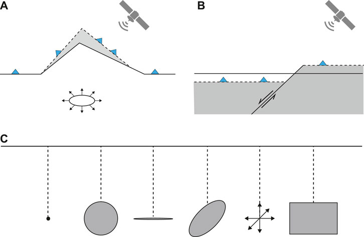
FIGURE 1. Formulation of the non-linear inverse problem of ground deformations due to volcanic and seismic sources. (A) A change in the conditions in the deep reservoir causes a variation in the distribution of stress in the local crust and surface deformation. (B) Similarly, the sudden slip on the seismic fault during an earthquake causes permanent deformation. The ground deformation is detectable by geodetic surveys (in situ, blue triangles and remote sensing). (C) It is possible to model the observed data using a theoretical representation of the volcanic or seismic source. The inversion procedure is aimed at retrieving the parameters of the model implemented. The forward models available in VSM are, from left to right, isotropic point-source (Mogi, 1958), finite volume sphere (McTigue, 1987), penny-shaped crack (Fialko et al., 2001), arbitrarily oriented prolate spheroid (Yang et al., 1988), moment tensor point-source (Davis, 1986), and rectangular dislocation (Okada, 1985).

Geodetic data inversions are commonly performed to constrain source parameters and their associated uncertainties. Several geodetic inversion packages have been developed and published in the last years (Battaglia et al., 2013a; Bagnardi and Hooper, 2018; Cannavò, 2019). They are all MATLAB^® based and differ in terms of the forward models and their possible combination, considered datasets, or adopted non-linear inversion method. In particular, dModels (Battaglia et al., 2013a) provides functions to model sources among sphere, spheroid, penny-shaped crack, and rectangular dislocation, using a dataset from InSAR, GNSS, tilt, and strain data. GBIS (Bagnardi and Hooper, 2018) implements a Bayesian approach for the inversion of InSAR and GNSS data using, among others, analytical routines from dModels. GAME (Cannavò, 2019) provides a user interface. Because it is designed for station-based measurements, besides GNSS data, it supports EDM data but not InSAR. Modeling of volcanic and seismic sources is included in the interferometric module of the commercial software for SAR data processing SARscape^® (SARmap). It supports various SAR products (e.g., LOS and offset tracking) and GNSS data. Finally, Pyrocko (Heimann et al., 2019) is a Python framework designed for seismic source problems. Among others, it performs modeling of InSAR, GNSS data, and dynamic waveforms. As the most common volumetric sources are not supported, application to volcanic areas is not straightforward (e.g., BEAT for Bayesian parameters estimation of Okada-like and moment tensor sources, Vasyura-Bathke et al., 2020). Furthermore, the KITE toolkit from Pyrocko can be used for InSAR post-processing.

This study presents the open-source Python tool Volcanic and Seismic source Modeling (VSM) in all its components. This software package collects the most common and versatile analytical sources as the forward models and supports remote sensing and terrestrial geodetic datasets, single or in combination. The present version of VSM has been tested in all its modules against the original and stable Fortran code (executable in Trasatti, 2019) and has been incrementally updated with 1) a second sampling algorithm, 2) additional forward models, 3) many data categories supported, 4) a Graphical User Interface (GUI), 5) Jupyter Notebook technology and several other aspects. VSM implements two sampling algorithms: a global optimization algorithm based on Voronoi tessellation of the parameter space and a probabilistic approach to parameters estimation based on the Bayes theorem. The tool runs from Python script, GUI, and Jupyter Notebooks. It is freely available at https://github.com/EliTras/VSM. With respect to the software mentioned above, VSM is the only one designed with a portfolio of analytical models (single or in combination), data from the most common geodetic techniques (single dataset or in combination with weights), two different sampling algorithms for cross-checking, and completely open with large portability. The open-access and modular structure of VSM allows for diffusion and personalization with, for example, additional data types and forward models. Its broad applications range from high-level research to teaching and from single studies to near real-time hazard estimates. Potential users range from early-career scientists to experts. This study presents the functionalities of VSM and its practical use. The last sections are dedicated to applying to the 2011–2013 unrest at Campi Flegrei caldera (Italy), with comparisons among 22 tests using different settings, freely available at https://github.com/EliTras/VSM_test.

2 VSM Functionalities

VSM is designed to estimate source parameters of the most common analytical sources of deformation by using geodetic data (Figure 1). It is structured as a typical overdetermined non-linear inverse problem (Tarantola, 1987), in which data are known whereas the parameters of the source(s) that generated the observed data are unknown. The scheme of VSM is reported in Figure 2. The first block is the VSM input, consisting of the collection of geodetic observations, the selection of one or more deformation sources as the forward model (with a related search range for each parameter), and the selection of the sampling algorithm (with a few setting parameters). The data inversion block is the VSM execution based on the chosen algorithm. The last block is the VSM output. It consists of several products such as the sampled parameter space, the parameters distributions, the optimal parameters, and synthetic data. Each part of the scheme in Figure 2 is discussed in the following sections.

FIGURE 2

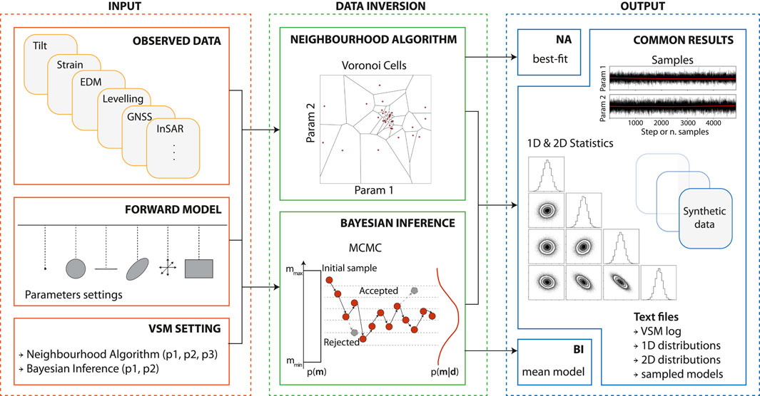
FIGURE 2. Scheme of the VSM. The input of VSM consists of at least one dataset. The forward model is one or more analytical sources among those reported in Figure 1. One of the two available sampling algorithms can be selected. Several products are generated as output.

2.1 Data Input

VSM supports the following types of data: InSAR (may include multiple files from different sensors and/or orbits), GNSS, leveling, EDM, tilt, and strain. Data units can be either displacements (measured in meters) or mean velocities (if annual rates, m/yr). The parameters related to the source intensity (discussed in Section 2.2) are measured accordingly (i.e., if the input data are expressed in meters, the resulting estimation of volume variation is expressed in cubic meters, and if the input data are m/yr, the volume variation is the annual rate is m³/yr). Tilt and strain are non-dimensional, and the units are microradians and microstrains (ppm or 10⁻⁶), respectively. The layout of the data files accepted by VSM is shown in Table 1. VSM supports the following data formats—plain text, comma-separated values files (both with or without header), and ESRI^® Shapefiles—which are automatically identified by the system.

TABLE 1

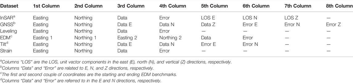
TABLE 1. Structure of the supported data files. “Easting” and “northing” are the geographical coordinates projected in meters.

InSAR results typically consist of hundreds of thousands of points. This type of data should be pre-processed with downsampling algorithms. The treatment of InSAR data has a non-negligible impact on the balance among keeping the features of the deformation, maintaining the resolving power of the source parameters, and being computationally affordable at the same time. The general indication is to achieve denser sampling in near-field regions and coarser at a greater distance. More sophisticated downsampling techniques based on InSAR covariance have been developed (Lohman and Simons, 2005). The LOS unit vector components must be specified at each data point (Table 1) and can be computed considering variable radar incidence ϑ and heading ϕ angles:

$LOS E=-\sin \vartheta \cos \varphi ; LOS N=\sin \vartheta \sin \varphi ;LOSZ=\cos \vartheta ,$

where E, N, and Z are the east, north, and vertical components. For most SAR sensors, ϑ ranges from 23° to more than 40° from the vertical, whereas ϕ is around −10°/−15° for ascending satellite passes (flight direction NNW) and around −165°/−170° for descending passes (flight direction SSW). The combination of multiple InSAR datasets with different imaging geometries helps overcome the limitation of the radar single look. Moreover, using other techniques such as offset tracking allows estimating displacements in the azimuth direction, in addition to the slant range. Datasets derived from these techniques are all accepted by VSM by providing suitable unit vectors accompanying the data.

In the case of multiple datasets from different techniques, a joint inversion can be performed. In this case, weights for each dataset should be assigned by the user. The weight can be any decimal or integer number. Otherwise, it is considered equal to 1 if the related dataset is supplied without a specified weight or 0 if that data type is not present. In any case, all weights provided are scaled to 1 in total because VSM considers the relative weight of each dataset. In the case of multiple InSAR datasets, they are accounted for with a single weight. In this case, the relative weight among different satellites and/or orbits is given by the balance between the number of data points and the uncertainty associated with each InSAR dataset. The weights among data from different techniques are somehow arbitrary and combine with the number of data points and with the relative signal-to-noise ratio of each dataset. Weights can be chosen after several tests, checking the trend of improvement/worsening of the misfit of each dataset and the total one (Trasatti et al., 2015).

2.2 Forward Model

The forward analytical models available in VSM are listed in Figure 1, whereas their free parameters are shown in Table 2. For all these models, the medium is an isotropic, homogeneous, and elastic half-space.

TABLE 2

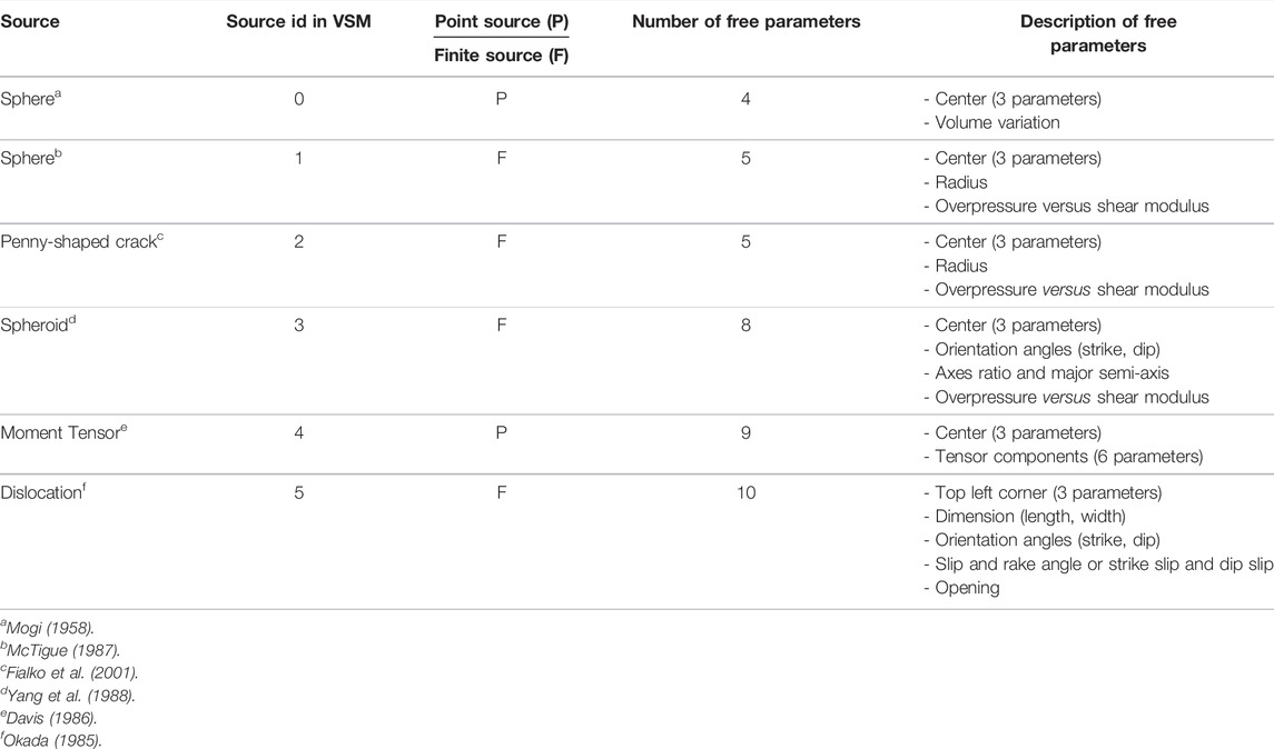
TABLE 2. Forward analytical sources available in VSM and their associated free parameters.

The simplest model to represent the expansion of a magma chamber at depth is a point dilatation source, which is considered a fair approximation of a spherical overpressure source (Mogi, 1958). Approximate analytical solutions for a finite volume sphere were developed by McTigue (1987), useful when the depth is comparable with the source radius. The prolate spheroid is a cavity with a 3D orientation in the half-space (Yang et al., 1988), usually employed to represent vertically or along-dip elongated batches of magma uprising in the crust besides pressurized reservoirs. While the spherical source represents axisymmetric extended reservoirs, spheroidal volumes are more versatile and may approximate magma bodies and conduits with arbitrary orientation. The most common model for deformation due to earthquakes or aseismic slip is the “Okada” model (Okada, 1985). It provides static elastic solutions due to constant slip applied on a rectangular dislocation. It may also represent sill-like tabular reservoirs, dikes, and hydro-fractures with thickness much smaller than the other dimensions. Similarly, the penny-shaped crack (Fialko et al., 2001) is a model for horizontal sills and hydro-fractures. A further and very general category of deformation models is described in terms of the combination of forces. The moment tensor source is a point source composed of dipoles and double couples and implicitly defines a large variety of sources (Mindlin, 1936; Eshelby, 1957; Davis, 1986). It may be used if the source shape is unknown, although its geometrical interpretation is not straightforward and not always unique (Trasatti et al., 2011; Amoruso and Crescentini, 2013). The first step for the interpretation is the diagonalization of the moment tensor. Based on the combination of the principal values of the moment tensor (the matrix eigenvalues), a subset of solutions may represent a sphere (if the principal moments are equal), a shear dislocation (the moment tensor is a double couple), an ellipsoid arbitrary oriented in space, all with point-source approximation (Davis, 1986; Trasatti et al., 2011). Therefore, from the ratios between the principal values of the moment tensor, it is possible to look at Table 1 by Davis (1986) or approach the formal analytical inversion to retrieve, if they exist, the ellipsoid axes ratios.

VSM requires the definition of the range of search of each parameter. The parameter is fixed a priori if the minimum and maximum are equal. Units are meters for spatial coordinates. Source intensity parameters are volume variation, overpressure versus shear modulus (ΔP/μ), tensor components, dislocation slip, and opening. They scale linearly with data and are expressed in units accordingly with data (absolute values or annual rates).

2.3 Data Inversion

VSM performs non-linear inversions and implements two different sampling algorithms that can be chosen by the user. The first is a global optimization algorithm based on the neighborhood algorithm (NA, Sambridge, 1999a), and the second follows a probabilistic approach to parameter estimation based on the Bayes theorem (here called Bayesian inference, BI). Several Python libraries for global optimization and Bayesian inference have been tested (e.g., SciPy Optimize and other packages from GitHub and PyPI), but as the number of unknowns or data points increases, the performance becomes unsatisfactory in terms of computational effort and sampling of the parameter space.

2.3.1 Neighborhood Algorithm

The NA is a derivative-free search method that uses Voronoi cells to sample the multi-dimensional parameter space (Sambridge, 1999a). The Voronoi cells are multi-dimensional regions in which the parameter space is subdivided (Voronoï, 1908; Figure 2). These convex polyhedral cells are defined as nearest neighbors under a predefined norm (usually l²-norm). The purpose is to find points (models) with acceptable values of the supplied objective function. A uniform random walk by a Gibbs sampler (Geman and Geman, 1984) is restricted to each Voronoi cell, while the conditional probability density function outside the cell is set to zero. Asymptotically, the samples produced by this walk will be uniformly distributed inside the cell regardless of its shape (Sambridge, 1999a). The direct search is basically independent of the initial sampling, self-adaptative, and driven by the models with the lowest objective function. Formerly implemented in receiver function studies to define the crustal seismic structure (Reading et al., 2003; Bianchi et al., 2008), the NA has been applied in other branches of geophysical non-linear inverse problems (Kennett et al., 2000; Snoke, 2002; Trasatti et al., 2015).

The objective function of the NA in VSM is the reduced chi-square, a l²-norm. For each set of parameters m, the synthetic surface displacements of the chosen forward model are computed d^syn(m). The objective function is defined as the measure of the discrepancy between observed data d and predictions d^syn as follows:

${\chi }_m^2=\frac{1}{N}{\displaystyle \sum \frac{{\left(d-d^{syn}\right)}^2}{{\sigma }^2}}(1)$

where σ is the uncertainty associated with data and N the number of data points of the given dataset. In the following, the data covariance matrix is considered diagonal, so it is assumed that the data points are independent and accompanied by their variance. Because more than one forward source can be considered, the total forward model d^syn(m) is the sum of the contribution of each source to the surface displacement field. In case of multiple data types, specific weights should be assigned (InSAR, w^sar; GNSS, w^gps; leveling, w^lev; EDM, w^edm; tilt, w^tlt; strain, w^srn) as discussed in Section 2.1. The objective function ${\chi }_m^2{}^{tot}$ accounting for each misfit and relative weight is

${\chi }_m^2{}^{tot}={\displaystyle \sum _{set}{w}^{set}{\chi }_m^2{}^{set}} (2)$

where ${\chi }_m^2{}^{set}$ is the objective function in Eq. 1 defined for each dataset and w^set the corresponding weight (set = sar, gps, lev, edm, tlt, srn). VSM also computes the null reduced chi-square of each dataset, corresponding to Eq. 1 in the hypothesis of d^syn = 0:

${\chi }_m^2{}^{null}=\frac{1}{N}{\displaystyle \sum {\left(\frac{d}{\sigma }\right)}^2}(3)$

${\chi }_m^2{}^{null}$ is a measure of the ratio between the signal and associated uncertainty, and it is indicative of the goodness of fit when Eq. 1 is calculated.

The NA requires a few parameters ruling the inversion: the number of samples (Voronoi cells) for each iteration (p1), the number of cells to be re-sampled among those providing the lowest misfit (p2), and the total number of iterations (p3). In VSM, the NA search module is taken from the PyPI package (https://pypi.org/project/neighborhood/). The NA original routine has been modified to manage parameters that are fixed a priori.

2.3.2 Bayesian Inference

The Bayesian approach relies on the Bayes theorem to determine the posterior probability density of the model output, given a known prior probability distribution on the unknown parameters. The Bayesian inference is a probabilistic approach often used to solve non-linear and non-unique inverse problems (Tarantola, 1987). Typically, Markov chain Monte Carlo (MCMC) simulations are adopted to approximate the distribution of posterior parameters (Mosegaard and Tarantola, 1995). The prior distribution p(m) accounts for previous knowledge about the parameters m before the collection of the experimental data. It may come from independent geophysical data, and it is typically a uniform distribution between the minimum and maximum values for a given parameter (the distribution is assumed as 1 within the range of search defined for each parameter and 0 outside). The likelihood function summarizes in probabilistic terms the distance between the experimental data d and the simulated solutions for a given set of parameters m, as p(d|m), and it is usually expressed in logarithmic terms as log-likelihood:

$\log p\left(\mathit{d}|\mathit{m}\right)=-0.5N{\chi }_m^2-0.5{\displaystyle \sum _N\log \left(2\pi {\sigma }^2\right)}(4)$

where ${\chi }_m^2$ is defined in Eq. 1.

Furthermore, in this case, the total likelihood is the sum of that of each dataset. Following the NA approach, the likelihood is first computed for each dataset, and then the results are combined with their respective weights to obtain the total likelihood $\text{log }p{\left(\mathit{d}|\mathbf{m}\right)}^{tot}$:

$\log p{\left(\mathit{d}|\mathbf{m}\right)}^{tot}={\displaystyle {\sum }_{set}{w}^{set}\log p{\left(\mathit{d}|\mathbf{m}\right)}^{set}}(5)$

where $\log p{\left(\mathit{d}|\mathbf{m}\right)}^{tot}$ is the same as in Eq. 4 for each dataset and w^set is the corresponding weight (set = sar, gps, lev, edm, tlt, srn). Finally, based on the Bayes theorem, the posterior probability function $p\left(\mathbf{m}|\mathit{d}\right)$ is simply given by

$\log p\left(\mathbf{m}|\mathit{d}\right)=\log p\left(\mathbf{m}\right)+\log p\left(\mathit{d}|\mathbf{m}\right)(6)$

where log p(m) is the logarithm of the prior distribution.

The BI algorithm in VSM has been written ad hoc to deal with multiple probabilities deriving from each dataset. It uses the MCMC sampler Python library emcee (Foreman-Mackey et al., 2013), available at https://emcee.readthedocs.io, which is based on the affine invariant method (Goodman and Weare, 2010). The sampler in BI requires the definition of the number of random walks (p1) and the number of steps (p2).

2.4 Output of VSM

The output of VSM is listed in Table 3, including details on filenames and formats. Both inversion algorithms have in common the generation of 1) a log file containing the details about the specific run (setup of VSM, list of datasets with misfit associated, list of the forward models with a search range of each parameter, optimal parameters, etc.); 2) synthetic datasets computed in the same input data points; 3) generated an ensemble of models; 4) optimal parameters; 5) 1D and 6) 2D parameters marginal distributions; plots of 7) 1D and 2D distributions; and 8) the parameters’ sampling. Note that “optimal parameters” is a generic term referring to the best fit for NA and the mean values for BI.

TABLE 3

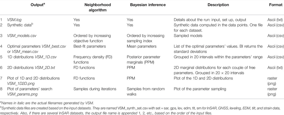
TABLE 3. Output of VSM based on the sampling algorithm selected.

3 Use of VSM

3.1 Modules of VSM

The VSM package is composed of several modules (Figure 3). Necessary files are VSM.py, VSM_search.py, and VSM_forward.py. The core of VSM is VSM.py. It reads the setting of the current run, reads the data, sets up the sampling algorithm, performs the BI, and writes the output listed in Table 3. The NA inversion is performed by the module VSM_search.py. It is not included in the VSM.py main script to keep it as close to the original as possible. The forward models available are collected in VSM_forward.py.

FIGURE 3

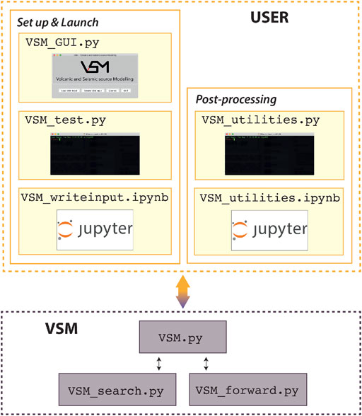
FIGURE 3. Scheme of the VSM modules. VSM.py is the main module for input, computation, and output. It interfaces with VSM_forward.py and VSM_search.py. VSM can be launched by the GUI, by the terminal or any script (e.g., VSM_test.py), and by a Jupyter Notebook script (e.g., VSM_writeinput.ipynb). Post-processing routines are provided in VSM_utilities.py and VSM_utilities.ipynb.

The user can interact with the GUI, VSM_GUI.py. It has been developed based on the Tkinter package (a standard Python interface to the Tk GUI toolkit). Both Tk and Tkinter are available on most Unix platforms and Windows systems. Furthermore, the use of the Tkinter.ttk module provided access to a wider range of Tk-themed widgets, maintaining portability. VSM_writeinput.ipynb is a step-by-step guide to setup the inversion with VSM with explanations and instructions in the Jupyter environment. Finally, an additional file (VSM_utilities.py) is provided to perform post-processing. It contains code to compute the volume variation of a point-source sill-like source (Amoruso and Crescentini, 2013), volume variation of a finite volume sphere and spheroid (Battaglia et al., 2013b), dislocation vertices, and trace coordinates to plot parameter marginals (using a different number of burn-in models or different file formats, e.g., vectorial) and comparisons among observed, calculated, and residual data. Similarly, VSM_utilities.ipynb provides instructions and code to perform such post-processing analysis in the Jupyter environment.

3.2 Detailed Input of VSM

VSM requires a simple text file to run, reporting all the information needed in the correct order. The text is read line-by-line, and Figure 4 reports the screenshot of a typical VSM input file. The first 17 lines are standard, whereas the rest is based on specific choices. The input consists basically of three parts, as shown in the first block of Figure 2: geodetic data input details, forward model setting, and inversion setting.

FIGURE 4

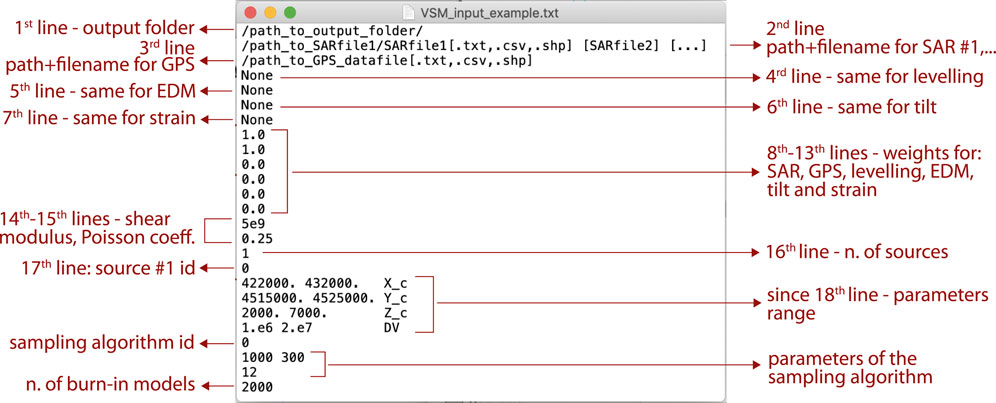
FIGURE 4. Screenshot of a typical VSM text input file with side descriptions. See the list in the main text for detailed explanations.

The structure of the input file for VSM is as follows:

- 1^st line: path to the output folder: the input text file is strongly suggested to be located in the same folder.

- 2^nd–7^th lines: name with a path of each geodetic data file. The order of the six geodetic data types is InSAR, GNSS, leveling, EDM, tilt, and strain data. Lines for lacking data types should report “None.” As VSM supports multiple SAR data files, they should be listed in the same line separated by a space. See Section 2.1 and Table 1 for details on formats and units.

- 8^th–13^th lines: weights assigned to each dataset (the same order as data files).

- 14^th–15^th lines: elastic constants of the medium, shear modulus μ (unit is Pa), and Poisson’s coefficient ν, respectively.

- 16^th line: number of sources composing the forward model.

- 17^th line: source identifier of the (first) chosen analytical source. See details in Section 2.2 and Table 2.

- 18^th line and following: minimum and maximum values of the chosen source’s parameters, in the correct order (see Table 2 and documentation). A third column of text can be added to report the parameters’ name; this is not read by VSM.

- If more than one source is chosen at line 16, additional lines define the source identifier (as in line 17) followed by the related parameters’ ranges (similar to line 18 and following).

- After the forward model setting, a new line defines the choice of the sampling algorithm: 0 for NA or 1 for BI.

- The following two lines define the sampling parameters (Figure 2 and details in Section 2.3). The first line reports the number of samples and the re-sampling for each iteration of NA (p1 and p2), or the number of random walks for BI (p1); the second line identifies the number of iterations for NA (p3), or the number of steps for each random walk for BI (p2).

- The last line defines the number of burn-in samples for the output plots (Table 3 and Section 2.4). This value is arbitrary and aimed at excluding the first part of the search from the plots. Default is 2000; no plots are provided if this value is set to −1. The plot can be re-drawn using the VSM utilities.

This text file can be written by the user in a plain text file or created following the procedure in VSM_writeinput.ipynb (Figure 3) or using the GUI, whose screenshots are shown in Figure 5. After the main window (a), three tabs guide the user to input data (b), forward models (c), and inversion setup (d). Additional pop-ups appear to insert specific information based on the user’s choice.

FIGURE 5

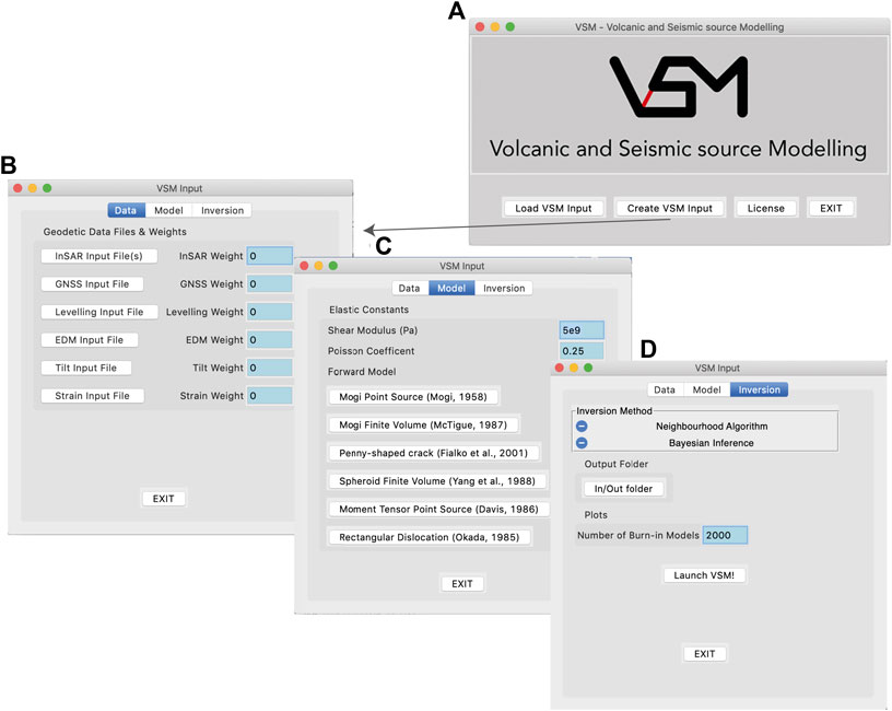
FIGURE 5. (A) Screenshot of the initial window of the GUI and the menu windows for (B) data input, (C) forward models setup, (D) inversion setup.

3.3 How to Launch VSM

There are three ways to launch VSM (Figures 3–5), with or without the input text file described in Section 3.2:

- From a script (e.g., running VSM_test.py) with an input text file.

- By the GUI, launching VSM_GUI.py from a terminal (Figure 5). In this case, VSM can either read an input text file or ingest the setup from the windows.

- By a Jupyter Notebook. There are two notebooks provided. VSM_writeinput.ipynb that writes the VSM input file and launches the VSM. The other, VSM_utilities.ipynb, contains instructions to simply run the code provided that the input file has been already created.

VSM is launched in two steps: the first, using the module VSM.read_VSM_settings(), reads the input text file if this mode is used, and the second launches VSM once the input has been ingested using the module VSM.iVSM(). These instructions are implicit while running the GUI. Regardless of how the input was created and VSM launched, at the end of the run, the log file VSM.log reports in its final lines the VSM-style input text file such as that shown in Figure 4. Furthermore, the VSM setting inserted from the GUI or a Jupyter Notebook is stored in a VSM input text file in the same output folder.

4 Case Study and Comparisons

Extensive testing of VSM is performed on the Campi Flegrei (CF) (Italy) caldera 2011–2013 unrest using all the forward models available. The performance of VSM is tested using a multi-technique dataset consisting of two-orbits InSAR and GPS data, and changing the forward model, the number of unknowns, and the inversion method. All the tests are stored in https://github.com/EliTras/VSM_test and summarized in Table 4. In addition, an application of VSM to the 2011 Van earthquake (Turkey) M7.1 can be found in Trasatti and Tolomei (2022). Further testing on other volcanic areas of the world is collected in Trasatti (2022).

TABLE 4

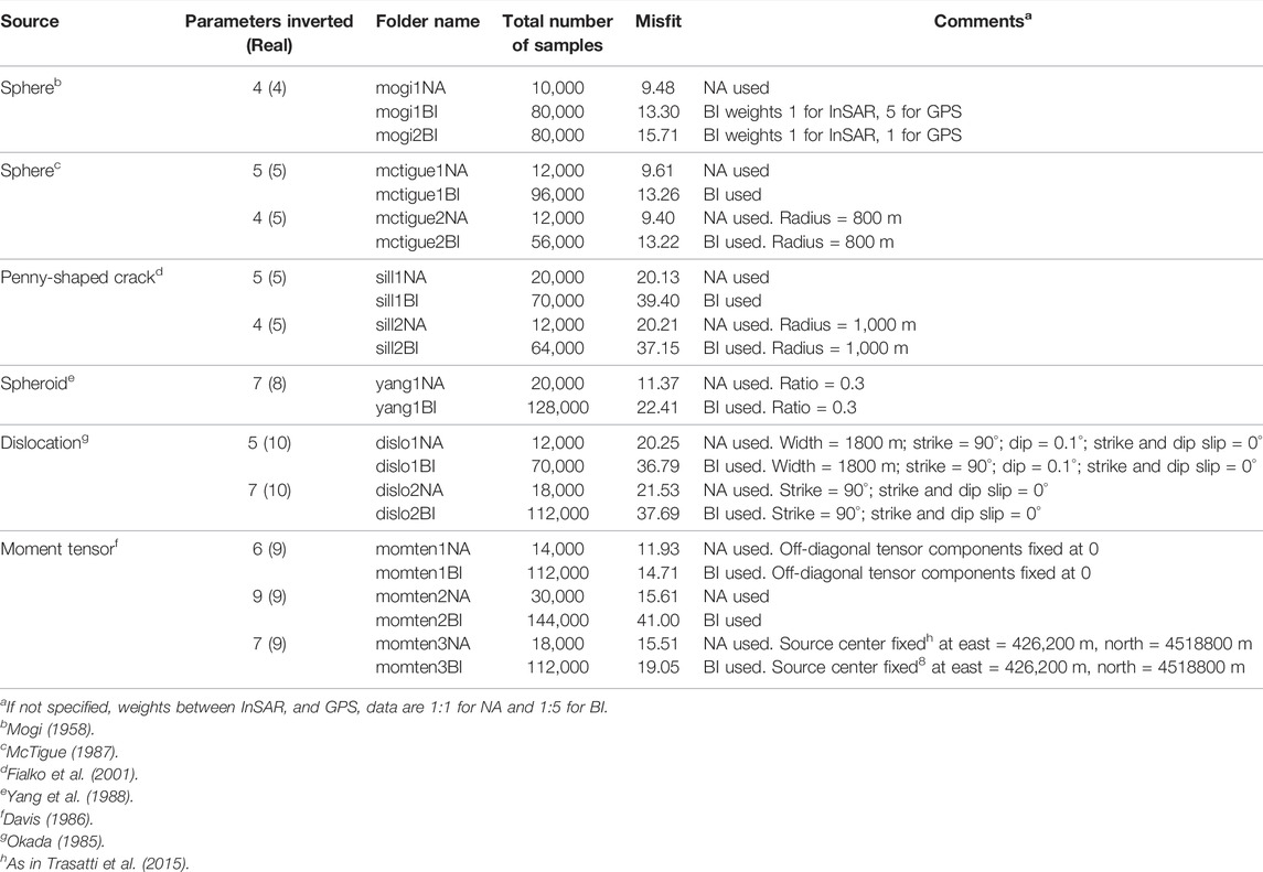
TABLE 4. Details on the tests performed (available at https://github.com/EliTras/VSM_test). The description of the model parameters is reported in Table 2.

Campi Flegrei caldera (Italy) is a volcanic district nearby the city of Naples (Rosi and Sbrana, 1987; Orsi, 2022). Spectacular ground level variations are reported at CF across the centuries, up to tens of meters (Di Vito et al., 2016; Isaia et al., 2019). A large unrest episode occurred during 1982–1984, accompanied by a 1.8 m vertical uplift in Pozzuoli, in the caldera center (Orsi et al., 1996). A slow deflation phase began in 1985, interrupted by minor uplift episodes of a few centimeters, seismic swarms, and degassing episodes. Since 2005, CF has been uplifting again. An increase in the ground velocity occurred during 2011–2013, showing up to 9 cm/yr in 2012 in the caldera center (Amoruso et al., 2014b; D’Auria et al., 2015; Trasatti et al., 2015). We consider the surface deformation obtained by two-orbits datasets of COSMO-SkyMed satellite images (from ASI, the Italian Space Agency) and GPS data from the Neapolitan Volcanoes Continuous GPS (NeVoCGPS) network managed by INGV-Naples related to 2011–2013 (Figure 6). Details about the data analysis are reported in Trasatti et al. (2015). Before using VSM, the InSAR data have been downsampled, consisting of 2,713 and 2,817 data points in the ascending and descending components, respectively. GPS data consist of 3D measurements on 14 benchmarks.

FIGURE 6

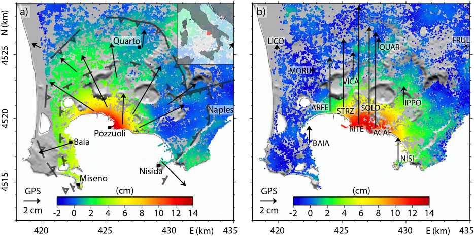
FIGURE 6. LOS cumulative displacements in (A) ascending and (B) descending orbits from the COSMO-SkyMed archive between 31 May 2011 and 5 May 2013 at CF. Horizontal and vertical GPS components are reported in (A) and (B), respectively. In panel a, the outer/inner rims of the CF caldera are shown with open/full triangles. The GPS stations are listed in (B). WGS-84 UTM projection, zone 33.

The data collected are preliminarily inverted by VSM using a Mogi source. The medium is characterized by μ = 5 GPa and ν = 0.25. An issue arising since the first test is the weight to be assigned to the multi-technique datasets, considering that ${\chi }_m^2{}^{null}$ = 30.2 for the InSAR datasets and ${\chi }_m^2{}^{null}=$ 933.8 for GPS data. This 30-fold difference is not surprising because data from GNSS networks have a very low error associated and, therefore, high null chi-square, whereas InSAR data consist of many data points with 1D geometry (LOS) and lower accuracy. The NA inversion, running without a specific weight between InSAR and GPS, provides misfits of 5.1 and 13.7, respectively, with a reduction of misfit of 83.1% for InSAR and 98.6% for GPS (test “mogi1NA”). The likelihood estimation of BI (Eq. 4 and following) differs from the objective function of NA (Eqs 1, 2). This leads to a different misfit computed for the mean set of parameters of BI (test “mogi2BI”), equal to 4.8 for InSAR (84.1% reduction) and 26.6 for GPS (98.5% reduction). In order to obtain a better fit with GPS data, the weights are set to 1 for InSAR and 5 for GPS during the BI (“mogi1BI”), achieving a misfit of 5.0 for InSAR and 15.0 for GPS, similarly to the test with NA. These weights for the BI are kept constant in all the following tests. However, because this choice is arbitrary, other weights among the datasets may be acceptable.

The following data inversions have been performed adopting a sill-like source, according to previous findings at CF (Amoruso et al., 2014a; D’Auria et al., 2015; Trasatti et al., 2015). The tests performed with both NA and BI show similar performance to the samplings (Figure 7). The BI parameter marginal distributions are less scattered with respect to NA. Both samplings reveal a hyperbolic trade-off between the radius and ΔP/μ. The corresponding tests are “sill1NA” and “sill1BI.” Data cannot constrain these parameters univocally because the marginal distributions evidence their nearly hyperbolic relationship. Values within the 2D high-density area provide a statistically equivalent data fit. Consequently, because this area is in the range of 600–1,400 m for the radius, the radius is fixed at 1 km. The tests running with the remaining four free parameters of the sill are set with 12 iterations and 1,000 samplings (and 300 re-samplings) for NA, and 8 random walks and 8,000 steps for BI. Therefore, a total of 12,000 and 64,000 models are generated by NA and BI, respectively. These tests (“sill2NA” and “sill2BI”) are also accompanied by Jupyter Notebooks (available at https://github.com/EliTras/VSM_test/tree/main/USECASE/sill2NA and https://github.com/EliTras/VSM_test/tree/main/USECASE/sill2BI). The resulting reduced chi-square misfits amount to 5.8 for InSAR and 34.7 for GPS (20.2 in total) for NA, and 4.5 for InSAR and 43.7 for GPS (37.1 in total) for BI. The BI provides a higher misfit, but the reduced chi-square is computed a posteriori as an indicator of goodness of fit, and it is not actually ruling the sampling. The results are reported in Figure 8 and Table 5. The uncertainty associated with each best-fit parameter for the NA inversion has been computed from the half-width of the frequency density (e.g., Sambridge, 1999b; Trasatti et al., 2015), whereas mean values and standard deviations are a result supplied by the BI.

FIGURE 7

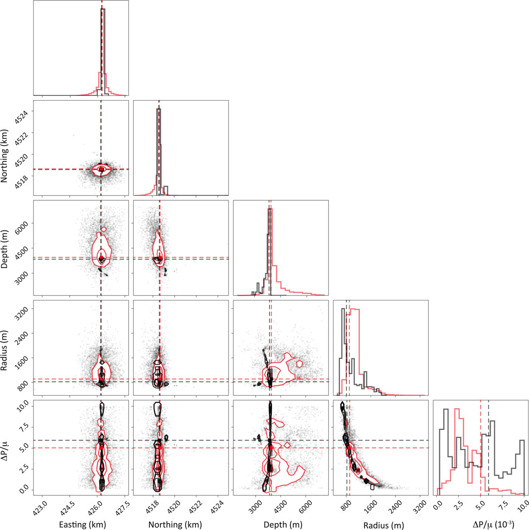
FIGURE 7. Summary of the 1D and 2D parameter marginal distributions for NA (red lines, best-fit dashed lines) and BI (black lines, mean parameters dashed lines) for the sill-like source (Fialko et al., 2001) with all the five parameters estimated. Corresponding tests are “sill1NA” and “sill1BI.”

FIGURE 8

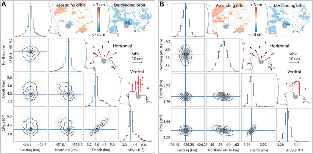
FIGURE 8. Summary of the VSM results for NA [group (A)] and BI [group (B)]. 1D and 2D parameter marginal distributions and comparisons with data. The maps show the residuals (data minus optimal model) with the InSAR data, whereas GPS data and model are reported with black and red arrows, respectively. The sill-like source is reported with an in-scale grey circle on the maps.

TABLE 5

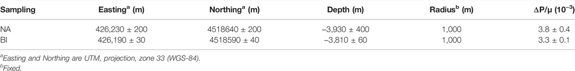
TABLE 5. Results of the VSM inversions of the sill-like source at CF using NA and BI.

Both inversions retrieve a sill located beneath Pozzuoli, at slightly less than 4 km depth. The inverted parameters are compatible with their uncertainty. In particular, sill centers are almost coincident, whereas a larger relative uncertainty affects the ΔP/μ estimate. Similarly, the volume variation amounts to ΔV = 7.6 ± 0.8 10⁶ m³ for NA and 6.6 ± 0.2 10⁶ m³ for BI. These results are compatible with previous findings for the same period (Amoruso et al., 2014a; D’Auria et al., 2015; Trasatti et al., 2015). Figure 8 shows the 1D and 2D parameter marginals obtained by NA and BI. The 1D parameter distributions are characterized by single-density maximum and the presence of a limited trade-off with positive trending between depth and ΔP/μ. The BI inversion retrieves distributions much more concentrated on the global minimum than the NA, as reported in Figure 7. Therefore, the BI inversion is very focused, and the associated standard deviation is lower than the uncertainty retrieved by NA. As a result, the parameters retrieved by the two inversions show uncertainties scaling by even one order of magnitude (Table 5). The standard deviations are actually very small, amounting to a few tens of meters for the source center position. From one side, it means that the MCMC sampling method converges faster to the global minimum zone than the direct search of the Voronoi cells. On the contrary, in the case of a higher number of parameters, a lack of exploration of BI cannot be excluded, with potential trapping in local minima of the parameter space.

Figure 8 shows comparisons between observed and synthetic data. NA and BI similarly fit the data. The ascending dataset shows a better fit in average than the descending one because positive and negative residuals are present. However, the descending orbit data are mainly overestimated, with a predominance of blue in the residuals. The GPS measurements are reproduced with similar performances.

4.1 Performance of VSM

The performance of VSM is tested with a total of 22 runs implementing the six forward models available and different settings, using both NA and BI (Table 4). All the runs are performed using an Apple iMac (processor 4 GHz Intel core i7, memory 16 GB DDR3 1,600 MHz). Inversions are set up to avoid as much as possible to trap into one of the potentially multiple local minima. The tests are performed considering a conservative number of total samples generated to evidence the similarities and differences between the NA and BI. To perform a fruitful search of the parameter space, in some inversions, the number of free parameters has been lowered or their range narrowed.

Figure 9 reports the results of the inversion in terms of performance, considering the number of parameters, the type of the forward model, and the misfit for each type of data for NA and BI. The execution time (Figure 9A) is very low for simplified analytical formulations such as the point-source sphere, the finite volume sphere, and the moment tensor. However, it increases for forward models with more complex analytical formulations such as dislocation and spheroid, with the largest computational time required by the penny-shaped crack involving numerical integration. In general, for the same forward model, if one or more parameters are fixed, the execution time reduces. Furthermore, the NA inversion systematically requires a longer execution than the BI; even if to obtain acceptable parameter marginals, the NA needs fewer samplings. In the tests discussed, the ratio between the total samples for similar tests generated by BI versus NA is between 3.5 and 8. Figure 9B shows that the misfit of GPS data (open squares and diamonds) is systematically worse than with InSAR (full squares and diamonds), not surprising due to the null test discussed above, evidencing the higher signal-to-noise ratio of the GPS dataset. BI inversions also provide misfits with GPS systematically worse than NA (open diamonds and open squares, respectively), evidencing the need for weight among GPS and InSAR and suggesting that weights even higher than five may have been associated with GPS. This feature is not so evident for InSAR data because the misfits are quite low and range between 3.8 and 6.0.

FIGURE 9

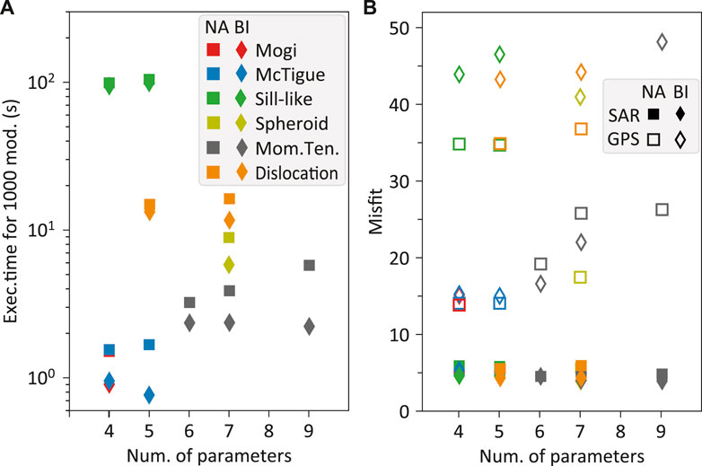
FIGURE 9. Comparisons among different forward models using the NA and BI. (A) Execution time for 1,000 samples versus the number of parameters. The same forward model is used with some parameters fixed. (B) Comparisons among misfits from NA and BI considering InSAR and GPS data. Colors for the sources are as in (A).

Figure 10 gathers the optimal parameters from most of the inversions. The volume variation is derived using the VSM utilities for all the sources except for Mogi because it is one of the inverted parameters. The uncertainty is computed from those associated with the parameters involved by error propagation. For the dislocation model, the center and its uncertainty are derived from its top-left corner and dimensions. The results from the moment tensor source require further analysis to retrieve the principal moment values and obtain the volume variation of the equivalent ellipsoid (Amoruso and Crescentini, 2013). The parameters and the volume variation are affected by large uncertainties. Therefore, only the tests with Easting and Northing fixed are shown. In Figure 10, the retrieved geographical locations of all the sources are compatible within the confidence interval included in a range of variability of 160 and 360 m, respectively. For all the models presented, depth and volume variation show larger fluctuations. The depth ranges from 2,600 to 2,700 m (spherical sources), 2,900 m of the spheroidal source, and 3,000–3,500 m for the moment tensor (the latter with large uncertainty) to about 3,900 m for sill and dislocation based on the different settings. The shallower depths retrieved by the isotropic finite volume or point sources with respect to other model geometries are already known (Trasatti et al., 2011). Accordingly, a similar variability can be observed for the volume variation. Sources such as sill and dislocation, being deeper, have larger volume variation associated with respect to the spherical and spheroidal sources. The difference in the retrieved volume variations is outside the parameter uncertainty associated and amounts to 30%–40%. The derived volume variations for the equivalent ellipsoid are within the values retrieved by the other sources, although affected by large uncertainties. As a last comment, the different sampling methods do not show biases in the retrieved optimal parameters. Results obtained with the same forward model and parameters setting performed by NA or BI are compatible. It is confirmed that BI retrieves much smaller confidence ranges with respect to NA, as already pointed out in Figures 7, 8.

FIGURE 10

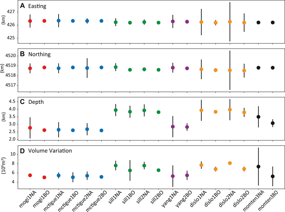
FIGURE 10. Retrieval of the (A) east and (B) north coordinates of the source center, (C) depth, and (D) volume variation by NA and BI, based on different forward models and setting (the labels in the abscissa refer to the test names). Details in Table 4.

4.2 Choice of the Inversion Method

The choice of using NA or BI and its specific setting is made by the user. Nevertheless, the suggested best practice is to perform several runs with both, comparing and cross-checking the results. For approximately the same number of models generated, NA offers a wider search of the parameter space and a shorter execution time. On the other side, it may reach the global minimum more slowly. Generally, the BI should be set up with a number of walks greater than twice the number of free parameters. Nevertheless, the execution time of BI is usually longer than NA because the sampling requires many walks and many steps, amounting to several times the samples generated by a reasonably good NA inversion, considering the same data and forward model settings. These comments are very general because each dataset, number of data points, and signal-to-noise ratio rule the inversion process in a different and nearly unpredictable way. Furthermore, the global minimum may be very or poorly attractive, or there may be several minima equally fitting the data, or there may be a wide range of models with similar significance in terms of data fitting. Akaike’s information criterion (AIC) can compare the quality of a set of statistical models to each other (Akaike, 1974). It may address the significance of improvement/worsening of data fit using a different number of parameters or different forward sources among those available in VSM.

The combination of multiple datasets and arbitrary weights has different impacts on the NA and BI due to the intrinsic difference in the approach and sampling algorithm. The case study has shown that different weights between InSAR and GPS in NA and BI were required to achieve a similar level of data fitting. In general, after enough attempts, the results of both methods should converge to compatible global minima, as shown in Figure 10, if the runs are adequately set up. The comparison among chi-squares obtained with different setups and with the null chi-square (see Section 2.3.1 and Table 4) is another indicator of the suitability of the chosen setting for the inversions. Because the null chi-square is a measure of the signal-to-noise ratio of each given dataset, it may help select the relative weights in the case of multiple datasets, as discussed in the application at CF for InSAR and GPS data. Leveling data are often characterized by low uncertainty associated and, therefore, a high ${\chi }_m^2{}^{null}$, requiring a careful choice of the weight if adopted in combination with other datasets. First-derivative data such as borehole tilt and strain are very sensitive to source migration. Usually, they are treated with particular care and not in conjunction with other geodetic data or with continuous GPS data at the most (Aloisi et al., 2020).

5 Discussion and Conclusion

VSM is an open-source Python tool to model ground deformations detected by many satellites and ground geodetic techniques, implementing the most common analytical source models used for this purpose. VSM provides geophysical scientists a user-friendly and practical toolkit to perform geophysical inversion modeling using Python scripts, the Jupyter Notebooks environment, or its GUI. VSM is available on GitHub (https://github.com/EliTras/VSM).

Recently, data assimilation techniques have been applied to InSAR data of volcanic and seismic areas (Bato et al., 2017; Rouet-Leduc et al., 2021). The huge amount of information from InSAR data is suitable for sequential data assimilation to disclose the temporal evolution of the deformation signal in areas characterized by natural hazards. The VSM tool is ready for data-driven applications, and its routines can be implemented in machine learning algorithms. Other planned future developments of the VSM code include the implementation of pre-processing routines for semi-automatic InSAR data downsampling, incorporation of Digital Elevation Models to account for topography, improvement of the GUI, and setup for near real-time applications. A possible further development may include linear inversions of slip distributions on faults and other deformation source models, such as the Compound Dislocation Model, composed of three mutually orthogonal rectangular dislocations with full rotational degrees of freedom (Nikkhoo et al., 2017). Finally, deformation and gravity changes are expected to correlate (e.g., magma/fluid intrusion or deployment causes surface gravity changes). VSM may be extended to account for additional forward analytical deformation models and gravity data by adding the related few analytical sources available (Trasatti and Bonafede, 2008; Nikkhoo and Rivalta, 2022).

The data covariance matrix is assumed as diagonal in VSM. This assumption may be an over-simplification for InSAR deformation data, which are typically affected by correlated errors. Neglecting these can impact the source parameter estimates (Sudhaus and Jónsson, 2009) because they affect the normalization of the likelihoods. In VSM, the weights among datasets and, therefore, the likelihood normalization are defined by the user. A planned development of VSM includes the implementation of hierarchical Bayesian inference to assess formal dataset weight determination (Bodin et al., 2012). This would avoid the definition of weights among datasets by the user. Moreover, the treatment of data covariance is one of the planned developments.

Surface deformations may originate from several phenomena occurring in the same area or region (e.g., volcanic and tectonic activity). Therefore, data inversion should consider any potential sources of deformation and model them accordingly, or, conversely, other signals not reproducible by the available forward models (e.g., a tectonic trend known by other studies) may be removed from the input data before the inversions (Silverii et al., 2021). Furthermore, local effects such as lava flow cooling (usually giving coherent patterns with InSAR) should be masked out. Geophysical prospecting and seismic tomography disclose structural heterogeneities of the crust that are not accounted for in the analytical models implemented in tools such as VSM. Nevertheless, this information can be considered in the model setup to fix the position and/or depth of the deformation source or shrink the parameter range. Indications from geophysical, volcanological, and geochemical studies may help define the position and/or shape of the source. Consequently, the inversions based on geodetic data may not retrieve the absolute minimum misfit because some parameters are constrained by independent data, but the results will be compatible with a priori knowledge of the area. In this way, analytical models are still largely used because they are easy to run and provide fast results that may be used in operative frameworks. Indeed, in the case of an earthquake, forward models may be generated from the first information available, for example, from the focal mechanism and using standard relationships (Wells and Coppersmith, 1994) to define the fault parameters. As soon as geodetic data are available, fast or preliminary data inversion may help localize the trace of the fault. The same applies to volcanic areas using continuous GNSS or borehole monitoring data to track magma intrusion (Cannavò et al., 2015; Beauducel et al., 2020).

To conclude, any emergency, being related to geohazards such as volcanic eruptions and earthquakes, or the global sanitary emergency started in 2020, prove that the need for open science is a matter of fact. Similarly, more transparency on how scientific knowledge is created, especially when science should guide crucial decisions affecting thousands to millions of people should be common practice. The FAIR (Findable, Accessible, Interoperable, Reusable, Wilkinson et al., 2016) principles have become reference criteria for scientific data management, also in the field of Earth Science. These criteria apply to a certain extent to any aspect of the scientific research cycle (Garcia-Silva et al., 2019; Bailo et al., 2020). Service resources such as open tools for scientific purposes and for operative frameworks with near real-time implementation are part of this ecosystem. VSM is inspired and compliant to these principles. The massive availability of remote sensing data, especially those open access (e.g., ESA’s Sentinel missions) or provided in the framework of global initiatives such as GEO-GSNL (Geohazard Supersites and National Laboratories https://geo-gsnl.org/), gave rise to a growing number of services for data analysis (e.g., the Alaskan Facility Service, the Geohazard Exploitation Platform or the LiCSBAS, Morishita et al., 2020). The future must embrace routine data exploitation, developing analysis capabilities of larger communities and sustaining the flow with international cooperation (Fernández et al., 2017). Modelling tools such as VSM are services to fully exploit these scientific products in many domains of Earth Science, from advanced scientific research to outreach, from implementation of near real-time monitoring data to under-monitored high-risk volcanic and seismic areas of the world.

Data Availability Statement

The original contributions presented in the study are included in the article/Supplementary Material. Further inquiries can be directed to the corresponding author.

Author Contributions

The author confirms being the sole contributor to this work and has approved it for publication.

Funding

This work was jointly supported by the “Research Lifecycle Management technologies for Earth Science Communities and Copernicus users in EOSC” Reliance project funded by the European Commission’s H2020 2021-2022 (Grant Agreement no. 101017501); Pianeta Dinamico—Working Earth project (2020-2030) funded by the Italian Ministry of University and Research (Decree no. 1118 04/12/2019); and “Linking Surface Observables to sub-Volcanic Plumbing-System: A Multidisciplinary Approach for Eruption Forecasting at Campi Flegrei Caldera (Italy)” LOVE-CF (2020-2023) project funded by INGV (Internal Register no. 1865 17/07/2020).

Conflict of Interest

The authors declare that the research was conducted in the absence of any commercial or financial relationships that could be construed as a potential conflict of interest.

Publisher’s Note

All claims expressed in this article are solely those of the authors and do not necessarily represent those of their affiliated organizations or those of the publisher, the editors, and the reviewers. Any product that may be evaluated in this article, or claim that may be made by its manufacturer, is not guaranteed or endorsed by the publisher.

Acknowledgments

The author acknowledges N. Piana Agostinetti for the first version of the Fortran code for the useful discussions on data inversion and this manuscript. Thanks to M. Sambridge for providing the NA Fortran code. In the last 15 years, the development of the code has been encouraged at different times by S. Salvi, M. Battaglia, M. Bonafede, and C. Giunchi. The Python version of VSM benefited from suggestions by D. Stelitano, F. Zanolin, N. Svigkas, and E. Casarotti. COSMO-SkyMed raw data processed by M. Polcari.

References

Agnew, D. C. (1986). Strainmeters and Tiltmeters. Rev. Geophys. 24, 579–624. doi:10.1029/RG024i003p00579

CrossRef Full Text | Google Scholar

Akaike, H. (1974). A New Look at the Statistical Model Identification. IEEE Trans. Autom. Contr. 19, 716–723. doi:10.1109/TAC.1974.1100705

CrossRef Full Text | Google Scholar

Aloisi, M., Bonaccorso, A., Cannavò, F., Currenti, G., and Gambino, S. (2020). The 24 December 2018 Eruptive Intrusion at Etna Volcano as Revealed by Multidisciplinary Continuous Deformation Networks (CGPS, Borehole Strainmeters and Tiltmeters). JGR Solid Earth 125 (8), e2019JB019117. doi:10.1029/2019JB019117

CrossRef Full Text | Google Scholar

Amoruso, A., Crescentini, L., Sabbetta, I., De Martino, P., Obrizzo, F., and Tammaro, U. (2014b). Clues to the Cause of the 2011-2013 Campi Flegrei Caldera Unrest, Italy, from Continuous GPS Data. Geophys. Res. Lett. 41, 3081–3088. doi:10.1002/2014GL059539

CrossRef Full Text | Google Scholar

Amoruso, A., Crescentini, L., and Sabbetta, I. (2014a). Paired Deformation Sources of the Campi Flegrei Caldera (Italy) Required by Recent (1980-2010) Deformation History. J. Geophys. Res. Solid Earth 119, 858–879. doi:10.1002/2013JB010392

CrossRef Full Text | Google Scholar

Antonella Amoruso, A., and Luca Crescentini, L. (2013). Analytical Models of Volcanic Ellipsoidal Expansion Sources. Ann. Geophys 56. doi:10.4401/ag-6441

CrossRef Full Text | Google Scholar

Bagnardi, M., and Hooper, A. (2018). Inversion of Surface Deformation Data for Rapid Estimates of Source Parameters and Uncertainties: A Bayesian Approach. Geochem. Geophys. Geosyst. 19, 2194–2211. doi:10.1029/2018GC007585

CrossRef Full Text | Google Scholar

Bailo, D., Paciello, R., Sbarra, M., Rabissoni, R., Vinciarelli, V., and Cocco, M. (2020). Perspectives on the Implementation of FAIR Principles in Solid Earth Research Infrastructures. Front. Earth Sci. 8, 3. doi:10.3389/feart.2020.00003

CrossRef Full Text | Google Scholar

Bato, M. G., Pinel, V., and Yan, Y. (2017). Assimilation of Deformation Data for Eruption Forecasting: Potentiality Assessment Based on Synthetic Cases. Front. Earth Sci. 5, 48. doi:10.3389/feart.2017.00048

CrossRef Full Text | Google Scholar

Battaglia, M., Cervelli, P. F., and Murray, J. R. (2013a). DMODELS: A MATLAB Software Package for Modeling Crustal Deformation Near Active Faults and Volcanic Centers. J. Volcanol. Geotherm. Res. 254, 1–4. doi:10.1016/j.jvolgeores.2012.12.018

CrossRef Full Text | Google Scholar

Battaglia, M., Cervelli, P. F., and Murray, J. R. (2013b). Modeling Crustal Deformation Near Active Faults and Volcanic Centers—A Catalog of Deformation Models. Available at: http://pubs.er.usgs.gov/publication/tm13B1.

Google Scholar

Beauducel, F., Peltier, A., Villié, A., and Suryanto, W. (2020). Mechanical Imaging of a Volcano Plumbing System from GNSS Unsupervised Modeling. Geophys. Res. Lett. 47 (17), e2020GL089419. doi:10.1029/2020GL089419

CrossRef Full Text | Google Scholar

Bianchi, I., Piana Agostinetti, N., De Gori, P., and Chiarabba, C. (2008). Deep Structure of the Colli Albani Volcanic District (Central Italy) from Receiver Functions Analysis. J. Geophys. Res. 113. doi:10.1029/2007JB005548

CrossRef Full Text | Google Scholar

Biggs, J., Ebmeier, S. K., Aspinall, W. P., Lu, Z., Pritchard, M. E., Sparks, R. S. J., et al. (2014). Global Link between Deformation and Volcanic Eruption Quantified by Satellite Imagery. Nat. Commun. 5, 3471. doi:10.1038/ncomms4471

PubMed Abstract | CrossRef Full Text | Google Scholar

Biggs, J., and Wright, T. J. (2020). How Satellite InSAR Has Grown from Opportunistic Science to Routine Monitoring over the Last Decade. Nat. Commun. 11, 3863. doi:10.1038/s41467-020-17587-6

PubMed Abstract | CrossRef Full Text | Google Scholar

Bodin, T., Sambridge, M., Rawlinson, N., and Arroucau, P. (2012). Transdimensional Tomography with Unknown Data Noise. Geophys. J. Int. 189, 1536–1556. doi:10.1111/j.1365-246X.2012.05414.x

CrossRef Full Text | Google Scholar

Cannavò, F. (2019). A New User-Friendly Tool for Rapid Modelling of Ground Deformation. Comput. Geosciences 128, 60–69. doi:10.1016/j.cageo.2019.04.002

CrossRef Full Text | Google Scholar

Cannavò, F., Camacho, A. G., González, P. J., Mattia, M., Puglisi, G., and Fernández, J. (2015). Real Time Tracking of Magmatic Intrusions by Means of Ground Deformation Modeling during Volcanic Crises. Sci. Rep. 5, 10970. doi:10.1038/srep10970

PubMed Abstract | CrossRef Full Text | Google Scholar

Chen, B., Li, Z., Yu, C., Fairbairn, D., Kang, J., Hu, J., et al. (2020). Three-dimensional Time-Varying Large Surface Displacements in Coal Exploiting Areas Revealed through Integration of SAR Pixel Offset Measurements and Mining Subsidence Model. Remote Sens. Environ. 240, 111663. doi:10.1016/j.rse.2020.111663

CrossRef Full Text | Google Scholar

Colesanti, C., and Wasowski, J. (2006). Investigating Landslides with Space-Borne Synthetic Aperture Radar (SAR) Interferometry. Eng. Geol. 88, 173–199. doi:10.1016/j.enggeo.2006.09.013

CrossRef Full Text | Google Scholar

D’Auria, L., Pepe, S., Castaldo, R., Giudicepietro, F., Macedonio, G., Ricciolino, P., et al. (2015). Magma Injection beneath the Urban Area of Naples: A New Mechanism for the 2012-2013 Volcanic Unrest at Campi Flegrei Caldera. Sci. Rep. 5, 1–11. doi:10.1038/srep13100

CrossRef Full Text | Google Scholar

Davis, P. M. (1986). Surface Deformation Due to Inflation of an Arbitrarily Oriented Triaxial Ellipsoidal Cavity in an Elastic Half-Space, with Reference to Kilauea Volcano, Hawaii. J. Geophys. Res. 91, 7429–7438. doi:10.1029/jb091ib07p07429

CrossRef Full Text | Google Scholar

DeMets, C., Gordon, R. G., Argus, D. F., and Stein, S. (1990). Current Plate Motions. Geophys. J. Int. 101, 425–478. doi:10.1111/j.1365-246X.1990.tb06579.x

CrossRef Full Text | Google Scholar

Di Vito, M. A., Acocella, V., Aiello, G., Barra, D., Battaglia, M., Carandente, A., et al. (2016). Magma Transfer at Campi Flegrei Caldera (Italy) before the 1538 AD Eruption. Sci. Rep. 6, 32245. doi:10.1038/srep32245

PubMed Abstract | CrossRef Full Text | Google Scholar

Eshelby, J. D. (1957). The Determination of the Elastic Field of an Ellipsoidal Inclusion, and Related Problems. Proc. R. Soc. Lond. A 241, 376–396. doi:10.1098/rspa.1957.0133

CrossRef Full Text | Google Scholar

Fernández, J., Pepe, A., Poland, M. P., and Sigmundsson, F. (2017). Volcano Geodesy: Recent Developments and Future Challenges. J. Volcanol. Geotherm. Res. 344, 1–12. doi:10.1016/j.jvolgeores.2017.08.006

CrossRef Full Text | Google Scholar

Fialko, Y., Khazan, Y., and Simons, M. (2001). Deformation Due to a Pressurized Horizontal Circular Crack in an Elastic Half-Space, with Applications to Volcano Geodesy. Geophys. J. Int. 146, 181–190. doi:10.1046/j.1365-246X.2001.00452.x

CrossRef Full Text | Google Scholar

Foreman-Mackey, D., Hogg, D. W., Lang, D., and Goodman, J. (2013). Emcee: The MCMC Hammer. Publ. Astronomical Soc. Pac. 125, 306–312. doi:10.1086/670067

CrossRef Full Text | Google Scholar

Galloway, D. L., and Hoffmann, J. (2007). The Application of Satellite Differential SAR Interferometry-Derived Ground Displacements in Hydrogeology. Hydrogeol. J. 15, 133–154. doi:10.1007/s10040-006-0121-5

CrossRef Full Text | Google Scholar

Garcia-Silva, A., Gomez-Perez, J. M., Palma, R., Krystek, M., Mantovani, S., Foglini, F., et al. (2019). Enabling FAIR Research in Earth Science through Research Objects. Future Gener. Comput. Syst. 98, 550–564. doi:10.1016/j.future.2019.03.046

CrossRef Full Text | Google Scholar

Geman, S., and Geman, D. (1984). Stochastic Relaxation, Gibbs Distributions, and the Bayesian Restoration of Images. IEEE Trans. Pattern Anal. Mach. Intell. PAMI-6, 721–741. doi:10.1109/TPAMI.1984.4767596

PubMed Abstract | CrossRef Full Text | Google Scholar

Goodman, J., and Weare, J. (2010). Commun. Appl. Math. Comput. Sci. Available at: https://msp.org/camcos/2010/5-1/camcos-v5-n1-p04-p.pdf.

Google Scholar

Hashimoto, C., Noda, A., Sagiya, T., and Matsu’ura, M. (2009). Interplate Seismogenic Zones along the Kuril-Japan Trench Inferred from GPS Data Inversion. Nat. Geosci. 2, 141–144. doi:10.1038/ngeo421

CrossRef Full Text | Google Scholar

Heimann, S., Vasyura-Bathke, H., Sudhaus, H., Isken, M. P., Kriegerowski, M., Steinberg, A., et al. (2019). A Python Framework for Efficient Use of Pre-computed Green's Functions in Seismological and Other Physical Forward and Inverse Source Problems. Solid earth. 10, 1921–1935. doi:10.5194/se-10-1921-2019

CrossRef Full Text | Google Scholar

Isaia, R., Vitale, S., Marturano, A., Aiello, G., Barra, D., Ciarcia, S., et al. (2019). High-resolution Geological Investigations to Reconstruct the Long-Term Ground Movements in the Last 15 Kyr at Campi Flegrei Caldera (Southern Italy). J. Volcanol. Geotherm. Res. 385, 143–158. doi:10.1016/j.jvolgeores.2019.07.012

CrossRef Full Text | Google Scholar

Kennett, B. L. N., Marson-Pidgeon, K., and Sambridge, M. S. (2000). Seismic Source Characterization Using a Neighbourhood Algorithm. Geophys. Res. Lett. 27, 3401–3404. doi:10.1029/2000GL011559

CrossRef Full Text | Google Scholar

Lisowski, M. (2007). “Analytical Volcano Deformation Source Models,” in Volcano Deformation (Berlin, Heidelberg: Springer), 279–304. doi:10.1007/978-3-540-49302-0_8

CrossRef Full Text | Google Scholar

Lohman, R. B., and Simons, M. (2005). Some Thoughts on the Use of InSAR Data to Constrain Models of Surface Deformation: Noise Structure and Data Downsampling. Geochem. Geophys. Geosyst. 6, a–n. doi:10.1029/2004GC000841

CrossRef Full Text | Google Scholar

Masterlark, T. (2007). Magma Intrusion and Deformation Predictions: Sensitivities to the Mogi Assumptions. J. Geophys. Res. 112. doi:10.1029/2006JB004860

CrossRef Full Text | Google Scholar

McTigue, D. F. (1987). Elastic Stress and Deformation Near a Finite Spherical Magma Body: Resolution of the Point Source Paradox. J. Geophys. Res. 92, 12931. doi:10.1029/jb092ib12p12931

CrossRef Full Text | Google Scholar

Mindlin, R. D. (1936). Force at a Point in the Interior of a Semi‐Infinite Solid. Physics 7, 195–202. doi:10.1063/1.1745385

CrossRef Full Text | Google Scholar

Mogi, K. (1958). Relations between the Eruptions of Various Volcanoes and the Deformations of the Ground Surfaces Around Them. Bull. Earthq. Res. Inst. 36, 99–134.

Google Scholar

Morishita, Y., Lazecky, M., Wright, T., Weiss, J., Elliott, J., and Hooper, A. (2020). LiCSBAS: An Open-Source Insar Time Series Analysis Package Integrated with the LiCSAR Automated Sentinel-1 InSAR Processor. Remote Sens. 12, 424. doi:10.3390/rs12030424

CrossRef Full Text | Google Scholar

Mosegaard, K., and Tarantola, A. (1995). Monte Carlo Sampling of Solutions to Inverse Problems. J. Geophys. Res. 100, 12431–12447. doi:10.1029/94jb03097

CrossRef Full Text | Google Scholar

Nikkhoo, M., and Rivalta, E. (2022). Analytical Solutions for Gravity Changes Caused by Triaxial Volumetric Sources. Geophys. Res. Lett. 49, 1–17. doi:10.1029/2021gl095442

CrossRef Full Text | Google Scholar

Nikkhoo, M., Walter, T. R., Lundgren, P. R., and Prats-Iraola, P. (2017). Compound Dislocation Models (CDMs) for Volcano Deformation Analyses. Geophys. J. Int. 208, 877–894. doi:10.1093/gji/ggw427

CrossRef Full Text | Google Scholar

Okada, Y. (1985). Surface Deformation Due to Shear and Tensile Faults in a Half-Space. Int. J. Rock Mech. Min. Sci. Geomech. Abstr. 75, 1135–1154. doi:10.1785/bssa0750041135

CrossRef Full Text | Google Scholar

Orsi, G., De Vita, S., and Di Vito, M. (1996). The Restless, Resurgent Campi Flegrei Nested Caldera (Italy): Constraints on its Evolution and Configuration. J. Volcanol. Geotherm. Res. 74, 179–214. doi:10.1016/S0377-0273(96)00063-7

CrossRef Full Text | Google Scholar

Orsi, G. (2022). “Volcanic and Deformation History of the Campi Flegrei Volcanic Field, Italy,” in Active Volcanoes of the World, 1–53. doi:10.1007/978-3-642-37060-1_1

CrossRef Full Text | Google Scholar

Poland, M. P., and de Zeeuw-van Dalfsen, E. (2021). “Volcano Geodesy: A Critical Tool for Assessing the State of Volcanoes and Their Potential for Hazardous Eruptive Activity,” in Forecasting and Planning for Volcanic Hazards, Risks, and Disasters (Amsterdam, Netherlands: Elsevier), 75–115. doi:10.1016/b978-0-12-818082-2.00003-2

CrossRef Full Text | Google Scholar

Reading, A., Kennett, B., and Sambridge, M. (2003). Improved Inversion for Seismic Structure Using transformed,S-Wavevector Receiver Functions: Removing the Effect of the Free Surface. Geophys. Res. Lett. 30 (19). doi:10.1029/2003GL018090

CrossRef Full Text | Google Scholar

Rosi, M., and Sbrana, A. (1987). The Phlegrean Fields. Rome: Quaderni “La Ricerca Scientifica”CNR.

Google Scholar

Rouet-Leduc, B., Jolivet, R., Dalaison, M., Johnson, P. A., and Hulbert, C. (2021). Autonomous Extraction of Millimeter-Scale Deformation in InSAR Time Series Using Deep Learning. Nat. Commun. 12, 6480. doi:10.1038/s41467-021-26254-3

PubMed Abstract | CrossRef Full Text | Google Scholar

Sambridge, M. (1999b). Geophysical Inversion with a Neighbourhood Algorithm-II. Appraising the Ensemble. Geophys. J. Int. 138, 727–746. doi:10.1046/j.1365-246x.1999.00900.x

CrossRef Full Text | Google Scholar

Sambridge, M. (1999a). Geophysical Inversion with a Neighbourhood Algorithm-I. Searching a Parameter Space. Geophys. J. Int. 138, 479–494. doi:10.1046/j.1365-246X.1999.00876.x

CrossRef Full Text | Google Scholar

Saroli, M., Albano, M., Atzori, S., Moro, M., Tolomei, C., Bignami, C., et al. (2021). Analysis of a Large Seismically Induced Mass Movement after the December 2018 Etna Volcano (Southern Italy) Seismic Swarm. Remote Sens. Environ. 263, 112524. doi:10.1016/j.rse.2021.112524

CrossRef Full Text | Google Scholar

Segall, P. (2010). Earthquake and Volcano Deformation. New Jersey, United States: Princeton Univeristy Press. doi:10.1515/9781400833856

CrossRef Full Text | Google Scholar

Shirzaei, M., and Bürgmann, R. (2018). Global Climate Change and Local Land Subsidence Exacerbate Inundation Risk to the San Francisco Bay Area. Sci. Adv. 4, eaap9234. doi:10.1126/sciadv.aap9234

PubMed Abstract | CrossRef Full Text | Google Scholar

Silverii, F., Pulvirenti, F., Montgomery-Brown, E. K., Borsa, A. A., and Neely, W. R. (2021). The 2011-2019 Long Valley Caldera Inflation: New Insights from Separation of Superimposed Geodetic Signals and 3D Modeling. Earth Planet. Sci. Lett. 569, 117055. doi:10.1016/j.epsl.2021.117055

CrossRef Full Text | Google Scholar

Snoke, J. A. (2002). Constraints on theSwave Velocity Structure in a Continental Shield from Surface Wave Data: Comparing Linearized Least Squares Inversion and the Direct Search Neighbourhood Algorithm. J. Geophys. Res. 107 (B5), ESE 4-1–ESE 4-8. doi:10.1029/2001jb000498

CrossRef Full Text | Google Scholar

Sparks, R. S., Biggs, J., and Neuberg, J. W. (2012). Geophysics. Monitoring Volcanoes. Science 335, 1310–1311. doi:10.1126/science.1219485

PubMed Abstract | CrossRef Full Text | Google Scholar

Sudhaus, H., and Jónsson, S. (2009). Improved Source Modelling through Combined Use of InSAR and GPS under Consideration of Correlated Data Errors: Application to the June 2000 Kleifarvatn Earthquake, Iceland. Geophys. J. Int. 176, 389–404. doi:10.1111/j.1365-246X.2008.03989.x

CrossRef Full Text | Google Scholar

Tarantola, A. (1987). Inverse Problem Theory: Methods for Data Fitting and Model Parameter Estimation. Amsterdam: Elsevier Science, 644.

Trasatti, E., Bonafede, M., Ferrari, C., Giunchi, C., and Berrino, G. (2011). On Deformation Sources in Volcanic Areas: Modeling the Campi Flegrei (Italy) 1982-84 Unrest. Earth Planet. Sci. Lett. 306, 175–185. doi:10.1016/j.epsl.2011.03.033

CrossRef Full Text | Google Scholar

Trasatti, E., and Bonafede, M. (2008). Gravity Changes Due to Overpressure Sources in 3D Heterogeneous Media: Application to Campi Flegrei Caldera, Italy. Ann. Geophys. 51, 121–135. doi:10.4401/ag-4442

CrossRef Full Text | Google Scholar

Trasatti, E., Giunchi, C., and Bonafede, M. (2003). Effects of Topography and Rheological Layering on Ground Deformation in Volcanic Regions. J. Volcanol. Geotherm. Res. 122, 89–110. doi:10.1016/S0377-0273(02)00473-0

CrossRef Full Text | Google Scholar

Trasatti, E., Polcari, M., Bonafede, M., and Stramondo, S. (2015). Geodetic Constraints to the Source Mechanism of the 2011-2013 Unrest at Campi Flegrei (Italy) Caldera. Geophys. Res. Lett. 42, 3847–3854. doi:10.1002/2015gl063621

CrossRef Full Text | Google Scholar

Trasatti, E., and Tolomei, C. (2022). Modelling of the Magnitude 7.1 2011 Van Earthquake (Turkey) from Remote Sensing and GPS Data. Poznan, Poland: ROHub, Poznań Supercomputing and Networking Center. doi:10.24424/dxfh-x940

CrossRef Full Text | Google Scholar

Trasatti, E. (2022). Volcanic and Seismic Source Modelling (VSM) the Python Toolkit for Modelling Geodetic Data. Poznan, Poland: ROHub, Poznań Supercomputing and Networking Center. doi:10.24424/T83F-5T97

CrossRef Full Text | Google Scholar

Trasatti, E. (2019). Volcano and Seismic Source Modelling –VSM. Poznan, Poland: ROHub, Poznań Supercomputing and Networking Center.

Google Scholar

Vasyura-Bathke, H., Dettmer, J., Steinberg, A., Heimann, S., Isken, M. P., Zielke, O., et al. (2020). The Bayesian Earthquake Analysis Tool. Seismol. Res. Lett. 91, 1003–1018. doi:10.1785/0220190075

CrossRef Full Text | Google Scholar

Voronoi, G. (1908). Nouvelles applications des paramètres continus à la théorie des formes quadratiques. Premier mémoire. Sur quelques propriétés des formes quadratiques positives parfaites. fur Reine Angew. Math. 1908, 97–102. doi:10.1515/crll.1908.133.97

CrossRef Full Text | Google Scholar

Wells, D. L., and Coppersmith, K. J. (1994). New Empirical Relationships Among Magnitude, Rupture Length, Rupture Width, Rupture Area, and Surface Displacement. Bull. - Seismol. Soc. Am. 84, 974–1002.

Google Scholar

Weston, J., Ferreira, A. M. G., and Funning, G. J. (2011). Global Compilation of Interferometric Synthetic Aperture Radar Earthquake Source Models: 1. Comparisons with Seismic Catalogs. J. Geophys. Res. 116. doi:10.1029/2010JB008131

CrossRef Full Text | Google Scholar

Wilkinson, M. D., Dumontier, M., Aalbersberg, I. J., Appleton, G., Axton, M., Baak, A., et al. (2016). The FAIR Guiding Principles for Scientific Data Management and Stewardship. Sci. Data 3, 160018–160019. doi:10.1038/sdata.2016.18

PubMed Abstract | CrossRef Full Text | Google Scholar

Wright, T. J., Parsons, B., England, P. C., and Fielding, E. J. (2004). InSAR Observations of Low Slip Rates on the Major Faults of Western Tibet. Science 305, 236–239. doi:10.1126/science.1096388

PubMed Abstract | CrossRef Full Text | Google Scholar

Yang, X.-M., Davis, P. M., and Dieterich, J. H. (1988). Deformation from Inflation of a Dipping Finite Prolate Spheroid in an Elastic Half-Space as a Model for Volcanic Stressing. J. Geophys. Res. 93, 4249–4257. doi:10.1029/JB093iB05p04249

CrossRef Full Text | Google Scholar