Seismic attenuation estimation using multivariate variational mode decomposition

Introduction

As a seismic wave propagates through a given medium, attenuation occurs due to the loss of energy during the conversion of seismic energy into heat or fluid flow (Müller et al., 2010) or various physical processes such as scattering (Reine et al., 2012). Compared with dry rocks, it is more obvious in viscous fluid-saturated rocks to find that higher frequencies are attenuated more rapidly than lower frequencies over most of the frequency bandwidth (Anderson and Hampton, 1980; Dvorkin and Nur, 1993; Korneev et al., 2004). Although many factors affect the attenuation of seismic waves, the properties of any fluids are the main reason for the attenuation of seismic waves in a relatively stable stratum, which has few changes in the horizontal and vertical lithology (Anderson and Hampton, 1980; del Valle-García and Ramírez-Cruz, 2002; Korneev et al., 2004; Duchesne et al., 2011; Xue et al., 2016a). Therefore, energy attenuation properties are widely used as an important attribute for detecting the presence of fluids in reservoir characterization and the others (Mitchell et al., 1996; Xue et al., 2016a; Liu et al., 2018; Liu et al., 2019; Lou et al., 2021; Zhang et al., 2021).

Currently, the absorption gradient or absorption coefficient is widely used to estimate the attenuation of media by analyzing the high-frequency energy absorption (Mitchell et al., 1996; Martín et al., 1998; Xiong et al., 2011; Xue et al., 2016a). Time-frequency methods are mainly used for extracting the absorption gradient of high-frequency energy absorption. The conventional methods using short-time Fourier transform (STFT) and wavelet transform (WT), which are limited by the Heisenberg/Gabor uncertainty principle (Gabor, 1946), lower the accuracy of the absorption gradient estimation. Furthermore, the two-point slope or curve fitting of two points adopted in the calculation of the absorption gradient, which is only suitable for smooth spectra with few or nearly no side lobes or seismic data with a high signal-to-noise ratio (SNR), is unable to work well with irregular spectrum or seismic data with a low SNR (Xue et al., 2014b). Empirical mode decomposition (EMD) (Huang et al., 1998) and its variants (Torres et al., 2011) are verified to be more accurate in estimating the absorption gradient than the traditional methods since the intrinsic mode functions (IMFs) after EMD and its variants having smooth spectra with narrow side lobes are beneficial to give an accurate estimate (Xue et al., 2013; Xue et al., 2014b). However, EMD and its variants have some limitations, such as a lack of mathematical theory and their sensitivity to noise and sampling. Variational mode decomposition (VMD), which is theoretically well-founded, has some superiority over EMD and its variants in noise robustness and its insensitivity to sampling (Dragomiretskiy and Zosso, 2014). However, VMD, which is a 1D tool like EMD and its variant methods, always deals with seismic data trace by trace. Such processing procedures will cause horizontal discontinuities in their IMFs. Multivariate variational mode decomposition (MVMD) is a multivariate extension of VMD for multichannel data sets (ur Rehman and Aftab, 2019). It has the ability to enhance horizontal continuities, which is beneficial for yielding a better interpretation result.

For improving the accuracy and precision of seismic attenuation for fluid indication, MVMD is introduced to estimate the absorption gradient in this study. Considering the fact that traditional absorption gradient estimation only uses high-frequency energy absorption, which cannot fully indicate the fluids when the noise energy of the high-frequency segment is strong, we adopt low-frequency energy absorption estimation combined with high-frequency energy absorption for better identification of fluids.

The objective of this article is to introduce an attenuation estimation and fluid indicator method named the MVMD-based absorption gradient estimation method. The article is organized as follows: first, the principle of the proposed method is introduced. Then, a model test is used to evaluate the effectiveness of the proposed method. Finally, a field data example from Puguang gas field, China, is used to demonstrate the effectiveness and characteristics of the proposed method.

Data and methods

Seismic data

For evaluating the effectiveness of the proposed method, we first generate the model to simulate the seismic response using the 3D diffusive-viscous wave equation (Korneev et al., 2004; Chen et al., 2011). The geological model is designed based on reservoir logging parameters and the seismic data from Puguang gas field, China. The parameters of the model (Figure 1A) are shown in Table 1. The data is sampled at 1 ms. The frequency of the wavelet for the model is 30 Hz. The layer marked ④ with a thickness of 15 m is a highly permeable gas-bearing reservoir, and the adjacent layer marked ③ is a dry layer. We add some Gaussian noise to the data for illustrating the local decomposition ability of MVMD. The seismic response of the model with an SNR of 15 dB is shown in Figure 1B.

FIGURE 1

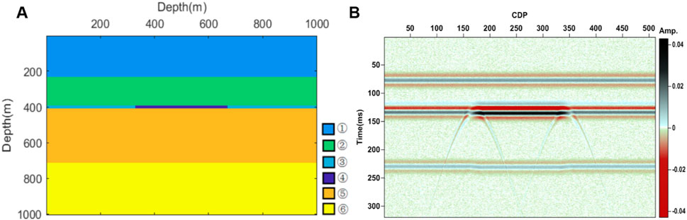
FIGURE 1. The geological model (A) and its corresponding seismic response with added Gaussian noise. SNR=15 dB (B).

TABLE 1

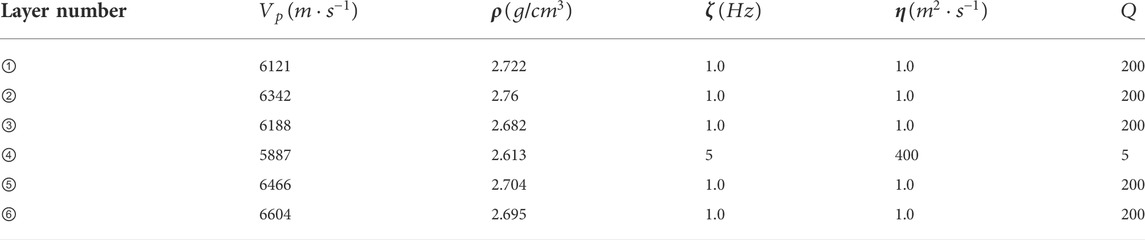
TABLE 1. Rock properties for the geological model. It is of note that ζ is the diffusion coefficient and η is the viscous coefficient.

Then, one seismic section (Figure 2) intersecting three known wells named A, B, and C, respectively, is collected from the Pugang gas field, China, for analysis. The gas field mainly contains carbonate reservoirs. The area between the two horizons is the main gas-producing reservoir. Wells A and B are prolific gas wells, and well C is a dry well. The seismic data is sampled at 2 ms.

FIGURE 2

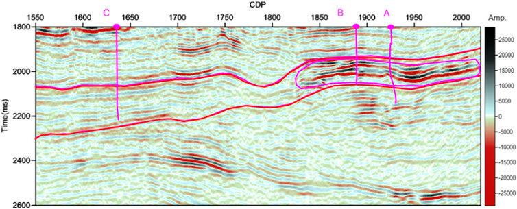
FIGURE 2. The seismic section intersecting three known wells, named A–C, respectively, from the Pugang gas field, China.

Multivariate variational mode decomposition

The purpose of MVMD is to extract several predefined multivariate modulated oscillations from the original multichannel signal. It is a constrained optimization problem (ur Rehman and Aftab, 2019):

$\begin{array}{l}\underset{\left\{u_{k,c}\right\},\left\{{\omega }_k\right\}}{\min }\left\{{\displaystyle \sum _k{\displaystyle \sum _c{\Vert {\partial }_t\left[u_{+}^{k,c}\left(t\right)e^{-j{\omega }_{k}t}\right]\Vert }_2^2}}\right\}\\ subjectto{\displaystyle \sum _k{u}_{k,c}}\left(t\right)=x_c\left(t\right).\left(c=\mathrm{1,2},\cdots ,C,k=\mathrm{1,2},\cdots ,K\right)\end{array}(1)$

where $C$ is the number of data channels and $K$ is the number of the predefined multivariate modulated oscillations, i.e., $x\left(t\right)={\displaystyle \sum _{k=1}^K{u}_k}\left(t\right)$, $u_k\left(t\right)=\left[u_1\left(t\right),u_2\left(t\right),\cdots ,u_C\left(t\right)\right]$, and $u_{+}^{k,c}\left(t\right)$ is the vector analytic representation of $u_{k,c}\left(t\right)$. Multivariate oscillations in $u_k\left(t\right)$ have a single common frequency component ${\omega }_k$ in all channels. To make (1) unconstrained, the following augmented Lagrangian function $L$ is used:

$\begin{array}{l}L\left(\left\{u_{k,c}\right\},\left\{{\omega }_k\right\},{\lambda }_c\right)=\alpha {{\displaystyle \sum _k{\displaystyle \sum _c\Vert {\partial }_t\left[u_{+}^{k,c}\left(t\right)e^{-j{\omega }_{k}t}\right]\Vert }}}_2^2\\ +{{\displaystyle \sum _c\Vert x_c\left(t\right)-{\displaystyle \sum _k{u}_{k,c}\left(t\right)}\Vert }}_2^2+{\displaystyle \sum _c\langle {\lambda }_c\left(t\right),x_c\left(t\right)-{\displaystyle \sum _k{u}_{k,c}\left(t\right)}\rangle },\end{array}(2)$

where $\lambda$ is the Lagrangian multiplier, and $\alpha$ is the balancing parameter of the data-fidelity constraint. The problem (Eq. 2) is solved using an alternate direction method of multipliers (ADMM) approach, which turns the whole optimization problem into several iterative sub-optimization problems. Then, the estimated modes and the center frequency are produced via the ADMM approach. The estimated modes in the frequency domain can be represented as

${\mathrm{u}}_{k,c}^{n+1}\left(\omega \right)=\frac{{\widehat{x}}_c\left(\omega \right)-{\displaystyle {\sum }_{i\ne k}{\widehat{u}}_{i,c}\left(\omega \right)+\frac{{\widehat{\lambda }}_c\left(\omega \right)}{2}}}{1+2\alpha {\left(\omega -{\omega }_k\right)}^2}.(3)$

The center frequency ${\omega }_k^{n+1}$ is updated as follows:

${\omega }_k^{n+1}=\frac{{\displaystyle \sum _c{\displaystyle {\int }_0^{\infty }\omega {\left|{\widehat{u}}_{k,c}\left(\omega \right)\right|}^{2}d\omega }}}{{\displaystyle \sum _c{\displaystyle {\int }_0^{\infty }{\left|{\widehat{u}}_{k,c}\left(\omega \right)\right|}^{2}d\omega }}}.(4)$

For all $\omega \ge 0$, the Lagrangian multiplier is updated by

${\widehat{\lambda }}_c^{n+1}\left(\omega \right)={\widehat{\lambda }}_c^n\left(\omega \right)+\tau \left({\widehat{x}}_c\left(\omega \right)-{\displaystyle \sum _k{\widehat{u}}_{k,c}^{n+1}\left(\omega \right)}\right),(5)$

until ${\displaystyle {\sum }_k{\displaystyle {\sum }_c\frac{{\Vert {\widehat{u}}_{k,c}^{n+1}-{\widehat{u}}_{k,c}^n\Vert }_2^2}{{\Vert {\widehat{u}}_{k,c}^n\Vert }_2^2}}}<\epsilon$.

A detailed description of the MVMD approach can be found in the study by ur Rehman and Aftab (2019).

Seismic attenuation estimation using MVMD

If only attenuation is considered, the amplitude of a plane wave in the time-frequency domain may be explicitly expressed as (Wang, 2004)

$S\left(t,\omega \right)=S_0\exp \left(-a\omega \right),(6)$

where $S_0$ is the amplitude at $t=0$, $S\left(t,\omega \right)$ is the amplitude at travel time $t$, and $\omega$ is the angular frequency. The absorption gradient or absorption coefficient $a$ is traditionally estimated through the slope of the logarithmic spectrum $\ln \left[S\left(t,\omega \right)/S_0\right]$ by using the high-frequency segment.

As shown by Eq. 6, the spectrum affected by absorption is a function of the form $\exp \left(-a\omega \right)$. The key of the absorption gradient estimation is to obtain the exponential attenuation coefficient of the signal spectrum.

The workflow of the proposed method is shown in Figure 3. For seismic data $s\left(t\right)$, we first use MVMD to decompose the seismic data into several IMFs. It is of note that if the number of some seismic traces is selected as a data channel, we need some adding zeros operation. Since each IMF is a monofrequency or narrow band signal, its spectrum is much smoother with narrow side lobes than that of the original seismic data, which facilitates a more accurate estimate than the conventional methods (Xue et al., 2014b; Xue et al., 2016b). Energy separation algorithm (ESA) using the Teager energy operator is proved to be more accurate in extracting the instantaneous attributes such as instantaneous amplitude (IA) and instantaneous frequency (IF) for monofrequency signals than the Hilbert transform (Maragos et al., 1993; Xue et al., 2014a). We then adopt ESA to extract the IA and IF of each IMF. The obtained IA and IF of each IMF can be expressed as (Maragos et al., 1993)

$\{\begin{array}{l}\left|a\left(n\right)\right|\approx 2{\psi }_d\left[u\left(n\right)\right]/\sqrt{{\psi }_d\left[u\left(n+1\right)-u\left(n-1\right)\right]}\\ \omega \left(n\right)\approx \arccos [1-{\psi }_d\left[u\left(n+1\right)-u\left(n-1\right)\right]/2{\psi }_d\left[u\left(n\right)\right]/2\end{array},(7)$

where ${\psi }_d(•)$ is a non-linear signal operator, ${\psi }_d\left[u\left(n\right)\right]=u^2\left(n\right)-u\left(n+1\right)u\left(n-1\right)$. Time-frequency spectrum is generated by the definition of a 3D space $\left[t,\omega \left(t\right),a\left(t\right)\right]$, where

$a\left(t\right)=H\left(\omega ,t\right)=\mathrm{Re}\left\{{\displaystyle \sum _{i=1}^k{a}_{c,i}\left(t\right)e^{i{\displaystyle \int {\omega }_{c,i}\left(t\right)dt}}}\right\}.(8)$

FIGURE 3

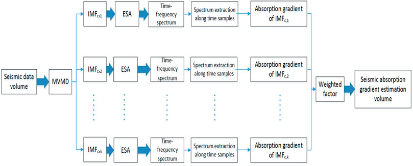
FIGURE 3. Workflow of the proposed method.

Next, we extract the amplitude spectrum along time samples for absorption gradient estimation for each IMF. We define the enhanced absorption gradient $a$ as follows:

$a=\left|a_{high}-a_{low}\right|,(9)$

where $a_{high}$ and $a_{low}$ are the slopes of curve fitting by applying the least squares method to the high-frequency segment and low-frequency segment of the logarithmic spectrum of each IMF, respectively. Figure 4 is an illustration of the curve fitting at the high-frequency segment and the low-frequency segment of a logarithmic spectrum. The Least squares fitting (LSF) is used here. It is of note that we use peak frequency as a reference to separate the spectrum into two parts. To better estimate the absorption gradient through a high-resolution time-frequency map, we take the difference scheme to estimate the absorption gradient at the low-frequency segment and the high-frequency segment of the logarithmic spectrum of an IMF with narrow band property. The low-frequency segment is selected as $[0.2E,0.8E]$, where $E$ denotes the energy of the low-frequency segment. The high-frequency segment is selected using the following expression:

$B\left(f\right)=\{\begin{array}{l}40,\left|f_{zr}-f_p\right|>40\\ \left(f_{zr}-f_p\right),\left|f_{zr}-f_p\right|<40\end{array},(10)$

where $f_{zr}$ is the first zero crossing frequency, and $f_p$ is the peak frequency.

FIGURE 4

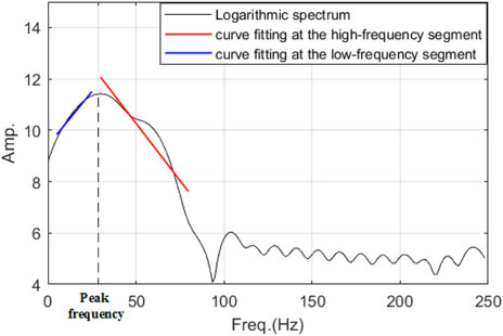
FIGURE 4. Curve fitting illustration.

A weighted IMF scheme with exponential decay characteristics which uses all IMFs with lower weight to undesirable IMFs instead of excluding them from the analysis entirely is evaluated to reflect more useful geologic information and yield high-resolution seismic reflection data (Macelloni et al., 2011; Xue et al., 2016b). Inspired by the weighted IMF scheme in the previous studies, when we obtain the enhanced absorption gradient for each IMF, we adopt a weighted factor $h$ for highlighting the contribution of each IMF:

$h=\{\begin{array}{l}1,\left|corr\left({\mathrm{u}}_{c,k},x_c\right)\right|\ge 0.5\\ 0.1,0.3\le \left|corr\left({\mathrm{u}}_{c,k},x_c\right)\right|<0.5\\ 0.01,0.1\le \left|corr\left({\mathrm{u}}_{c,k},x_c\right)\right|<0.3\\ 0.001,\left|corr\left({\mathrm{u}}_{c,k},x_c\right)\right|<0.1\end{array},(11)$

where $corr(•)$ denotes taking the correlation coefficient between $u_{c,k}$ and $x_c$. The final estimated absorption gradient $a$ of a seismic trace is the summarization of the weighted absorption gradient of each IMF:

$a_x={\displaystyle \sum _{k}h{a}_{u_{c,k}}}.(12)$

Results and analysis

Model test

Compared with the IMFs (Figures 5A and C) obtained by VMD, the IMFs (Figures 5B and D) obtained by MVMD show greater continuity in the lateral distribution, especially in the reservoir areas. It is of note that the IMFs obtained by VMD and MVMD are also different. IMF1 obtained by MVMD (Figure 5B) reflects more low-frequency features of the seismic response of the model, and more stratum and reservoir information are revealed in IMF2 obtained from MVMD (Figure 5D) than those from VMD (Figure 5C). It is clear that noise exists in both IMF1 and IMF2 of VMD. For comparison, we give the absorption gradient estimation using VMD applied to the high-frequency segment of the seismic bandwidth (Figure 6A) and the proposed method (Figure 6B). Both methods can detect the gas reservoirs, but the proposed method targets the gas reservoirs with more details highlighted.

FIGURE 5

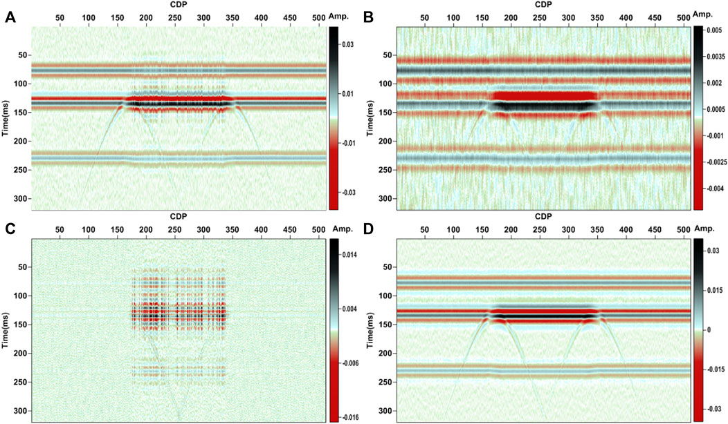
FIGURE 5. Model analysis. (A) IMF1 obtained by VMD. (B) IMF1 obtained by MVMD. (C) IMF2 obtained by VMD. (D) IMF2 obtained by MVMD. It is of note that for MVMD, the number of data channels is 6. The number of the predefined multivariate modulated oscillations for VMD and MVMD is 2. The moderate bandwidth constraint for VMD and MVMD is 200.

FIGURE 6

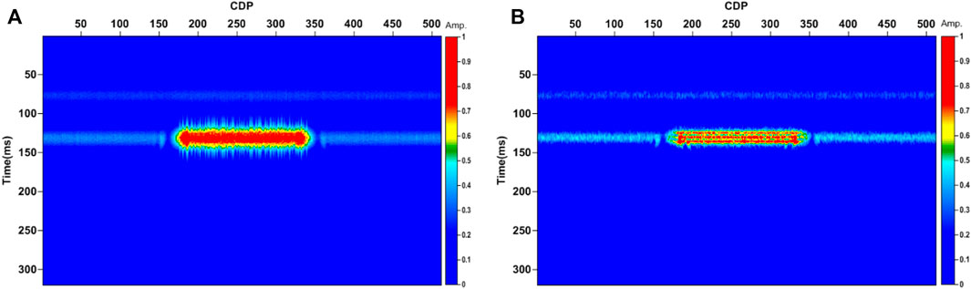
FIGURE 6. The absorption gradient section of the noisy data in Figure 1B estimated by (A) VMD and LSF applied at the high-frequency segment, and (B) the proposed method.

The model results show that the proposed method has a greater ability to give more accurate absorption gradient estimates. Furthermore, since the reservoir thickness and the wavelet frequency of the model are close to the actual reservoir thickness and the dominant frequency, the model results also suggest that the proposed method can be applied to the seismic data acquired in the Pugang gas field, China.

Field data analysis

IMFs obtained by the MVMD and the VMD are respectively shown in Figure 7. In Figure 7A–C, IMFs obtained by MVMD show more lateral continuities than those obtained by VMD (Figure 7D–F). Among IMFs obtained by MVMD, IMF1 shows more strata information; the gas reservoir shown by an irregular pink curve is highlighted in IMF2, while more details are reflected in IMF3. Stratum and fluid information are better reflected in different IMFs of MVMD than those of VMD.

FIGURE 7

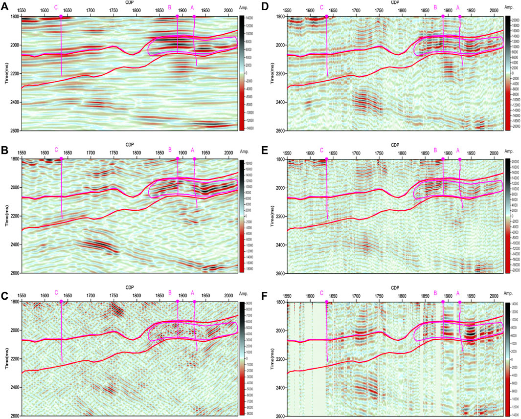
FIGURE 7. MFs of the seismic section. (A) IMF1 obtained by MVMD. (B) IMF2 obtained by MVMD. (C) IMF3 obtained by MVMD. (D) IMF1 obtained by VMD. (E) IMF2 obtained by VMD. (F) IMF3 obtained by VMD. It is of note that for MVMD, the number of data channels is set to 3. The number of the predefined multivariate modulated oscillations for VMD and MVMD is 3. The moderate bandwidth constraint for VMD and MVMD is 200.

Then, we applied the proposed method to the seismic section (Figure 2). Figure 8A shows the seismic section within the target layer. The absorption gradient section (Figure 8C) shows strong amplitude anomalies in the gas reservoirs where wells A and B are located, while there is no obvious amplitude anomaly in the area where dry well C locates. The proposed method gives a good gas-bearing interpretation with a high spatial and temporal resolution, which is more consistent with the results of the poststack wave impedance inversion section (Figure 8B).

FIGURE 8

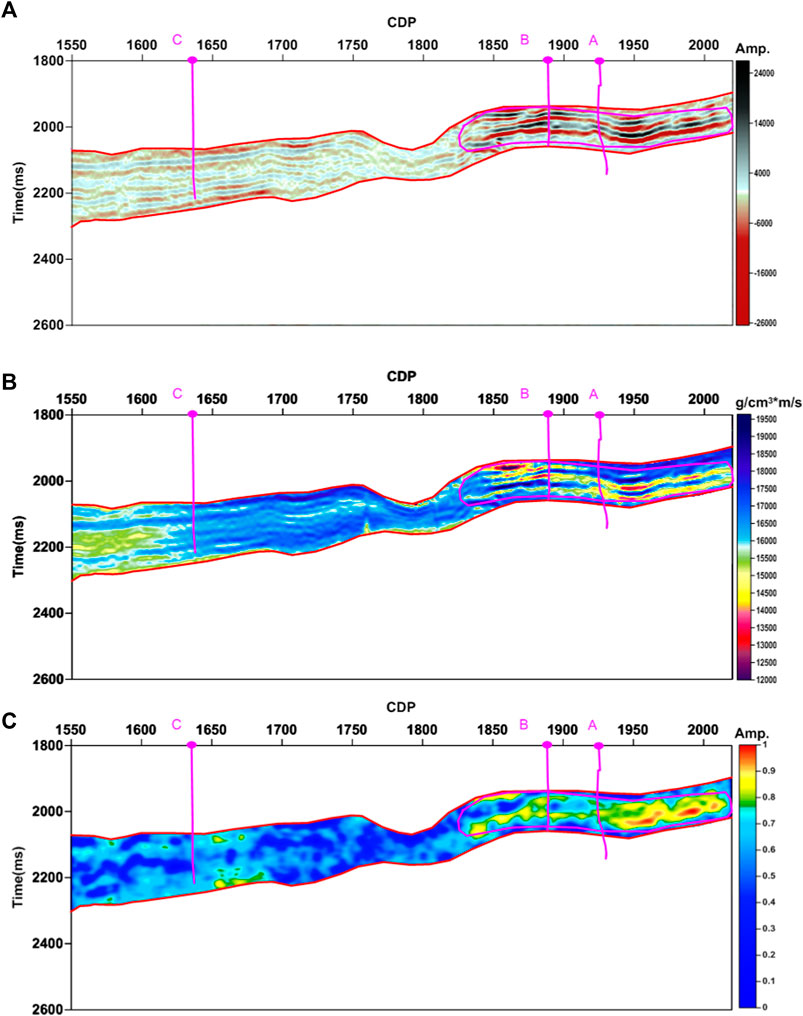
FIGURE 8. Results analysis. (A) The seismic section between the two horizons. (B) Poststack wave impedance inversion section. (C) The absorption gradient section using the proposed method. Only the seismic data between the two horizons are displayed.

Discussion

The influence of data channels selection for MVMD

Generally, seismic volume has a huge amount of seismic data. We cannot simply treat the whole number of seismic traces as a data channel used in MVMD due to the huge computing time; we need to select an appropriate data channel. Next, we investigate how the different data channels influence the features of the IMFs generated by MVMD.

We take the noisy data in Figure 1B as an example. Here, we use the correlation coefficient to measure the dependence between the two IMFs. A smaller correlation coefficient means the two modes can be considered to be quasi-orthogonal, and a larger correlation coefficient suggests two modes have a great correlation. Correlation coefficients computed from the IMFs with the different data channels (Table 2) show that a larger and nearly same (when the correlation coefficient retains the precision of two decimal places) correlation coefficient exists for the smaller data channels, and a very small correlation coefficient occurs for the larger data channels. We also can find that the smallest correlation coefficient exists for the case where the number of the whole seismic traces is used as the data channel. This fact suggests that if the number of all the seismic traces is used as the data channel, the IMFs generated by MVMD are quasi-orthogonal. But when the number of only some seismic traces is selected as a data channel, the different IMFs have a strong correlation. This may be caused by the fact that the adjacent seismic traces have some similar features and always change slowly in the stratigraphic characteristics. A smaller data channel cannot guarantee that the IMFs of the entire seismic volume are quasi-orthogonal. We give the IMFs sections with some different data channels in Figure 9. We can clearly find that the IMFs for channels 3, 9, and 200 are similar, and the first IMF (IMF1) has some similar features to the second IMF (IMF2). Noise information is more reflected in IMF1 than in IMF2 (Figures 9A, C, and E). Gas reservoir information is retrieved in both IMFs (Figure 9A–F). However, for channels 400 and 512, we can find that gas reservoir information is mainly reflected in IMF1 (Figures 9G and I), and the noise and some diffracted wave information are retrieved in IMF2 (Figures 9H and J). Figure 9 also illustrates that a strong correlation between the different IMFs exists for the case where the number of smaller seismic traces is selected as a data channel, and the quasi-orthogonal IMFs occur for the case when the number of comparatively larger seismic traces or the number of the whole seismic traces is selected as a data channel.

TABLE 2

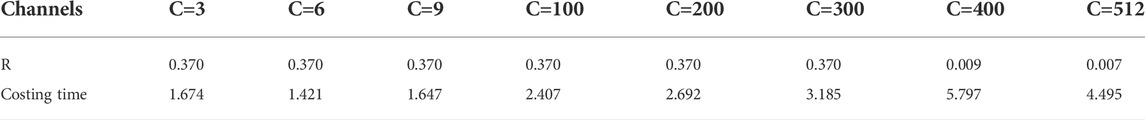
TABLE 2. Correlation and costing time analysis of the IMFs with the different channels for the noisy data in Figure 1B.

FIGURE 9

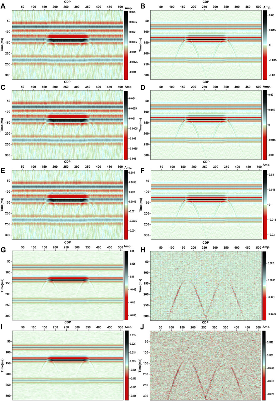
FIGURE 9. IMFs comparison of the different channels for the noisy data in Figure 1B. (A) IMF1 with channel 3. (B) IMF2 with channel 3. (C) IMF1 with channel 9. (D) IMF2 with channel 9. (E) IMF1 with channel 200. (F) IMF2 with channel 200. (G) IMF1 with channel 400. (H) IMF2 with channel 400. (I) IMF1 with channel 512. (J) IMF2 with channel 512.

But when we pay attention to the costing time of the different channels, we find that the costing time is mainly increased with the data channels if the number of some traces is selected as a data channel. Table 2 also shows that when the number of the whole seismic traces is selected as a data channel, the costing time is smaller than the case when the number of larger seismic traces is selected as the data channel. But the costing time for the case when the number of the whole seismic traces is selected as a data channel is still larger than those taking the number of smaller traces as data channels.

Figure 10 shows how the IMFs of the different channels influence the resulted absorption gradient section using the proposed method. It is clearly seen that regardless of the number of channels selected, the final attenuation gradient estimation sections can all well-target the gas reservoir. However, there are also some minor differences. When the data channel is 3 or 6, the absorption gradient section reveals more details of the gas reservoirs, while when the data channel is 400 or 512, upper and lower reflection surfaces are more highlighted.

FIGURE 10

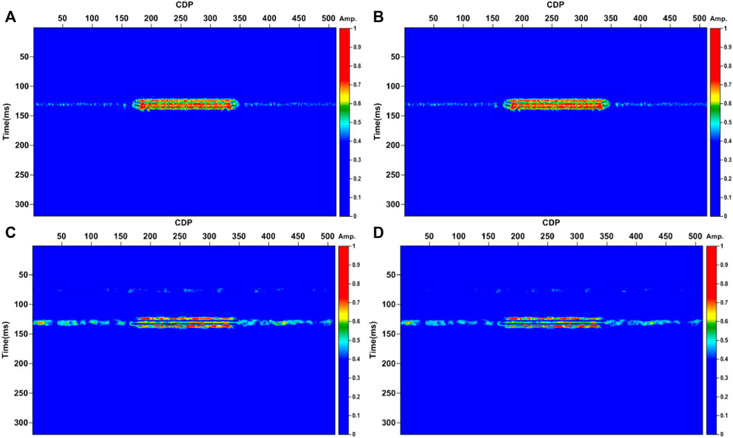
FIGURE 10. The absorption gradient section of the different channels using the proposed method for the noisy data in Figure 1B. (A) With channels of 3. (B) With channels of 6. (C) With channels of 400. (D) With channels of 512.

Therefore, for seismic data, when we estimate the attenuation gradient, considering the costing time and attenuation estimation results, we can choose a smaller number as a data channel for MVMD.

The comparison of the attenuation gradient estimation using the different methods

Here, we take the seismic section in Figure 8A for comparison of the attenuation gradient estimation using the different methods. The conventional absorption gradient method adopted CWT with the two-point slope estimation (Figure 11A) gives the poorest interpretation. Figure 11A shows slightly stronger amplitude anomalies in the area where wells A and B locate, but the strongest amplitude anomalies are found in the area where dry well C locates. The conventional absorption gradient method adopted CWT with LSF (Figure 11C) improves the interpretation of the gradient method using CWT and the two-point slope estimation. However, the detected amplitude anomalies in the area where wells A and B locate are not consistent with the gas test results. The absorption gradient estimation using VMD and LSF (Figure 11B) at the high-frequency segment greatly improves the interpretation results than those conventional methods. But when compared with the proposed method, it gives a poorer spatial and temporal resolution. The proposed method (Figure 11D) gives the best gas-bearing interpretation in the area where wells A and B are located, which is more consistent with the results of the poststack wave impedance inversion section.

FIGURE 11

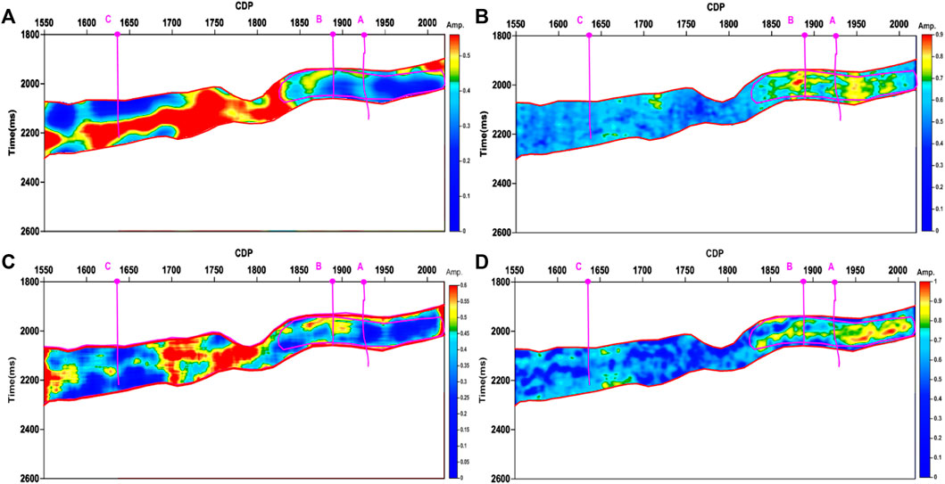
FIGURE 11. The absorption gradient sections using the different methods. (A) The conventional absorption gradient section using the continues WT (CWT) and the two-point slope estimation. (B) The absorption gradient section using VMD and LSF at a high-frequency band. (C) The conventional absorption gradient section using CWT and LSF at a high-frequency band. (D) The absorption gradient section using the proposed method. Only the seismic data between the two horizons are displayed.

Prospect on future work

From the model analysis (Figure 6) and the field data applications results (Figures 8 and 11), we can find that the MVMD-based seismic attenuation estimation method can give higher spatial and temporal results and yield better gas-bearing interpretations when compared with the conventional absorption gradient estimation methods and the VMD-based absorption gradient estimation method. The advantages of the MVMD-based seismic attenuation estimation method are mainly based on the following key steps. First, IMFs from MVMD make some seismic attenuation information in certain frequency bands highlighted with great lateral continuity. Second, we use the Teager energy separation algorithm to generate the time-frequency spectrum with a high resolution for each IMF. The usage of the low-frequency and high-frequency segments of the amplitude spectrum extracted from the time-frequency map further improves the accuracy of the absorption gradient estimates. Third, we adopt the weighted factor shown in Eq. 11 for highlighting the different attenuation contributions of each IMF.

Although the MVMD-based seismic attenuation estimation method has more advantages than the conventional methods and VMD-based method, we still need to pay attention to the fact that the selection of data channels in the proposed method will affect the processing speed and the attenuation results. Otherwise, we need to choose the number of data channels reasonably according to the actual data characteristics. A smaller number as a data channel for MVMD is suggested for huge seismic data processing. The number of the predefined multivariate modulated oscillations for MVMD should also be properly selected for hydrocarbon detection. In practice, a commonly used way to select the predefined multivariate modulated oscillations for MVMD is having several trials to choose the suitable predefined number (usually in the range of two to four) to obtain the optimal performance. In addition, although we have given the selection criteria for the low-frequency and high-frequency ranges for different actual regional seismic data, the frequency range selection still needs to be slightly adjusted according to the actual situation.

The proposed seismic attenuation estimation method using MVMD can be used for detecting the presence of fluids in reservoir characterization. Further study of the proposed method in other study areas will enhance the understanding of the practical restrictions and advantages of this approach.

Conclusion

We presented a seismic attenuation estimation method using MVMD. MVMD obtains the local average value by obtaining signal projections in different directions in the n-dimensional space, which is more conducive to obtaining the lateral change characteristics of seismic signals while capturing reservoir information. IMFs obtained by MVMD have more lateral continuities than those obtained by VMD. Stratum and fluid information are better reflected in different IMFs of MVMD than those of VMD. The absorption gradient using the low-frequency segment combined with the high-frequency segment of the spectrum of each IMF can improve the accuracy of the absorption gradient estimation. Model test and field data examples show the proposed method can better target the gas reservoirs with high spatial and temporal resolution than the traditional methods and the VMD-based method.

Data availability statement

The raw data supporting the conclusions of this article will be made available by the authors, without undue reservation.

Author contributions

J-ZL: writing—original draft, modeling, programming, and interpretation. Y-jX: writing—review and editing, validation, and interpretation. LS: writing—review and editing, data preparation, and validation. LH: supervision, writing—review and editing, and interpretation.

Funding

This work is supported in part by the Central Government Funds of Guiding Local Scientific and Technological Development for Sichuan Province under Grant 2021ZYD0030 and in part by the open Fund of Sinopec Petroleum Exploration and Production Technology Research Institute under Grant GSYKY-B09-32.

Conflict of interest

The authors declare that the research was conducted in the absence of any commercial or financial relationships that could be construed as a potential conflict of interest.

Publisher’s note

All claims expressed in this article are solely those of the authors and do not necessarily represent those of their affiliated organizations, or those of the publisher, the editors, and the reviewers. Any product that may be evaluated in this article, or claim that may be made by its manufacturer, is not guaranteed or endorsed by the publisher.

References

Anderson, A. L., and Hampton, L. D. (1980). Acoustics of gas-bearing sediments I. Background. J. Acoust. Soc. Am. 67 (6), 1865–1889. doi:10.1007/s12583-011-0163-z

CrossRef Full Text | Google Scholar

Chen, X. H., He, Z. H., and Zhong, W. L. (2011). Numeric simulation in the relationship between low frequency shadow and reservoir characteristic. J. China Univ. Min. Technol. 40 (4), 584–591. in Chinese. doi:10.1121/1.384453

CrossRef Full Text | Google Scholar

del Valle-García, R., and Ramírez-Cruz, L. (2002). Spectral attributes for attenuation analysis in a fractured carbonate reservoir. Lead. Edge 21 (10), 1038–1041. doi:10.1190/1.1518443

CrossRef Full Text | Google Scholar

Dragomiretskiy, K., and Zosso, D. (2014). Variational mode decomposition. IEEE Trans. Signal Process. 62 (3), 531–544. doi:10.1109/tsp.2013.2288675

CrossRef Full Text | Google Scholar

Duchesne, M. J., Halliday, E. J., and Barrie, J. V. (2011). Analyzing seismic imagery in the time–amplitude and time–frequency domains to determine fluid nature and migration pathways: a case study from the queen charlotte basin, offshore British Columbia. J. Appl. Geophys. 73 (2), 111–120. doi:10.1016/j.jappgeo.2010.12.002

CrossRef Full Text | Google Scholar

Dvorkin, J., and Nur, A. (1993). Dynamic poroelasticity: a unified model with the squirt and the biot mechanisms. Geophysics 58 (4), 524–533. doi:10.1190/1.1443435

CrossRef Full Text | Google Scholar

Gabor, D. (1946). Theory of communication. J. Institution Electr. Eng. 93 (26), 429–457.

CrossRef Full Text | Google Scholar

Huang, N. E., Shen, Z., Long, S. R., Wu, M. C., Shih, H. H., Zheng, Q., et al. (1998). The empirical mode decomposition and the Hilbert spectrum for nonlinear and non-stationary time series analysis. Proc. R. Soc. Lond. A 454, 903–995. doi:10.1098/rspa.1998.0193

CrossRef Full Text | Google Scholar

Korneev, V. A., Goloshubin, G. M., Daley, T. M., and Silin, D. B. (2004). Seismic low-frequency effects in monitoring fluid-saturated reservoirs. Geophysics 69 (2), 522–532. doi:10.1190/1.1707072

CrossRef Full Text | Google Scholar

Liu, N., Zhang, B., Gao, J., Gao, Z., and Li, S. (2018). Seismic attenuation estimation using the modified log spectral ratio method. J. Appl. Geophys. 159, 386–394. doi:10.1016/j.jappgeo.2018.09.014

CrossRef Full Text | Google Scholar

Liu, N., Zhang, B., Gao, J., Wu, H., and Li, S. (2019). Seismic anelastic attenuation estimation using prestack seismic gathers. Geophysics 84 (6), M37–M49. doi:10.1190/geo2017-0811.1

CrossRef Full Text | Google Scholar

Lou, Y., Zhang, H., Liu, N., Liu, R., and Sun, F. (2021). Multi-scale coherence attribute and its application on seismic discontinuity description. IEEE Geosci. Remote Sens. Lett. 19, 3004705. doi:10.1109/lgrs.2021.3132358

CrossRef Full Text | Google Scholar

Macelloni, L., Battista, B. M., and Knapp, C. C. (2011). Optimal filtering high-resolution seismic reflection data using a weighted-mode empirical mode decomposition operator. J. Appl. Geophys. 75, 603–614. doi:10.1016/j.jappgeo.2011.09.018

CrossRef Full Text | Google Scholar

Maragos, P., Kaiser, J. F., and Quatieri, T. F. (1993). On amplitude and frequency demodulation using energy operators. IEEE Trans. Signal Process. 41 (4), 1532–1550. doi:10.1109/78.212729

CrossRef Full Text | Google Scholar

Martín, N. W., Azavache, A., and Donati, M. S. (1998). “Indirect oil detection by using P-wave attenuation analysis in Eastern Venezuela Basin,”. SEG Technical Program Expanded Abstracts 1998 in 1998 SEG annual meeting, New Orleans, Louisiana, September 13–18, 1998, 914–917.

Google Scholar

Mitchell, J. T., Derzhi, N., Lichman, E., and Lanning, E. N. (1996). “Energy absorption analysis: a case study,”. SEG Technical Program Expanded Abstracts 1996 in 1996 SEG annual meeting, Denver, Colorado, November 10–15, 1996, 1785–1788.

CrossRef Full Text | Google Scholar

Müller, T. M., Gurevich, B., and Lebedev, M. (2010). Seismic wave attenuation and dispersion resulting from wave-induced flow in porous rocks—a review. Geophysics 75 (5), 75A147–75A164. doi:10.1190/1.3463417

CrossRef Full Text | Google Scholar

Reine, C., Clark, R., and van der Baan, M. (2012). Robust prestack Q-determination using surface seismic data: Part 1—method and synthetic examples. Geophysics 77 (1), R45–R56. doi:10.1190/geo2011-0073.1

CrossRef Full Text | Google Scholar

Torres, M. E., Colominas, M. A., Schlotthauer, G., and Flandrin, P. (2011). “A complete ensemble empirical mode decomposition with adaptive noise,” in 2011 IEEE international conference on acoustics, speech and signal processing (ICASSP), Prague, Czech Republic, 22-27 May 2011, 4144–4147.

CrossRef Full Text | Google Scholar

ur Rehman, N., and Aftab, H. (2019). Multivariate variational mode decomposition. IEEE Trans. Signal Process. 67 (23), 6039–6052. doi:10.1109/tsp.2019.2951223

CrossRef Full Text | Google Scholar

Wang, Y. (2004). Q analysis on reflection seismic data. Geophys. Res. Lett. 31 (17), L17606. doi:10.1029/2004gl020572

CrossRef Full Text | Google Scholar

Xiong, X. J., He, X. L., Pu, Y., He, Z. H., and Lin, K. (2011). High-precision frequency attenuation analysis and its application. Appl. Geophys. 8 (4), 337–343. doi:10.1007/s11770-011-0302-4

CrossRef Full Text | Google Scholar

Xue, Y.-j., Cao, J.-x., and Tian, R.-f. (2013). A comparative study on hydrocarbon detection using three EMD-based time-frequency analysis methods. J. Applied Geophys. 89, 108–115.

CrossRef Full Text | Google Scholar

Xue, Y-J., Cao, J-X., and Tian, R-F. (2014a). EMD and Teager–Kaiser energy applied to hydrocarbon detection in a carbonate reservoir. Geophys. J. Int. 197 (1), 277–291. doi:10.1093/gji/ggt530

CrossRef Full Text | Google Scholar

Xue, Y. J., Cao, J. X., Du, H. K., Lin, K., and Yao, Y. (2016a). Seismic attenuation estimation using a complete ensemble empirical mode decomposition-based method. Mar. Pet. Geol. 71, 296–309. doi:10.1016/j.marpetgeo.2016.01.011

CrossRef Full Text | Google Scholar

Xue, Y. J., Cao, J. X., Du, H. K., Zhang, G. L., and Yao, Y. (2016b). Does mode mixing matter in EMD-based highlight volume methods for hydrocarbon detection? Experimental evidence. J. Appl. Geophys. 132, 193–210. doi:10.1016/j.jappgeo.2016.07.017

CrossRef Full Text | Google Scholar

Xue, Y. J., Cao, J. X., Tian, R. F., Du, H. K., and Shu, Y. X. (2014b). Application of the empirical mode decomposition and wavelet transform to seismic reflection frequency attenuation analysis. J. Petroleum Sci. Eng. 122, 360–370. doi:10.1016/j.petrol.2014.07.031

CrossRef Full Text | Google Scholar

Zhang, Y., Zhang, H., Yang, Y., Liu, N., and Gao, J. (2021). Seismic random noise separation and attenuation based on MVMD and MSSA. IEEE Trans. Geosci. Remote Sens. 60, 1–16. doi:10.1109/tgrs.2021.3131655

CrossRef Full Text | Google Scholar