Hidden molecular clues in marine sediments revealed by untargeted mass spectrometry imaging

1 Introduction

Biomarkers in geological samples encode information about past environments and ecosystems (Hayes et al., 1990; Peters et al., 2005). Biomarker-based molecular proxies have been widely applied in reconstructing paleoecological and paleoclimatic history (Damsté et al., 1990; Hinrichs et al., 1999; Huang et al., 1999; Summons et al., 2022). The initial proposal of molecular stratigraphy occurred more than three decades ago (Brassell et al., 1986), when the degree of unsaturation of long-chain methyl and ethyl ketones (i.e., alkenones) produced by ubiquitous coccolithophores was suggested to indicate variations in sea surface temperatures (SST). Another example of a biomarker-based proxy is the stanol/stenol ratio, which is sensitive to redox conditions in depositional settings (Nishimura and Koyama, 1977; Wakeham, 1989) as ${\mathrm{\Delta }}^5$-sterols are microbiologically reduced to $5\alpha$ (H)-stanols under anoxic conditions (Rosenfeld and Hellman, 1971; Eyssen et al., 1973). Conventional biomarker analysis includes the solvent extraction of geological samples, the subsequent separation of the extract into varying fractions, and the instrumental analysis of the crude extract or selected fractions. Due to the requirement of at least gram-sized (cm-scale) sample amounts in such analytical protocols, the resulting biomarker records usually indicate the average state of past environments and ecosystems over decades to millennia and are not fine enough for identifying abrupt environmental changes and high-frequency climate oscillations.

Recently, we have increased the resolution of biomarker records in sediments to μm-scale by an extraction-free, mass spectrometry imaging (MSI)-based approach via matrix-assisted laser desorption/ionization coupled to Fourier transformation-ion cyclotron resonance-mass spectrometry (MALDI-FT-ICR-MS; Wörmer et al., 2014, Wörmer et al., 2019; Alfken et al., 2019). In the annually varved sediment of the Santa Barbara Basin (SBB), such a fine resolution allows deciphering sub-annual distributions of archaeal tetraether lipids, haptophyte-derived alkenones, and sterols, which are sensitive to changes in upwelling intensity, sea surface temperature, and water column redox conditions (Alfken et al., 2020, 2021). The MSI-based protocol has also successfully revealed astonishingly diverse spatial signatures of lipid biomarkers along a ∼1 cm thick microbial mat (Wörmer et al., 2020), demonstrating its capability in resolving fine spatial distributions of biomarker records beyond rather coarse concentration profiles. Nevertheless, our MSI-based studies of sedimentary archives so far have only focused on certain groups of biomarkers, such as alkenones and sterols. Thousands of ions are generated in a single spectrum of each μm-sized laser spot in addition to these targeted biomarkers, resulting in massive amounts of spectrometry data that are not readily mineable but could contain novel, biogeochemically relevant biomarkers. An untargeted data processing protocol is thus in need for the comprehensive understanding of sedimentary MSI datasets.

Over the last decade, advances in bioinformatics have shed light on hidden molecular clues in MSI datasets obtained from biological tissues, providing automated tools/protocols for data cleaning, as well as unsupervised and supervised data mining (reviews in Alexandrov, 2012; Trede et al., 2012; Thiele et al., 2014; Verbeeck et al., 2020). For example, Eriksson et al. (2019) proposed a sensitive peak detection method based on cluster-wise kernel density estimation (KDE), an algorithm for estimating the probability density function of random variables (Botev et al., 2010), allowing the discovery of both faint and localized peaks in MSI datasets. Gray level co-occurrence matrices (GLCM; Hall-Beyer, 2017) that compute the distribution of co-occurring pixel values at specified offsets in an image were utilized in Wijetunge et al. (2015) for unsupervised peak picking, which enables identifying molecules with structured spatial distributions. Various matrix factorization techniques, such as principal component analysis (PCA; Jolliffe, 2002), independent component analysis (ICA; Jutten and Herault, 1991; Comon, 1994), and non-negative matrix factorization (NMF; Brunet et al., 2004; Kim and Park, 2007) have been successfully applied to MSI datasets for dimensionality reduction and feature extraction. Among these, NMF is specifically useful in extracting easy-to-interpret biologically relevant information (e.g., Siy et al., 2008; Gut et al., 2015; Nijs et al., 2021). In addition to these unsupervised approaches, supervised machine learning has also been reported for identifying tumor tissues and discovering tumor-related biomarkers (e.g., Quanico et al., 2017; Ovchinnikova et al., 2020; Mittal et al., 2021).

Data mining approaches designed for biological MSI datasets often take advantage of the spatial resolution of MSI and search for biomarkers that co-localize with specific biological structures, e.g., tumors. Although geological samples are generally not as clearly structured as biological tissues, the laminated samples from the Santa Barbara Basin should be imprinted with distinct spatial molecular signatures caused by seasonally recurring biogeochemical processes. For instance, sediments in the center of SBB are deposited in oxygen-depleted settings, and they are characterized by annual varve couplets of terrigenous mineral-rich laminae deposited during the rainy fall–winter season alternating with biogenic-rich laminae deposited during the highly productive spring–summer season (Hülsemann and Emery, 1961; Reimers et al., 1990; Thunell et al., 1995; Schimmelmann and Lange, 1996). Such distinct sources should be reflected in biomarker signatures that are, to some extent, correlated with environmental conditions, such as salinity and nutrient concentrations.

In this study, we reported an untargeted data processing workflow for dissecting sedimentary MSI datasets and extracting information beyond conventional molecular proxies, enabling us to discover unique molecular signatures imprinted by varying biogeochemical processes in sediments. The proposed workflow is validated by re-analyzing the MSI datasets obtained from the SBB sediments measured by Alfken et al. (2020, 2021). Untargeted peak detection, selection of informative peaks whose distributions mirror the lamination of the sediment, pattern recognition for molecular signature discovery, and relating molecular signatures to environmental variables are all part of the re-analysis. In addition, conventional molecular proxies are often established in a bottom-up manner, starting at characterizing specific biomarkers in geological samples, then identifying their roles in biogeochemical processes, and, in the end, building geochemically meaningful proxies that stand the test of “time” and “space”. In this study, based on the proposed data processing workflow, we tried to demonstrate the potential of supervised learning for discovering novel, biogeochemically relevant molecular proxies in a top-down manner, i.e., building indicative proxies without prior knowledge of their biogeochemical implications.

2 Samples and methods

2.1 Mass spectrometry imaging experiments and datasets

Four MSI datasets (Table 1) acquired from the uppermost ∼10 cm of box core SPR0901-05BC collected from the center of SBB were employed to evaluate the data processing workflow proposed in this study. The sediment samples and MALDI-FT-ICR-MS analysis protocol have been described in detail in Alfken et al. (2020, 2021). Datasets A1 and A2 were measured in Alfken et al. (2020) with a mass window of 520–580 Da for mapping the $U_{37}^{K^{\prime }}$ index, and datasets B1 and B2 were measured in Alfken et al. (2021) with a wider mass window of 375–525 Da for mapping the stanol/stenol ratios. A1 and B1 were obtained from the uppermost ∼5 cm of the sediment, and A2 and B2 were obtained from 5–10 cm intervals on the sediment. For the sake of brevity, A1 and A2, and B1 and B2 were merged, respectively, in this study, and the resulting new datasets were coded as datasets A and B. In addition, although datasets resulting from analysis of the m/z range 1280–1360 are available from Alfken et al. (2021), they were deemed not to be practical for evaluating the untargeted workflow due to the low abundance of known biomarkers in this mass range.

TABLE 1

TABLE 1. Basic information of the MSI datasets employed in this study.

2.2 Data processing workflow

The MSI datasets were first exported to plain text files (*.txt) from Data Analysis version 4.4 software (Bruker Daltonics). These plain text files were taken as inputs by the proposed workflow (Figure 1) in this study, which is implemented in an in-house developed python package that is publicly available (https://github.com/weimin-liu/msi_feature_extraction). In brief, the workflow includes a data cleaning module for mass calibration, peak normalization, peak alignment, and peak picking, and a data mining module for molecular signature extraction and clustering of molecules. In addition, ElasticNet was employed to train multivariate linear regression models for indicating environmental conditions using the data mining results, in order to demonstrate the potential of supervised learning for molecular proxy discovery. The individual steps and the rationale of the proposed workflow are described in detail in the following sections.

FIGURE 1

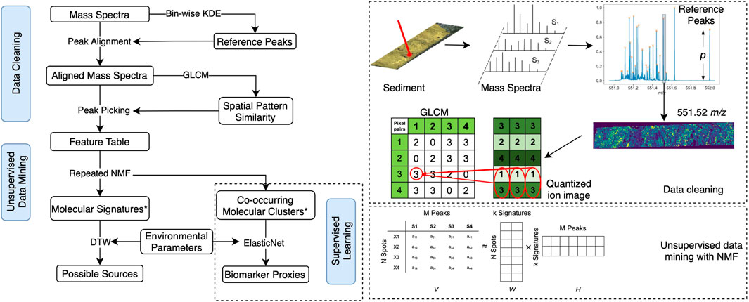
FIGURE 1. (A) Proposed workflow including data cleaning and data mining modules for the untargeted analysis of the sedimentary MSI dataset, supplemented by a supervised learning example to demonstrate its potential for the discovery of novel biomarker proxies on the basis of the proposed workflow. * Molecular signatures refer to the small sets of hidden features extracted by repeated NMF, and they denote the commonality of co-occurring molecules. By contrast, ElasticNet tries to find the variability in these co-occurring molecules that correlate with certain environmental parameters. (B) Graph shows an example of the workflow, including the detection of reference peaks between m/z values 551.0 and 552.0, the calculation of the gray level co-occurrence matrix (GLCM), and the unsupervised data mining with non-negative matrix factorization (NMF).

2.2.1 Data cleaning

In this step, the spectra were first calibrated, normalized by median peak intensity, aligned onto common mass-to-charge (m/z) ratios detected by bin-wise KDE, and cleaned by a two-step peak picking method to extract robust and informative signals in the spectra, including a peak prominence filter and a geochemical-context-based filter based on the varying deposits visualized by the X-Ray image of the sediment.

2.2.1.1 Mass calibration and peak intensity normalization

Raw spectra were calibrated with lock-mass calibration in data analysis before being exported (Alfken et al., 2020, 2021). Subsequently, a quadratic mass error function was fitted from the mass deviations of calibrants in each spectrum for further calibration. The calibrants used in datasets A and B are listed in Supplementary Table S1. They were the most ubiquitous compounds in each dataset whose chemical formulas can be assigned with great certainty. In addition, peak intensities in each spectrum were normalized to the median peak intensity of the spectrum as it was found to be robust against artifact generation such as ion images showing inaccurate ion distributions (Deininger et al., 2011; Fonville et al., 2012).

2.2.1.2 Peak alignment with bin-wise KDE and peak prominence filtering

For a molecule whose theoretical m/z is $m{z}_i$, its measured m/z in the spectrum $S_j$ is $m{z}_{i,j}$ that has a random deviation from $m{z}_i$. We assume $m{z}_{i,j}$ is normally distributed around $m{z}_i$ and determined $m{z}_i$ from the distribution of $m{z}_{i,j}$ with KDE. The so-determined $m{z}_i$ ratios are referred to as reference m/z ratios in this study since they do not necessarily represent the exact theoretical m/z ratios.

Concretely, we adapted the cluster-wise KDE approach proposed in Eriksson et al. (2019) by omitting peak clustering and detecting peaks directly in mass bins. We used mass bins with an interval of 1 Da starting at every integer mass (e.g., 375.0—376.0 Da) to collect m/z from all spectra and got an array of bins [$bi{n}_1$, $bi{n}_2$, $bi{n}_3$, …]. We then fitted KDE to the distribution of m/z within each sorted bin using a Gaussian kernel function, the bandwidth of which is automatically selected by the improved Sheather Jones algorithm implemented in the python package KDEpy (Odland, 2018), which is robust in fitting multimodal distributions (Botev et al., 2010). Reference m/z ratios were detected on the KDE curve by first normalizing its height to [0, 1] and then picking local maxima with peak prominence (defined in Virtanen et al., 2020) greater than a pre-defined threshold p_th (p_th $\in$ (0, 1)). How the choice of p_th influences the peak picking results, including the quality and the coverage of resulting peaks, is evaluated in Supplementary Text S1. Finally, all spectra were aligned onto the reference m/z ratios by picking the nearest neighbor (i.e., the closest peak) with a maximum drift threshold of 10 ppm.

2.2.1.3 Peak picking with GLCM features: Geochemical-context-based peak picking

The reference peaks detected by bin-wise KDE likely contained signals of background noise and non-informative peaks that cannot be reliably removed by peak prominence filtering. In this study, we defined informative peaks as those having certain spatial structures instead of being randomly distributed in the sediments. The two datasets were obtained from the varved SBB sediments consisting of seasonally alternating deposits, which allow the visualization of the associated density differences on an X-ray image (positive image). Since the dense, terrestrial deposits are displayed as dark, and the more porous, diatom-rich biogenic deposits as light laminae (Hülsemann and Emery, 1961; Soutar and Crill, 1977; Reimers et al., 1990; Thunell et al., 1995), it is reasonable to assume that geochemically informative peaks should inherit similar spatial patterns. Based on this assumption, a geochemical-context-based peak picking method was employed in the workflow as a supplementary approach to peak prominence filtering.

Concretely, ion images were first generated using normalized ion intensity maps across the sediment slide and were then preprocessed using a similar approach, as described in Wijetunge et al. (2015). In brief, each ion image was first rescaled to include all intensities that fall between the 2nd and 98th percentiles to remove hotpots and was subsequently smoothed by a mean filter with a 3 $\times$ 3 neighborhood (raster) to reduce technical artifacts. All intensity values excluding 0 in each image were then quantized to 11 integer intensity levels based on the respective intensity histogram. The resulting ion images had 12 shades of gray, in which 0 denotes the absence of the peak, while 1—11 denote increasing peak intensities. The X-ray photograph of the uppermost ∼10 cm sediment slide exhibits the characteristic varved structure of SBB sediments, and it was thus targeted for spatial similarity comparison. Instead of computing pixel-to-pixel correlations or the GLCM scores proposed in Wijetunge et al. (2015), the features extracted using GLCM from the ion images and X-ray photographs were compared (Haralick et al., 1973). We used the approach implemented in the python package scikit-image (van der Walt et al., 2014) to calculate GLCM features, including contrast, dissimilarity, correlation, energy, and homogeneity, for the quantized ion images and X-ray photographs in 0°, 15°, 45°, 90°, 105°, 135°, and 270° angles, with pixel pair distance offsets from 1—5. The output for each image was a 175-dimension GLCM feature vector. Principal component analysis (PCA) was performed on the standardized GLCM feature vectors to visualize their variability in GLCM features. The cosine similarities between the GLCM feature vector of ion images and those of X-ray photographs were computed for ranking the ion images, and the cutoff for peak picking was determined by manually examining every fifth percentile of the ranked ion images.

2.2.2 Data mining with NMF

2.2.2.1 Spatial molecular signatures discovered with repeated NMF

The MSI dataset $V$ after data cleaning is a $m \times n$ matrix that has $m$ spectra, each of which has $n$ peaks. We assume molecules that are produced by the same living organisms or related to the same biogeochemical processes should have similar spatial distribution patterns (signatures) in the sediments. Mathematically, assuming $V$ has a total of k unique signatures, we can discover a matrix $W$ that denotes these spatial signatures and a matrix $H$ that denotes the associated molecule clusters, given the factorization $V\sim WH$ (Brunet et al., 2004). The resulting matrices $W$ and $H$ have a dimension of $m \times k$ and $k \times n$, respectively, and both contain only non-negative entries (i.e., NMF). The NMF algorithm implemented in the python package scikit-learn (Pedregosa et al., 2011) was employed in this study.

Since NMF does not necessarily converge to the same solution over multiple runs, its rank $k$, i.e., the number of clusters/signatures, needs to be properly estimated in order to get the most stable results. Therefore, we factorized $V$ 30 times with random initial conditions at each rank between 3—20 and computed the corresponding consensus matrix $\bar{\mathrm{C}}$, following the approach described in Brunet et al. (2004). The stability of $\bar{\mathrm{C}}$ denotes how strong the clustering of $V$ into k classes is and can be measured by the cophenetic correlation coefficient (Brunet et al., 2004) and dispersion coefficient (Kim and Park, 2007), in both of which 1 denotes the most stable clustering, while 0 denotes the least stable clustering. In addition, given the apparent fact that sedimentary MSI datasets are not as well-structured as datasets obtained from biological tissues, similar $W$ and $H$ derived over multiple NMF runs were accumulated to highlight the stable signatures. In other words, for the $i_{th}$ spatial signature discovered in the $j_{th}$ NMF runs $W_{i,j}$ and $H_{i,j}$, if they were strongly correlated (Pearson’s r > 0.9) with signatures $W_{m,n}$ and $H_{m,n}$ ($n<j)$ discovered in previous NMF runs, $W_{i,j}$ and $H_{i,j}$ were, respectively, added onto $W_{m,n}$ and $H_{m,n}$.

In addition, a co-occurrence molecular network was constructed based on the consensus matrix C̄. Nodes in the network represent the column and row indices in C̄, and the thickness of edges between the nodes denotes the corresponding entries in C̄.

2.2.2.2 Linking quarterly averaged signatures with environmental parameters

Each obtained signature is a matrix that has the same dimension as the ion images in the spectra, and its entry $w_{i,j}$ denotes the abundance (median normalized peak intensity) of the signature at the location $(i, j)$ on the sediment slide. In this step, in order to find the geochemical implications and the potential drivers of these mathematically derived signatures, we converted them to quarterly averaged time series using the same approach described in Alfken et al. (2021), including correcting tilted laminae, and transforming the spot coordinates to depth and age using the tie points of the age model. The age model of SPR0901-05BC was established by varve counting and additional identification of specific marker layers on the basis of the X-ray image, yielding an accuracy of ±1 year for the data reported in this study (Schimmelmann & Lange, 1996). The resulting temporal sequences were compared with seasonally measured water column data, including temperature, salinity, oxygen concentrations, and nutrient concentrations, at the CalCOFI (California Cooperative Oceanic Fisheries Investigation) station 81.8 46.9 (CalCOFI, 2018), situated in the center of the SBB and in close proximity to the core location, using dynamic time warping (DTW) constrained by a maximum shift of 12 months. The water column data were treated by the same approach described in Alfken et al. (2020). The rationale behind the use of DTW is that it takes varying amounts of time for the deposition of biomarkers into sediments. For example, biogenic materials usually deposit rapidly, while most terrigenous materials usually arrive at the topmost sediment in the center of the SBB basin within 1 year (Schimmelmann and Lange, 1996). DTW is particularly useful in measuring the similarity between time series that may have varying lags (Zhang et al., 2011; Wannes et al., 2022). Furthermore, although the terms “positive” and “negative” correlation are used in the section below to characterize the link between signatures and environmental variables, they have no statistical significance. In fact, the words imply that the temporal sequences of quarterly averaged signatures mirror the temporal sequences and inverted temporal sequences of environmental variables, respectively.

3 Results and discussion

We applied the data cleaning and data mining workflow described earlier to MSI datasets A and B obtained from the uppermost ∼10 cm of the SBB box core SPR0901-05BC. In the following part, we report the output of the workflow at each step, with emphasis on the accuracy of reference m/z ratios detected by bin-wise KDE, the performance of the geochemical context-based filter, and the geochemical implications of extracted molecular signatures. In addition, the potential of supervised learning based on these untargeted data mining results for molecular proxy discovery is also discussed.

3.1 Peak alignment with bin-wise KDE

In this study, since peak prominence filtering was further supplemented by a geochemical-context-based filter, and data reduction has already been applied to both MSI datasets employed to remove peaks with low signal-to-noise ratios (Alfken et al., 2020, Alfken et al., 2021), we chose a low $p_{th}$ of 0.1 that favored the detection of more reference peaks for both datasets. As a result, 1472 and 1724 reference peaks were detected in A and B, respectively. After aligning spectra onto these reference peaks, the TIC of the resulting spectra accounted for 70.70% and 51.24% of the TIC of original spectra A and B, respectively. TIC recovery percentages per laser spot are shown in Supplementary Figures S2A,B, and they were mostly homogenous across the sediment slides. We examined the areas where the TIC recovery percentages were specifically low and found that most of them are in fact fissures on the sediment slides. Nevertheless, in order to avoid possible bias introduced by the differences in TIC recovery percentages, peak intensities of each spectrum were normalized by the median peak intensity of the spectrum. Supplementary Figures S2C,D shows the mean absolute mass drifts for each reference peak in datasets A and B. Most reference peaks detected in A have mean absolute mass drifts between 0 and 4 ppm, and the reference peaks detected in B have a slightly larger mean absolute mass drift between 1 and 5 ppm.

In addition, differences between the theoretical mass of some biomarkers that are detectable by MSI, as reported by Wörmer et al. (2019), and the mass of the nearest reference peaks detected in A and B are compared in Supplementary Table S2. The 18 compounds listed were detected with absolute mass deviations ranging from 0.00 to 2.67 ppm, with an average of 0.84 ppm. This suggests that reference m/z ratios estimated by bin-wise KDE provide a reliable approximation of the theoretical mass and can thus be used for assessing possible chemical formulas, although the precise structures cannot be determined due to the complexity of spectra without prior separation and the general difficulty of obtaining spatially resolved MS/MS spectra in an untargeted way (Alexandrov, 2020).

3.2 Peak picking with GLCM features

The GLCM features computed for the ion images of the reference peaks picked by bin-wise KDE and peak prominence filtering are deposited in Metabolights (Haug et al., 2020). The reference peaks were ranked by the similarities of their GLCM features to the X-ray photograph of the sediment slide (i.e., geochemical-context-based peak picking). We examined the ion images at every fifth percentile (Supplementary Figure S3) from the top of the ranked lists to determine the cut-off points for peak picking and found that the ion images at the upper 20th percentile in datasets A and B begin to show relatively uniform spatial distribution on the sediment slides. All other lower-ranking peaks below the upper 20th percentile were removed, resulting in a total of 293 and 323 peaks (i.e., the top 20% of the ranked peaks) to be picked in datasets A and B, respectively.

To visualize the performance of geochemical-context-based peak picking, variabilities in GLCM features among all reference peaks detected by bin-wise KDE and peak-prominence filtering are shown in the biplots (Figure 2) obtained by PCA of the standardized GLCM features’ table. The definition and the computation of the five GLCM properties were described in detail in Hall-Beyer (2017). Briefly, correlation measures how correlated the specified pixel pairs are, and constant pixel pairs have no contribution to the correlation of the whole ion image. Both contrast and dissimilarity measure how different the specified pixel pairs are, and both energy and homogeneity measure how uniform the pixel intensities are over the whole ion image. The first two principal components (PC1 and PC2) explain 98.05% and 98.63% of total GLCM features’ variation in A and B, respectively. On the PC1-PC2 plane, the reference peaks detected in both datasets exhibit U-shaped distributions, and the reference peaks on the arm in the direction of correlation are closer to the X-ray photograph than the others. In other words, the reference peaks on the arm in the direction of correlation are geochemically more informative than the others. Most variations in GLCM features occur among varying GLCM properties rather than varying pixel pairs at different angles and distances. Figure 2 suggests that the ion images of the most informative peaks are characterized by high correlation but low energy, homogeneity, dissimilarity, and contrast. This is to be expected since ion images that show laminations should have many co-occurring light pixels (i.e., high intensities) and co-occurring dark pixels (i.e., low intensities). In comparison, the ion images of the least informative peaks are characterized by low correlation and either high contrast and dissimilarity or high homogeneity and energy, which suggests that these ion images are either rather scattered, i.e., with a large number of zeros, rather uniform, i.e., of low pixel intensity variations, or have too large local pixel intensity variations to show laminae.

FIGURE 2

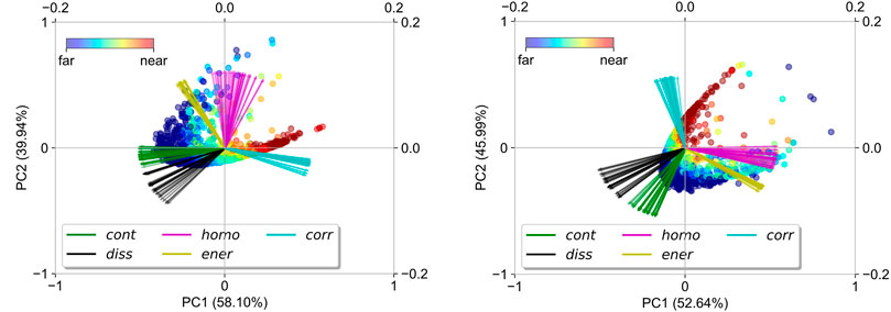
FIGURE 2. Biplots obtained by principal component analysis (PCA) of the standardized GLCM features’ table illustrate variabilities in GLCM features extracted among reference peaks in datasets (A) and (B). The colors of the dots denote their distance from the X-ray photograph of the sediment slide. GLCM features are denoted by arrows in the biplots, and the arrows with the same color denote the same GLCM property derived from different pixel pairs. cont = contrast; homo = homogeneity; corr = correlation; diss = dissimilarity; ener = energy.

The geochemical-context-based peak picking allows us to select peaks that are potentially linked to biogeochemical processes without prior knowledge of their identity, which is of key importance to untargeted data mining. Supplementary Figure S4 shows the ion images of the five most informative peaks (most similar to the X-ray photograph) and the five least informative ones (least similar to the X-ray photograph) in datasets A and B. In dataset A, the two most informative peaks have m/z of 557.252 and 558.255. They likely represent pyropheophorbide a and its ¹³C-isotopologue as Na⁺-adducts, respectively. The C₃₇ di-unsaturated alkenone, which was originally the targeted compound of dataset A in Alfken et al. (2020), is also among the top ranked molecules (fourth, m/z = 553.532) and serves as proof of concept for the ability to detect meaningful compounds with this workflow. In dataset B, the spatial patterns of the five most informative peaks show less laminae-like structure than those in dataset A. The two top ranked molecules can be attributed to chemical formulas C₂₉H₄₈O(Na⁺) and C₂₉H₅₀O(Na⁺) and likely represent sterols, although the specific structures are yet to be determined. Notably, the third–fifth ion images are characterized by the presence of hotspots in addition to the laminae; these hotspots might represent lacustrine debris. In contrast to these most informative molecules, the ion images of the least informative peaks in datasets A and B are rather scattered in the sediment, which agrees with the biplots in Figure 2.

In addition, Supplementary Table S2 shows the rank of some MSI-detectable putatively identified biomarkers after ranking all reference peaks from most informative to least informative. Most of these biomarkers are ranked relatively high. Notably, C₃₇ and C₃₈ alkenones are closely ranked with each other, indicating that they have similar spatial patterns. Interestingly, the two di-unsaturated ones and the two tri-unsaturated ones are, respectively, close to each other, indicating that alkenones with the same unsaturation degree have more similar spatial patterns than those with the same carbon chain length. This agrees with the fact that the degree of unsaturation is susceptible to changing environmental conditions, i.e., SST (Volkman et al., 1980a, Volkman et al., 1980b; Marlowe et al., 1984a, Marlowe et al., 1984b; Brassell et al., 1986). Such consistency demonstrates the power of MSI in revealing the fine spatial patterns of biomarkers in sediments and the capability of geochemical-context-based peak picking in selecting geochemically informative peaks from sedimentary MSI datasets without any prior knowledge of their corresponding molecules. Moreover, the application of geochemical-context-based peak picking is not limited to the MSI datasets obtained from varved SBB sediments as it should also be possible to target geological structures other than sediment laminae.

3.3 Spatial signature identification with NMF

The data cleaning procedures mentioned previously extracted a $18625\times 293$ data matrix (number of spectra $\times$ number of peaks) from dataset A and a $18963\times 323$ data matrix from dataset B, which constitutes an unimaginable information density for a ∼10 cm long sediment section. Repeated NMF was employed to factorize the two resulting matrices in order to extract unique molecular signatures with the associated molecule clusters, in analogy to its most popular use in bioinformatics, i.e., clustering gene expression data and finding the most representative genes of the clusters (Brunet et al., 2004).

3.3.1 Stable spatial signatures and their environmental drivers

The performances of NMF at varying ranks between 3 and 20 are compared in Supplementary Text S2. As a result, an NMF rank of 10 was chosen for both dataset A and dataset B, resulting in the extraction of in total 17 and 14 distinct spatial signatures, respectively, over 30 NMF runs (Supplementary Figures S6, S7). From these, 5 and 10 spatial signatures (Figure 3) are stable because they were reached in at least 27 out of 30 (i.e., >90 percent) NMF runs. The unstable signatures likely represent the local outliers among these stable signatures, but their differences are too trivial to be stably separated. For example, in dataset B, the unstable signature B-NMF12 is in fact similar to the stable signature B-NMF6. Although they are not well-separated from the rank selected in this study, they are in fact separated from each other in the consensus-matrix-based molecular network.

FIGURE 3

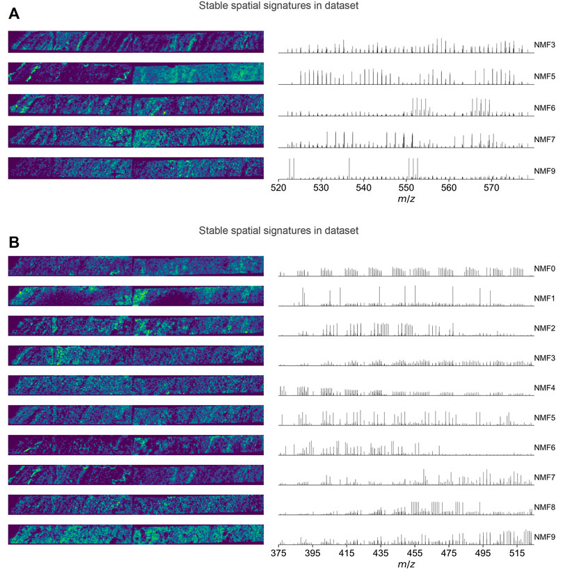
FIGURE 3. Stable spatial signatures discovered in datasets A (A) and B (B). The left figures show the ion images of spatial signatures, i.e., the columns of $W$, the weighted average of all ion images in the cluster, with a color scale in “viridis”, where the lighter colors denote a higher abundance of the signatures. The right figures show the pseudo mass spectrum constructed using the contributions of molecules, i.e., in which peak intensities denote the entries in the rows $H$.

In the following, we compared the spatial signatures with the varved structures of the sediment revealed by its X-ray photograph, and their quarterly averages after applying an age model with the environmental parameters determined in the water column to show that these mathematically derived signatures are indeed relevant to biogeochemical processes. However, one should keep in mind that the inferred ecological and geochemical implications hereafter are speculative and could be oversimplified due to the numerous stereochemical possibilities of the molecular formulas detected, along with other factors. The spatial signatures are coded in the following way: assuming dataset $V\in \{A, B\}$, given $V\sim WH$ for dataset $V$, we refer to the columns in $W$ as signatures and the $k_{th}$ column as a signature $V$-NMFk, whose ion images are denoted by its entries. The contribution of each molecule to a signature $V$-NMFk is denoted by the entries in the $k_{th}$ row of $H$. Although the unstable signatures are worth investigating, for example, B-NMF10 and B-NMF12 show almost complementary ion images (Supplementary Figure S7) that likely indicate distinct sources, only the stable signatures are discussed in the following for succinctly demonstrating the capability of MSI in conjunction with untargeted data mining in extracting biogeochemically relevant molecular signatures from the sediments. For stable signature $V$-NMFk, we show

(1) its ion image that represents the cluster center (the weighted average of all ion images in the cluster; Figure 3, left), constructed using the entries in the $k_{th}$ column of $W$;

(2) the pseudo mass spectrum of each molecule’s contribution (Figure 3, right), i.e., the peak intensities denote the entries in the $k_{th}$ row of $H$;

(3) the associated co-occurrence molecular network constructed using the consensus matrix over multiple NMF runs (Figure 4);

(4) the DTW distance between the quarterly averaged abundance of $V$-NMFk and environmental parameters (Figure 5A), where closer distance suggests a stronger positive correlation, and the DTW distance between the quarterly averaged abundance of $V$-NMFk multiplied by $-1$ (i.e., flipping the temporal sequence upside down) and environmental parameters (Figure 5B), where closer distance suggests stronger negative correlation. Examples of selected best matched signatures and environmental parameters are displayed in Supplementary Figure S8.

FIGURE 4

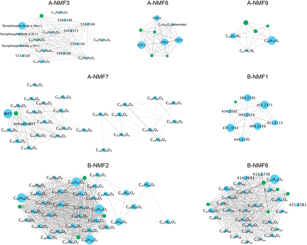
FIGURE 4. Examples of spatially co-occurring molecular networks discovered in datasets (A) and (B). Each node represents a molecule, with the labels being the name of biomarkers, possible chemical formulas, or its m/z ratios. The size of the node denotes the average intensity of the molecule in the dataset. Isotopologues are represented by the green nodes. Edges (lines between the nodes) denote that the two connected nodes are classified into the same cluster for at least 90% of total NMF runs, and thicker edges denote the two connected nodes are clustered together more frequently.

FIGURE 5

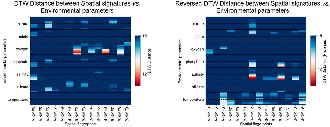
FIGURE 5. (A) DTW distance between the quarterly averaged abundance of the signatures and the environmental parameters integrated over varying depths of water parcel (above the dashed lines: 0—50 m in 10 m increments; below the dashed lines: 50 m—bottom in 100 m increments), where smaller distance indicates stronger positive correlation; (B) DTW distance between the quarterly averaged abundance of the signatures multiplied by $-1$ (i.e., flipping the temporal sequence upside down) and the environmental parameters integrated over varying depths of water parcel (from surface to bottom), where smaller distance indicates stronger negative correlation.

Among all signatures discovered in the two datasets, A-NMF3 shows the most distinct laminations (Figure 3). Figure 6 further shows that the light laminae of A-NMF3 match well with the light diatom ooze laminae of the SBB sediments, which result from enhanced primary production (Schimmelmann and Lange, 1996; Bull et al., 2000). The corresponding molecular network in Figure 4 indicates that A-NMF3 consists of chlorin-like compounds, and the most abundant molecule is putatively pyropheophorbide a. We speculated that pyropheophorbide a and the other chlorin-like compounds in A-NMF3 derive from zooplankton and zoobenthos grazing on diatoms (Head et al., 1994; Szymczak-Żyła et al., 2011), and the distinct light/dark laminae of A-NMF3 may result from the opportunistic bloom-and-bust life cycle of diatoms (Butterfield, 1997). In fact, by comparing the quarterly averaged abundance of A-NMF3 to environmental parameters (Figure 5), we found that the abundance of A-NMF3 is positively correlated with salinity and nutrient concentrations including the concentrations of nitrite, phosphate, and nitrate, while negatively correlated with bottom water oxygen concentrations. The positive correlation could indicate the increase in diatom populations and consequently A-NMF3 associated with increases in nutrient supply (Lange et al., 1997), while the negative correlation could suggest the depletion of oxygen in bottom waters, resulting from the subsequent organic matter remineralization (Reimers et al., 1990; Alfken et al., 2021).

FIGURE 6

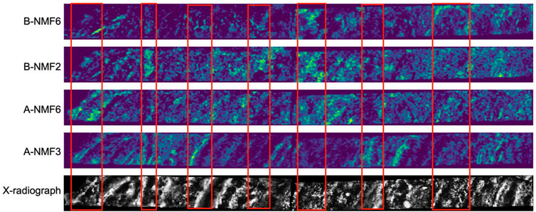
FIGURE 6. Comparison between selected stable spatial signatures and the X-ray photograph of the sediments. The color scale of the ion images is in “viridis”, where the lighter colors denote higher abundance of the signatures.

A-NMF6 consists of alkenones produced by the ubiquitous coccolithophores (Volkman et al., 1980b, 1980a; Marlowe et al., 1984a, Marlowe et al., 1984b), i.e., C₃₇- and C₃₈-, di- and tri-unsaturated alkenones, together with their corresponding isotopologues and a compound with a tentative chemical formula of C₃₇H₇₀O₂, possibly a coccolith derived di-unsaturated alkenoate, e.g., methyl hexatriacontadienoate (Marlowe et al., 1984a; Figure 4). Compared to A-NMF3, A-NMF6 shows less distinct laminations (Figure 6), and its light laminae do not match very well with each other. This agrees with previous observations that coccolithophores usually do not bloom along with diatoms (Zhao et al., 2000). In addition, the quarterly averaged A-NMF6 has a slightly different correlation with environmental parameters compared to A-NMF3 (Figure 5). It is positively correlated with nutrient concentrations, including the concentrations of silicate, phosphate, and nitrate, while negatively correlated with the temperature of the water column. Moreover, although both A-NMF6 and A-NMF3 are negatively correlated with oxygen concentrations in the water column, A-NMF6 is best matched with the oxygen concentrations in the shallower water column, while A-NMF3 is best matched with the oxygen concentrations in the bottom water column.

Although B-NMF6 also shows distinct laminations in its ion image, in contrast to A-NMF3 and A-NMF6, it is more likely to be a terrigenous signal as its light laminae match with the dark laminae of the sediment (Figure 6) formed by seasonal runoff during heavy winter rains (Schimmelmann and Lange, 1996; Bull et al., 2000). MSI also reveals scattered hotspots in B-NMF6 in addition to the laminae couplets, which could indicate the presence of terrigenous particles. The corresponding molecular network of B-NMF2 shows that it consists of steranes and unspecified oxygen-containing compounds (Figure 4). As steranes are not formed from autochthonous organic matter in immature sediments, they are likely derived from eroded source rocks of the Monterey Formation or related oil seeps (Hinrichs et al., 1995); the oxygen-containing compounds with even-numbered carbons, i.e., C₂₄H₄₈O₂, C₂₆H₅₂O₂, and C₂₈H₅₆O₂ could be derived from higher plants (Ratnayake et al., 2005; Kusch et al., 2010). Moreover, the quarterly averaged B-NMF6 is positively correlated with the bottom water oxygen concentrations, while negatively correlated to salinity and nutrient concentrations (Figure 5), which is consistent with its assignment to wintertime terrigenous input during periods of weakened upwelling.

The ion image of B-NMF2 is rather complicated: it is ubiquitous in the sediment, while some of its light laminae (more abundant) match quite well with the dark laminae of the sediment (Figure 6). Hierarchical clustering of the most representative compounds in B-NMF2 displayed in Supplementary Figure S9 further reveals the internal structure of the molecular cluster, which consists of sterols and compounds that have one to three oxygen atoms and double bond equivalents typically found in steroids. Sterols and steroids are known to be produced by diverse species of eukaryotes such as zoo- and phytoplankton and terrestrial plants (Volkman et al., 1998; Volkman, 2003). The mechanism causing the colocalization of these compounds in the sediment deserves further investigation. It is possible that B-NMF2 captures the superimposed signal of steroid-like compounds from varying sources. For example, one of the most abundant molecules in B-NMF2, C₃₀H₅₂O, can be assigned to dinosterol, which is mainly produced by dinoflagellates (Volkman et al., 1993), the algae which often blooms during relaxed upwelling (Kennedy and Brassell, 1992; Smayda and Trainer, 2010). However, the formula is also consistent with terrigenous biomarkers such as lupanol (Pancost et al., 2002) or the bacterial biomarker hopanol (Pearson et al., 2001). Alternatively, B-NMF2 could reflect benthic biogeochemical processes because of its strong positive correlation to bottom water oxygen concentration and strong negative correlation to bottom water salinity and phosphate concentrations (Figure 5).

The other signatures exhibit distinctive spatial patterns as well, although not all chemical formulas of the associated molecules can be assigned with certainty, partly due to the absence of isotopologue peaks. For example, signatures A-NMF5 and B-NMF7 are both characterized by the “intrusion” structure in the uppermost ∼5 cm sediment in addition to the dark and light laminae (Figure 3); such a structure is also visible on the sediment slide. A-NMF7 is omnipresent in the sediment, with distinct laminations only visible in the topmost sediment, and it consists of a large number of molecules, with the most abundant one likely to be bacteriohopanetetrol (Figure 4). Quarterly averaged A-NMF7 is positively correlated with silicate concentration but negatively correlated with temperature and nitrite concentration (Figure 5). A-NMF9 is of low abundance in the topmost surface sediment, and it is associated with three compounds that are apparently homologs, together with their ¹³C isotopologues. Notably, A-NMF9 does not show a strong correlation with any environmental parameters. In addition, B-NMF1 is characterized by curved dark/light boundaries in the sediment (Figure 3). We speculated that they are polyethylene glycol contaminants (PEG; H⁺ and Na⁺ adducts) because of the characteristic mass difference of 44 Da between individual molecules (Figure 4). Moreover, it should be noted that all the signatures discovered in this study spatially overlap with each other to some extent, causing image segmentation to be difficult. This is due to either a blurred zonation of biomarkers or the relatively small mass window analyzed, which limits the number of diagnostic biomarkers.

3.3.2 Potential of supervised learning for novel molecular proxy discovery

The proposed data processing workflow in this study is explorative and mostly unsupervised as except in the geochemical-context-based peak picking step, it only utilizes the information carried by sedimentary MSI datasets themselves. In order to demonstrate the potential of supervised learning approaches for novel molecular proxy discovery on the basis of data mining results, we trained linear models for indicating SST and sediment-water interface redox conditions, using the abundances of co-occurring molecules associated with clusters A-NMF6 (alkenones and derivatives) and B-NMF2 (incl. steroid-like compounds), respectively, based on the assumption that residuals among these co-occurring molecules are not random and result from biogeochemical influences such as changing environmental conditions or selectivity in biogeochemical processes. ElasticNet, a popular regularized linear regression algorithm implemented in the python package scikit-learn (Pedregosa et al., 2011), was employed to tackle multicollinearity (Gunst and Webster, 1975; Alin, 2010). Time-based cross-validation implemented in scikit-learn (Pedregosa et al., 2011) was employed to reduce overfitting and autocorrelation; whether the derived proxies are applicable in longer time series or at other sites is beyond the scope of this study.

Since it has been established that in dataset A, the $U_{37}^{K^{\prime }}$ index has a strong correlation with SST (Alfken et al., 2020), we first validated the use of ElasticNet on the alkenone cluster A-NMF6 and its relationship to SST. Although A-NMF6 contains four ¹³C isotopologues and an alkenoate in addition to the monoisotopic alkenones, the whole cluster is used for training without removing any peaks in order to show the reliability of ElasticNet with redundant variables. Figure 7A compares the SST measured in the water column and the SST indicated by the trained model and the $U_{37}^{K^{\prime }}$ index, suggesting that the model trained in this study indicates changes in SST. Supplementary Table 3 shows the resulting coefficients assigned to the nine molecules in A-NMF6 after cross-validated ElasticNet training and indicates that the two di-unsaturated alkenones and their isotopologues are positively correlated with SST, while the two tri-unsaturated alkenones and their isotopologues are negatively correlated with SST. This is in agreement with the definition of the $U_{37}^{K^{\prime }}$ index proposed in the previous study (Prahl and Wakeham, 1987). In addition, the putative alkenoate was assigned with a negative coefficient after training, although it weighed less than the two tri-unsaturated alkenones. This may suggest that the molecule is also regulated by coccolithophores to adapt to changing SST, which agrees with the observation by Conte et al. (1998) that the cellular ratio of alkenoates to alkenones in coccolithophores decreases with increasing water temperature.

FIGURE 7

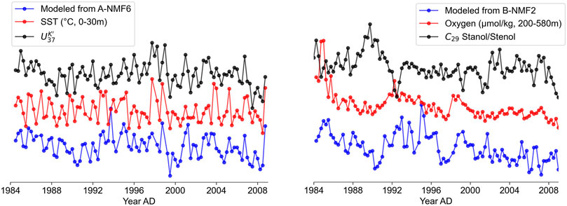
FIGURE 7. (A) Comparison between the ElasticNet model trained by A-NMF6, SST, and $U_{37}^{K^{\prime }}$ ratio (Alfken et al., 2020); (B) comparison between the ElasticNet model trained by B-NMF2, bottom water oxygen concentrations, and the C₂₉ stanol/stenol ratio (Alfken et al., 2021). In both figures, the vertical axes of the time series are staggered (i.e., adjusted along the vertical axes to avoid overlap) for better visualization.

B-NMF2 consists of diverse steroid-like compounds with one or more oxygen-containing functional groups, which might be sensitive to redox conditions. We further applied ElasticNet to train a model for indicating bottom water redox conditions using the abundances of co-localized molecules in B-NMF2 against bottom water oxygen concentrations. Figure 7B compares the bottom water oxygen concentrations with the trained model and the redox-sensitive C₂₉ stanol/stenol ratio. In contrast to the model for indicating SST (cf. in Supplementary Table S3), the resulting coefficients for indicating redox conditions are all equal or greater than 0, with smaller absolute values (Supplementary Table S4). The non-negative coefficients of the compounds suggest that variations in the model could be driven by 1) the relative abundances amongst these steroid-like compounds in B-NMF2 or 2) the relative abundance of these steroid-like compounds as a group compared to all other compounds in the spectrum. Although all non-negative coefficients could make the model less favorable as a paleoenvironmental proxy and more sophisticated nonlinear models are likely required to characterize the link between these compounds and the redox condition, such rather complicated supervised learning approaches are beyond the scope of this study and will be evaluated in our future work. Since standard scaling was applied before model training, the magnitudes of resulting coefficients depend largely on the number of dependent variables. The smaller absolute coefficients assigned in B-NMF2 compared to those assigned in A-NMF6 results from the much larger numbers of variables (molecules) in B-NMF2. Nevertheless, the resulting coefficients agree with the observation in the aforementioned section that B-NMF2 is positively correlated with bottom water oxygen concentrations, and the ElasticNet model, here, further extracted the most redox-related biomarkers from B-NMF2. It is interesting that the top three molecules are all C₃₀ pentacyclic triterpenoids with varying unsaturation degrees. This may suggest that they are the most recalcitrant components of B-NMF2 in the sediment. However, other factors cannot be ruled out, for example, it is also possible that the three putative C₃₀ pentacyclic triterpenoids have the strongest contribution from terrestrial input during the winter season as compounds with the same chemical formulas have been reported in higher plants (e.g., Escobedo et al., 2012; Kennedy, 2012).

4 Conclusion

This study introduced an untargeted data processing workflow, including data cleaning and untargeted data mining, for sedimentary MSI datasets and evaluated the workflow by re-analyzing two existing MSI datasets obtained from ∼10 cm SBB sediment sections. Bin-wise KDE employed for peak detection and alignment extracted more than a thousand peaks from each dataset and achieved an average mass deviation of 0.84 ppm between the resulting reference m/z and the theoretical m/z of 18 established biomarkers detected by MSI in this study. The detected peaks were then evaluated by the peak-prominence filter that measures the sparsity of these peaks in sediments, in conjunction with the geochemical-context-based filter that measures the distance of the ion images of these peaks from the X-ray photograph of the sediment, allowing the selection of hundreds of biogeochemically informative peaks that exhibit spatial patterns reminiscent of the sediment laminae. The subsequent untargeted data mining using repeated NMF further extracted a total of 15 stable molecular signatures from these hundreds of informative peaks. The relevance between these mathematically derived signatures and historical oceanographic data proves the capability of the proposed workflow in extracting biogeochemically relevant molecular signatures from the sedimentary MSI datasets, broadening the number and diversity of available candidate compounds utilizable for molecular stratigraphy. On the basis of these molecular signatures, ElasticNet, a supervised learning algorithm, combined with cross-validation was able to train easy-to-interpret multivariate linear regression models using the residuals among co-occurring molecules against historical oceanographic data for paleoenvironmental and paleoceanographic reconstruction, and it holds great potential for novel biomarker discovery in a top-down manner and unleashing the full power of MSI in the field of organic geochemistry.

Data availability statement

The datasets presented in this study can be found in online repositories. The names of the repository/repositories and accession number(s) can be found at: https://www.ebi.ac.uk/metabolights/MTBLS4609.

Author contributions

WL, SA, LW, JL, and KH contributed to the conception and design of the study. SA collected the samples and performed the experiment. WL compiled the data processing workflow and wrote the corresponding codes. WL wrote the first draft of the manuscript. All authors contributed to manuscript revision, read, and approved the submitted version.

Acknowledgments

This research was funded by the European Research Council under the European Union’s Horizon 2020 Research and Innovation Programme (grant agreement No. 670115 ZOOMECULAR; PI Kai-Uwe Hinrichs). Additional support has been provided by Germany’s Excellence Strategy—EXC-2077—390741603. The authors also thank the developers of Python, scikit-learn, scipy, and all other open-source libraries employed in the data processing workflow in this study.

Conflict of interest

The authors declare that the research was conducted in the absence of any commercial or financial relationships that could be construed as a potential conflict of interest.

Publisher’s note

All claims expressed in this article are solely those of the authors and do not necessarily represent those of their affiliated organizations, or those of the publisher, the editors, and the reviewers. Any product that may be evaluated in this article, or claim that may be made by its manufacturer, is not guaranteed or endorsed by the publisher.

Supplementary material

The Supplementary Material for this article can be found online at: https://www.frontiersin.org/articles/10.3389/feart.2022.931157/full#supplementary-material

References

Alexandrov, T. (2012). MALDI imaging mass spectrometry: Statistical data analysis and current computational challenges. BMC Bioinforma. 13, S11. doi:10.1186/1471-2105-13-S16-S11

PubMed Abstract | CrossRef Full Text | Google Scholar

Alexandrov, T. (2020). Spatial metabolomics and imaging mass spectrometry in the age of artificial intelligence. Annu. Rev. Biomed. Data Sci. 3, 61–87. doi:10.1146/annurev-biodatasci-011420-031537

PubMed Abstract | CrossRef Full Text | Google Scholar

Alfken, S., Wörmer, L., Lipp, J. S., Napier, T., Elvert, M., Wendt, J., et al. (2021). Disrupted coherence between upwelling strength and redox conditions reflects source water change in Santa Barbara Basin during the 20th century. Paleoceanogr. Paleoclimatol. 36, e2021PA004354. doi:10.1029/2021PA004354

CrossRef Full Text | Google Scholar

Alfken, S., Wörmer, L., Lipp, J. S., Wendt, J., Schimmelmann, A., Hinrichs, K.-U., et al. (2020). Mechanistic insights into molecular proxies through comparison of subannually resolved sedimentary records with instrumental water column data in the Santa Barbara Basin, Southern California. Paleoceanogr. Paleoclimatol. 35, e2020PA004076. doi:10.1029/2020PA004076

CrossRef Full Text | Google Scholar

Alfken, S., Wörmer, L., Lipp, J. S., Wendt, J., Taubner, H., Schimmelmann, A., et al. (2019). Micrometer scale imaging of sedimentary climate archives – sample preparation for combined elemental and lipid biomarker analysis. Org. Geochem. 127, 81–91. doi:10.1016/j.orggeochem.2018.11.002

CrossRef Full Text | Google Scholar

Alin, A. (2010). Multicollinearity. WIREs Comput. Stat. 2, 370–374. doi:10.1002/wics.84

CrossRef Full Text | Google Scholar

Botev, Z. I., Grotowski, J. F., and Kroese, D. P. (2010). Kernel density estimation via diffusion. Ann. Stat. 38. doi:10.1214/10-AOS799

CrossRef Full Text | Google Scholar

Brassell, S. C., Eglinton, G., Marlowe, I. T., Pflaumann, U., and Sarnthein, M. (1986). Molecular stratigraphy: A new tool for climatic assessment. Nature 320, 129–133. doi:10.1038/320129a0

CrossRef Full Text | Google Scholar

Brunet, J.-P., Tamayo, P., Golub, T. R., and Mesirov, J. P. (2004). Metagenes and molecular pattern discovery using matrix factorization. Proc. Natl. Acad. Sci. U. S. A. 101, 4164–4169. doi:10.1073/pnas.0308531101

PubMed Abstract | CrossRef Full Text | Google Scholar

Bull, D., Kemp, A. E. S., and Weedon, G. P. (2000). A 160-k.y.-old record of el niño–southern oscillation in marine production and coastal runoff from Santa Barbara Basin, California, USA. Geol. 28, 1007. doi:10.1130/0091-7613(2000)28<1007:akroen>2.0.co;2

CrossRef Full Text | Google Scholar

Butterfield, N. J. (1997). Plankton ecology and the Proterozoic-phanerozoic transition. Paleobiology 23, 247–262. doi:10.1017/S009483730001681X

CrossRef Full Text | Google Scholar

CalCOFI (2018). California cooperative oceanic Fisheries investigation (CalCOFI), march 2018. AvaliableAt: http://www.calcofi.org.

Google Scholar

Comon, P. (1994). Independent component analysis, a new concept? Signal Process. 36, 287–314. doi:10.1016/0165-1684(94)90029-9

CrossRef Full Text | Google Scholar

Conte, M. H., Thompson, A., Lesley, D., and Harris, R. P. (1998). Genetic and physiological influences on the alkenone/alkenoate versus growth temperature relationship in Emiliania Huxleyi and Gephyrocapsa Oceanica. Geochim. Cosmochim. Acta 62, 51–68. doi:10.1016/S0016-7037(97)00327-X

CrossRef Full Text | Google Scholar

Damsté, J. S. S., Kohnen, M. E. L., and de Leeuw, J. W. (1990). Thiophenic biomarkers for palaeoenvironmental assessment and molecular stratigraphy. Nature 345, 609–611. doi:10.1038/345609a0

CrossRef Full Text | Google Scholar

Deininger, S.-O., Cornett, D. S., Paape, R., Becker, M., Pineau, C., Rauser, S., et al. (2011). Normalization in MALDI-TOF imaging datasets of proteins: Practical considerations. Anal. Bioanal. Chem. 401, 167–181. doi:10.1007/s00216-011-4929-z

PubMed Abstract | CrossRef Full Text | Google Scholar

Eriksson, J. O., Rezeli, M., Hefner, M., Marko-Varga, G., and Horvatovich, P. (2019). Clusterwise peak detection and filtering based on spatial distribution to efficiently mine mass spectrometry imaging data. Anal. Chem. 91, 11888–11896. doi:10.1021/acs.analchem.9b02637

PubMed Abstract | CrossRef Full Text | Google Scholar

Escobedo, C., Lozada, M., Hernández-Ortega, S., Villarreal, M., Gnecco, D., Enriquez, R., et al. (2012). 108. ¹H and ¹³C NMR characterization of new cycloartane triterpenes from Mangifera indica. Magn. Reson. Chem. 50, 52–57. doi:10.1002/mrc.2836

PubMed Abstract | CrossRef Full Text | Google Scholar

Eyssen, H. J., Parmentier, G. G., Compernolle, F. C., de Pauw, G., and Piessens-Denef, M. (1973). Biohydrogenation of sterols by eubacterium ATCC 21, 408—nova species. Eur. J. Biochem. 36, 411–421. doi:10.1111/j.1432-1033.1973.tb02926.x

PubMed Abstract | CrossRef Full Text | Google Scholar

Fonville, J. M., Carter, C., Cloarec, O., Nicholson, J. K., Lindon, J. C., Bunch, J., et al. (2012). Robust data processing and normalization strategy for MALDI mass spectrometric imaging. Anal. Chem. 84, 1310–1319. doi:10.1021/ac201767g

PubMed Abstract | CrossRef Full Text | Google Scholar

Gut, Y., Boiret, M., Bultel, L., Renaud, T., Chetouani, A., Hafiane, A., et al. (2015). Application of chemometric algorithms to MALDI mass spectrometry imaging of pharmaceutical tablets. J. Pharm. Biomed. 105, 91–100.

PubMed Abstract | CrossRef Full Text | Google Scholar

Gunst, R. F., and Webster, J. T. (1975). Regression analysis and problems of multicollinearity. Commun. Stat. Simul. Comput. 4, 277–292. doi:10.1080/03610927308827246

CrossRef Full Text | Google Scholar

Hall-Beyer, M. (2017). GLCM texture: A tutorial v.3.0 march 2017. AvaliableAt: http://www.ucalgary.ca/UofC/nasdev/mhallbey/research.htm.

Google Scholar

Haralick, R. M., Shanmugam, K., and Dinstein, I. (1973). Textural features for image classification. IEEE Trans. Syst. Man. Cybern. 3, 610–621. doi:10.1109/TSMC.1973.4309314

CrossRef Full Text | Google Scholar

Haug, K., Cochrane, K., Nainala, V. C., Williams, M., Chang, J., Jayaseelan, K. V., et al. (2020). MetaboLights: A resource evolving in response to the needs of its scientific community. Nucleic Acids Res. 48 (D1), D440–D444.

PubMed Abstract | CrossRef Full Text | Google Scholar

Hayes, J. M., Freeman, K. H., Popp, B. N., and Hoham, C. H. (1990). Compound-specific isotopic analyses: A novel tool for reconstruction of ancient biogeochemical processes. Org. Geochem. 16, 1115–1128. doi:10.1016/0146-6380(90)90147-R

PubMed Abstract | CrossRef Full Text | Google Scholar

Head, E. J. H., Hargrave, B. T., and Subba Rao, D. V. (1994). Accumulation of a pheophorbide a-like pigment in sediment traps during late stages of a spring bloom: A product of dying algae? Limnol. Oceanogr. 39, 176–181. doi:10.4319/lo.1994.39.1.0176

CrossRef Full Text | Google Scholar

Hinrichs, K.-U., Rullkötter, J., and Stein, R. (1995). Preliminary assessment of organic geochemical signals in sediments from hole 893A, Santa Barbara Basin, offshore California. Proc. Odp. Sci. Results 146, 201–211.

CrossRef Full Text | Google Scholar

Hinrichs, K.-U., Schneider, R. R., Müller, P. J., and Rullkötter, J. (1999). A biomarker perspective on paleoproductivity variations in two Late Quaternary sediment sections from the Southeast Atlantic Ocean. Org. Geochem. 30, 341–366. doi:10.1016/S0146-6380(99)00007-8

CrossRef Full Text | Google Scholar

Huang, Y., Street-Perrott, F. A., Perrott, R. A., Metzger, P., and Eglinton, G. (1999). Glacial–interglacial environmental changes inferred from molecular and compound-specific δ¹³C analyses of sediments from Sacred Lake, Mt. Kenya. Geochim. Cosmochim. Acta 63, 1383–1404. doi:10.1016/S0016-7037(99)00074-5

CrossRef Full Text | Google Scholar

Hülsemann, J., and Emery, K. O. (1961). Stratification in recent sediments of Santa Barbara Basin as controlled by organisms and water character. J. Geol. 69, 279–290. doi:10.1086/626742

CrossRef Full Text | Google Scholar

Jolliffe I. T. (Editor) (2002). “Principal component analysis for special types of data,” Principal component analysis springer series in statistics (New York, NY: Springer), 338–372. doi:10.1007/0-387-22440-8_13

CrossRef Full Text | Google Scholar

Jutten, C., and Herault, J. (1991). Blind separation of sources, part I: An adaptive algorithm based on neuromimetic architecture. Signal Process. 24, 1–10. doi:10.1016/0165-1684(91)90079-X

CrossRef Full Text | Google Scholar

Kennedy, J. A., and Brassell, S. C. (1992). Molecular stratigraphy of the Santa Barbara Basin: Comparison with historical records of annual climate change. Org. Geochem. 19, 235–244. doi:10.1016/0146-6380(92)90040-5

CrossRef Full Text | Google Scholar

Kennedy, M. L. (2012). Phytochemical profile of the stems of Aeonium lindleyi. Rev. Bras. Farmacogn. 22, 676–679. doi:10.1590/S0102-695X2012005000037

CrossRef Full Text | Google Scholar

Kim, H., and Park, H. (2007). Sparse non-negative matrix factorizations via alternating non-negativity-constrained least squares for microarray data analysis. Bioinformatics 23, 1495–1502. doi:10.1093/bioinformatics/btm134

PubMed Abstract | CrossRef Full Text | Google Scholar

Kusch, S., Rethemeyer, J., Schefuß, E., and Mollenhauer, G. (2010). Controls on the age of vascular plant biomarkers in Black Sea sediments. Geochim. Cosmochim. Acta 74, 7031–7047. doi:10.1016/j.gca.2010.09.005

CrossRef Full Text | Google Scholar

Lange, C., Weinheimer, A., Reid, F., and Thunell, R. (1997). Sedimentation patterns of diatoms, radiolarians, and silicoflagellates in Santa Barbara Basin, California. Calif. Coop. Ocean. Fish. Investig. Rep. 38, 161–170.

Google Scholar

Marlowe, I. T., Brassell, S. C., Eglinton, G., and Green, J. C. (1984a). Long chain unsaturated ketones and esters in living algae and marine sediments. Org. Geochem. 6, 135–141. doi:10.1016/0146-6380(84)90034-2

CrossRef Full Text | Google Scholar

Marlowe, I. T., Green, J. C., Neal, A. C., Brassell, S. C., Eglinton, G., Course, P. A., et al. (1984b). Long chain (nC₃₇–C₃₉) alkenones in the Prymnesiophyceae. Distribution of alkenones and other lipids and their taxonomic significance. Br. Phycol. J. 19, 203–216. doi:10.1080/00071618400650221

CrossRef Full Text | Google Scholar

Mittal, P., Condina, M. R., Klingler-Hoffmann, M., Kaur, G., Oehler, M. K., Sieber, O. M., et al. (2021). Cancer tissue classification using supervised machine learning applied to MALDI mass spectrometry imaging. Cancers 13, 5388. doi:10.3390/cancers13215388

PubMed Abstract | CrossRef Full Text | Google Scholar

Nijs, M., Smets, T., Waelkens, E., and De Moor, B. (2021). A mathematical comparison of non-negative matrix factorization related methods with practical implications for the analysis of mass spectrometry imaging data. Rapid Commun. Mass Spectrom. 35 (21), e9181.

PubMed Abstract | CrossRef Full Text | Google Scholar

Nishimura, M., and Koyama, T. (1977). The occurrence of stanols in various living organisms and the behavior of sterols in contemporary sediments. Geochim. Cosmochim. Acta 41, 379–385. doi:10.1016/0016-7037(77)90265-4

CrossRef Full Text | Google Scholar

Odland, T. (2018). tommyod/KDEpy: Kernel density estimation in Python. Zenodo. doi:10.5281/zenodo.2392268

CrossRef Full Text | Google Scholar

Ovchinnikova, K., Stuart, L., Rakhlin, A., Nikolenko, S., and Alexandrov, T. (2020). ColocML: Machine learning quantifies co-localization between mass spectrometry images. Bioinformatics 36, 3215–3224. doi:10.1093/bioinformatics/btaa085

PubMed Abstract | CrossRef Full Text | Google Scholar

Pancost, R. D., Baas, M., van Geel, B., and Sinninghe Damsté, J. S. (2002). Biomarkers as proxies for plant inputs to peats: An example from a sub-boreal ombrotrophic bog. Org. Geochem. 33, 675–690. doi:10.1016/S0146-6380(02)00048-7

CrossRef Full Text | Google Scholar

Pearson, A., McNichol, A. P., Benitez-Nelson, B. C., Hayes, J. M., and Eglinton, T. I. (2001). Origins of lipid biomarkers in Santa monica basin surface sediment: A case study using compound-specific Δ¹⁴C analysis. Geochim. Cosmochim. Acta 65, 3123–3137. doi:10.1016/S0016-7037(01)00657-3

CrossRef Full Text | Google Scholar

Pedregosa, F., Varoquaux, G., Gramfort, A., Michel, V., Thirion, B., Grisel, O., et al. (2011). Scikit-learn: Machine learning in Python. J. Mach. Learn. Res. 12, 2825–2830.

Google Scholar

Peters, K. E., Peters, K. E., Walters, C. C., and Moldowan, J. M. (2005). The biomarker guide. Cambridge, United Kingdom: Cambridge University Press.

Google Scholar

Prahl, F. G., and Wakeham, S. G. (1987). Calibration of unsaturation patterns in long-chain ketone compositions for palaeotemperature assessment. Nature 330, 367–369. doi:10.1038/330367a0

CrossRef Full Text | Google Scholar

Quanico, J., Franck, J., Wisztorski, M., Salzet, M., and Fournier, I. (2017). “Progress and potential of imaging mass spectrometry applied to biomarker discovery,” in Neuroproteomics: Methods and protocols methods in molecular biology. Editors F. H. Kobeissy, and M. Stevens Stanley (New York, NY: Springer), 21–43. doi:10.1007/978-1-4939-6952-4_2

CrossRef Full Text | Google Scholar

Ratnayake, N. P., Suzuki, N., and Matsubara, M. (2005). Sources of long chain fatty acids in deep sea sediments from the Bering Sea and the North Pacific Ocean. Org. Geochem. 36, 531–541. doi:10.1016/j.orggeochem.2004.11.004

CrossRef Full Text | Google Scholar

Reimers, C. E., Lange, C. B., Tabak, M., and Bernhard, J. M. (1990). Seasonal spillover and varve formation in the Santa Barbara Basin, California. Limnol. Oceanogr. 35, 1577–1585. doi:10.4319/lo.1990.35.7.1577

CrossRef Full Text | Google Scholar

Rosenfeld, R. S., and Hellman, L. (1971). Reduction and esterification of cholesterol and sitosterol by homogenates of feces. J. Lipid Res. 12, 192–197. doi:10.1016/S0022-2275(20)39529-8

PubMed Abstract | CrossRef Full Text | Google Scholar

Schimmelmann, A., and Lange, C. B. (1996). Tales of 1001 varves: A review of Santa Barbara Basin sediment studies. Geol. Soc. Lond. Spec. Publ. 116, 121–141. doi:10.1144/GSL.SP.1996.116.01.12

CrossRef Full Text | Google Scholar

Siy, P. W., Moffitt, R. A., Parry, R. M., Chen, Y., Liu, Y., Sullards, M. C., et al. (2008). “Matrix factorization techniques for analysis of imaging mass spectrometry data,” in 8th IEEE International Conference on BioInformatics and BioEngineering, 1–6.

CrossRef Full Text | Google Scholar

Smayda, T. J., and Trainer, V. L. (2010). Dinoflagellate blooms in upwelling systems: Seeding, variability, and contrasts with diatom bloom behaviour. Prog. Oceanogr. 85, 92–107. doi:10.1016/j.pocean.2010.02.006

CrossRef Full Text | Google Scholar

Soutar, A., and Crill, P. A. (1977). Sedimentation and climatic patterns in the Santa Barbara Basin during the 19th and 20th centuries. GSA Bull. 88, 1161–1172. doi:10.1130/0016-7606(1977)88<1161:SACPIT>2.0.CO;2

CrossRef Full Text | Google Scholar

Summons, R. E., Welander, P. V., and Gold, D. A. (2022). Lipid biomarkers: Molecular tools for illuminating the history of microbial life. Nat. Rev. Microbiol. 20, 174–185. doi:10.1038/s41579-021-00636-2

PubMed Abstract | CrossRef Full Text | Google Scholar

Szymczak-Żyła, M., Kowalewska, G., and Louda, J. W. (2011). Chlorophyll-a and derivatives in recent sediments as indicators of productivity and depositional conditions. Mar. Chem. 125, 39–48. doi:10.1016/j.marchem.2011.02.002

CrossRef Full Text | Google Scholar

Thiele, H., Heldmann, S., Trede, D., Strehlow, J., Wirtz, S., Dreher, W., et al. (2014). 2D and 3D MALDI-imaging: Conceptual strategies for visualization and data mining. Biochimica Biophysica Acta - Proteins Proteomics 1844, 117–137. doi:10.1016/j.bbapap.2013.01.040

PubMed Abstract | CrossRef Full Text | Google Scholar

Thunell, R. C., Tappa, E., and Anderson, D. M. (1995). Sediment fluxes and varve formation in Santa Barbara Basin, offshore California. Geol. 23, 1083. doi:10.1130/0091-7613(1995)023<1083:SFAVFI>2.3.CO;2

CrossRef Full Text | Google Scholar

Trede, D., Kobarg, J. H., Oetjen, J., Thiele, H., Maass, P., Alexandrov, T., et al. (2012). On the importance of mathematical methods for analysis of MALDI-imaging mass spectrometry data. J. Integr. Bioinform. 9, 1–11. doi:10.1515/jib-2012-189

PubMed Abstract | CrossRef Full Text | Google Scholar

van der Walt, S., Schönberger, J. L., Nunez-Iglesias, J., Boulogne, F., Warner, J. D., Yager, N., et al. (2014). Scikit-image: Image processing in Python. PeerJ 2, e453. doi:10.7717/peerj.453

PubMed Abstract | CrossRef Full Text | Google Scholar

Verbeeck, N., Caprioli, R. M., and Van de Plas, R. (2020). Unsupervised machine learning for exploratory data analysis in imaging mass spectrometry. Mass Spectrom. Rev. 39, 245–291. doi:10.1002/mas.21602

PubMed Abstract | CrossRef Full Text | Google Scholar

Virtanen, P., Gommers, R., Oliphant, T. E., Haberland, M., Reddy, T., Cournapeau, D., et al. (2020). SciPy 1.0: Fundamental algorithms for scientific computing in Python. Nat. Methods 17, 261–272. doi:10.1038/s41592-019-0686-2

PubMed Abstract | CrossRef Full Text | Google Scholar

Volkman, J. K., Barrett, S. M., Blackburn, S. I., Mansour, M. P., Sikes, E. L., Gelin, F., et al. (1998). Microalgal biomarkers: A review of recent research developments. Org. Geochem. 29, 1163–1179. doi:10.1016/S0146-6380(98)00062-X

CrossRef Full Text | Google Scholar

Volkman, J. K., Barrett, S. M., Dunstan, G. A., and Jeffrey, S. W. (1993). Geochemical significance of the occurrence of dinosterol and other 4-methyl sterols in a marine diatom. Org. Geochem. 20, 7–15. doi:10.1016/0146-6380(93)90076-N

CrossRef Full Text | Google Scholar

Volkman, J. K., Eglinton, G., Corner, E. D. S., and Forsberg, T. E. V. (1980a). Long-chain alkenes and alkenones in the marine coccolithophorid Emiliania huxleyi. Phytochemistry 19, 2619–2622. doi:10.1016/S0031-9422(00)83930-8

CrossRef Full Text | Google Scholar

Volkman, J. K., Eglinton, G., Corner, E. D. S., and Sargent, J. R. (1980b). Novel unsaturated straight-chain C₃₇–C₃₉ methyl and ethyl ketones in marine sediments and a coccolithophore Emiliania huxleyi. Phys. Chem. Earth. 12, 219–227. doi:10.1016/0079-1946(79)90106-X

CrossRef Full Text | Google Scholar

Volkman, J. (2003). Sterols in microorganisms. Appl. Microbiol. Biotechnol. 60, 495–506. doi:10.1007/s00253-002-1172-8

PubMed Abstract | CrossRef Full Text | Google Scholar

Wakeham, S. G. (1989). Reduction of stenols to stanols in particulate matter at oxic–anoxic boundaries in sea water. Nature 342, 787–790. doi:10.1038/342787a0

CrossRef Full Text | Google Scholar

Wannesm, K., Yurtman, A., Robberechts, P., Vohl, D., and Ma, E. (2022). wannesm/dtaidistance: v2.3.5. Zenodo. doi:10.5281/ZENODO.5901139

CrossRef Full Text | Google Scholar

Wijetunge, C. D., Saeed, I., Boughton, B. A., Spraggins, J. M., Caprioli, R. M., Bacic, A., et al. (2015). Exims: An improved data analysis pipeline based on a new peak picking method for EXploring Imaging Mass Spectrometry data. Bioinformatics 31, 3198–3206. doi:10.1093/bioinformatics/btv356

PubMed Abstract | CrossRef Full Text | Google Scholar

Wörmer, L., Elvert, M., Fuchser, J., Lipp, J. S., Buttigieg, P. L., Zabel, M., et al. (2014). Ultra-high-resolution paleoenvironmental records via direct laser-based analysis of lipid biomarkers in sediment core samples. Proc. Natl. Acad. Sci. U. S. A. 111, 15669–15674. doi:10.1073/pnas.1405237111

PubMed Abstract | CrossRef Full Text | Google Scholar

Wörmer, L., Gajendra, N., Schubotz, F., Matys, E. D., Evans, T. W., Summons, R. E., et al. (2020). A micrometer-scale snapshot on phototroph spatial distributions: Mass spectrometry imaging of microbial mats in Octopus spring, yellowstone national Park. Geobiology 18, 742–759. doi:10.1111/gbi.12411

PubMed Abstract | CrossRef Full Text | Google Scholar

Wörmer, L., Wendt, J., Alfken, S., Wang, J.-X., Elvert, M., Heuer, V. B., et al. (2019). Towards multiproxy, ultra-high resolution molecular stratigraphy: Enabling laser-induced mass spectrometry imaging of diverse molecular biomarkers in sediments. Org. Geochem. 127, 136–145. doi:10.1016/j.orggeochem.2018.11.009

CrossRef Full Text | Google Scholar

Zhang, Y., Wen, Z., Washburn, M. P., and Florens, L. (2011). Improving proteomics mass accuracy by dynamic offline lock mass. Anal. Chem. 83, 9344–9351. doi:10.1021/ac201867h

PubMed Abstract | CrossRef Full Text | Google Scholar

Zhao, M., Eglinton, G., Read, G., and Schimmelmann, A. (2000). An alkenone () quasi-annual sea surface temperature record (A.D. 1440 to 1940) using varved sediments from the Santa Barbara Basin. Org. Geochem. 31, 903–917. doi:10.1016/S0146-6380(00)00034-6

CrossRef Full Text | Google Scholar