Atmospheric conditions conducive to marine fog over the northeast Pacific in winters of 1979–2019

1 Introduction

Marine fog occurs over oceans and coastal regions when tiny water droplets sustain in the atmospheric boundary layer and cause the degradation of atmospheric horizontal visibility to less than 1 km (Wang, 1985). The low visibility in marine fog may cause ship damages, casualties, and economic losses (Gultepe et al., 2007).

The midlatitude region of the northwest Pacific (NWP) is the foggiest area worldwide. The annual marine fog frequency (MFF) is up to 23% (Fu and Song, 2014) and reaches 59.8% in summer (June–August) (Dorman et al., 2017). The large-scale circulation associated with marine fog in the NWP has been analyzed in previous literature. Sugimoto et al. (2013) indicate that the strengthened Okhotsk high and suppression of the northward extension of the northern Pacific surface high (NPSH) were responsible for the declining trend of MFF during 1931–2010 at Kushiro, Hokkaido, in July. Zhang et al. (2015) suggest that the position and orientation of the NPSH is the most important factor influencing the MFF in the NWP.

In a cold season (November–February), fog rarely occurs over the NWP, and the MFF is close to zero, under the influence of the cold winter monsoon from the Asian continent (Wang, 1985). However, the MFF over the northeast Pacific (NEP) is higher than the MFF over the NWP, with a maximum of 11% (Figure 1). It is unclear why marine fog often occurs in winter in the NEP. Some of the differences are because of specifics of atmospheric forcing that generates a separation of the North Pacific (NP) in winter into the eastern and western parts. By using the EOF computation of NCEP/NCAR reanalysis data (Kalnay et al., 1996) for 1948–2011, Xia et al. (2016) showed distinct synoptic-scale eddy regions at 850 hPa in winter in the eastern and western Pacific.

FIGURE 1

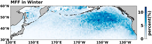
FIGURE 1. Spatial distribution of MFF (%) over the north Pacific in winter (derived from the ICOADS observations).

NEP should be also viewed in the context of long-term variability of main parameters. Based on an analysis of century-long observations, Johnstone and Mantua (2014) show that there is a warming trend over the NEP in the coastal sea surface temperature (SST) and sensible heat flux, while their negative trends are over the north-central Pacific (NCP). They attributed the warming trends to changes in atmospheric conditions and low interdecadal variability in surface-level pressure anomalies. This should also bear importance on understanding the climatology of marine fog, its frequency, and possible trends.

Previous studies indicate that marine fog can form over the cold sea surface under the conditions of abundant moisture supply and stable atmospheric stratification (Wang, 1985; Gao et al., 2007; Zhang et al., 2009). Marine stratus can convert to fog forced by synoptic-scale anticyclone in transient weather systems or the Pacific high (Koračin et al., 2001; Lewis et al., 2003). Studies such as those of Oliver et al. (1978), Koračin et al. (2005), and Yang et al. (2018) suggest that the longwave radiation cooling at the fog top plays an important role in advection fog. The physical processes for fog formation in the NEP in winter remain unclear so far.

In the present study, 40-year observations and reanalysis results were used to reveal the synoptic conditions and the marine atmospheric boundary layer (MABL) structure associated with marine fog over the NEP. The current study analyzes the main weather pattern affecting the formation of marine fog over the open water of the NEP in winter and how it controls the fog. Properties of the MABL structure are also investigated to reveal significant features of the fog compared to those of low clouds. These findings advance our knowledge of the physical mechanism of fog formation in the NEP in winter and help distinguish sea fog from low clouds since the influences of the two associated weather phenomena on human activities are different, which can be helpful for the improvement of boundary layer parameterization schemes and fog prediction in general.

The article is organized as follows: Following Section 1, Section 2 describes the data sets and the method. Section 3 analyzes the atmospheric circulation regarding the formation and evolution of fog. Section 4 examines the MABL structure during fog and low-cloud conditions to estimate the main determining essential features of fog. Section 5 discusses the cause of negative air–sea temperature differences. Section 6 provides a summary and discussion of the results.

2 Data and method

2.1 Data

To investigate the occurrence of sea fog, we used the present weather code from the International Comprehensive Ocean-Atmosphere Dataset (ICOADS) in IMMA (The International Maritime Meteorological Archive) format (Woodruff et al., 2011). The present weather code is an observer’s subjective weather assessment with a two-digit code from 01 to 99 based on the rules of SYNOP (WMO, 2009) that characterizes the weather at the time of the observation. Code 40 to 49 indicates the occurrence of fog. We used codes 46 and 47 to represent the existence of fog (Table 1). The dissipation stage of fog was excluded since the synoptic condition may be changed (Zhang et al., 2008; Guo et al., 2015). The study area covers 171°W-130°W, 39°N-55°N with a total of 42242 reported fog points (defined as fog cases). When referring to cases of low clouds, present weather code 03 was used with the cloud height indicator [1–8].

TABLE 1

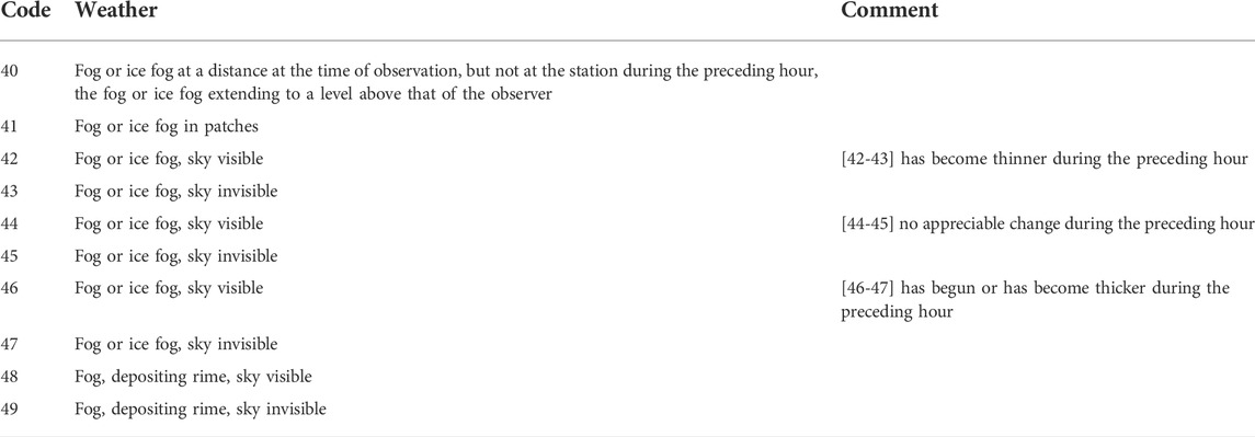
TABLE 1. The present weather code based on SYNOP rules.

To investigate atmospheric circulations during marine fog, we used the fifth-generation reanalysis (ERA5) (Hersbach et al., 2020) provided by the European centre for medium-range weather forecasts (ECMWF). The ERA5 fields are on a 0.25° × 0.25° grid with 12 levels below 700 hPa. The spatial resolution is high enough to depict the large-scale atmospheric circulations and characterize their influence on the MABL (Yang et al., 2018). The time resolution is 1 h; therefore, the ERA5 can match ICOADS hour by hour.

2.2 Methods

Temperature inversions usually cap marine fog and exert a strong influence on the evolution of fog (Cao et al., 2007; Zhang et al., 2009; Yang et al., 2018). Following Cao et al. (2007), we identified the inversions between 1000 hPa and 800 hPa, corresponding approximately to the surface and 2000 m. All vertical profiles were divided into three layers: surface to inversion base, inversion base to inversion top, and inversion top to 800 hPa. We followed the scaling method of Norris (1998) to rescale the composite vertical profiles and capture the characteristics of the MABL.

Turbulence plays an important role in the formation of fog (Koračin et al., 2005; Guo et al., 2015; Huang et al., 2015). The bulk Richardson number (Ri) can be used as a measure of turbulence (Zhang et al., 2008; Huang et al., 2011; Kim and Yum, 2012):

$\mathit{Ri}=\frac{\mathit{g}}{\mathit{\theta }}\frac{\mathrm{\Delta }\mathit{\theta }/\mathrm{\Delta }\mathit{z}}{{\left(\mathrm{\Delta }\mathit{u}/\mathrm{\Delta }\mathit{z}\right)}^2+{\left(\mathrm{\Delta }\mathit{v}/\mathrm{\Delta }\mathit{z}\right)}^2}$

where g is the gravitational constant, z is the reference level, θ is the potential temperature at the reference level, and u and v are the wind components at the reference level. The relative importance of static stability and dynamic instability is expressed by Ri. Arya (1972) proposed a value of 0.25 as the critical value for Ri, above which the air is no longer turbulent and mesoscale motions are important. Furthermore, if Ri > 1, then the air is statically and dynamically stable and no turbulence can occur. If Ri < 0, then the air is both statically unstable and dynamically unstable, and any disturbance can generate turbulence (Galperin et al., 2007).

The Student’s t-test (Wilks, 1996) was applied to assess the statistical significance of the results in the composite analysis.

3 Synoptic background

3.1 Large-scale circulation

The NP weather is controlled by two semipermanent weather systems in winter climatology. One is the Aleutian Low, which brings persistent eastward winds to the midlatitude NCP at 1000 hPa (Figure 2A). Another is the NPSH, whose location shifts from the western to the eastern Pacific compared to summer (Zhang et al., 2015).

FIGURE 2

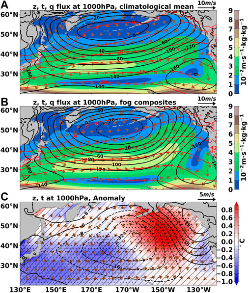
FIGURE 2. (A) Horizontal wind vectors (m·s⁻¹), geopotential height (black contour, gpm), temperature (red contour, °C), and water flux (shaded, in 10⁻²m·s⁻¹·kg·kg⁻¹) at 1000 hPa in winter for the climate state. (B) Same as (A) but for NEP fog composite in winter (C) anomaly for the NEP fog composite: Geopotential height (black contour, in gpm), temperature (shaded, °C), and horizontal wind (vectors, m·s⁻¹). The black dots denote that the temperature anomaly is significant at the 95% confidence level based on the Student’s t-test. The shade lines indicate the geopotential height anomaly significant at the 95% confidence level.

We calculated the composite large-scale circulation corresponding to the NEP fog based on the ERA5 reanalysis (Figure 2B). Results show that the circulation patterns of the fog composites differ from those of the climatological mean state. The area encircled by an isoline of 0 gpm extends southward, indicating a slight southward movement of the low-pressure center of the Aleutian Low. Meanwhile, the area encircled by an isoline of 160 gpm shrinks eastward. Such a circulation configuration contributes to abnormal southerly winds in fog areas. The southerly wind associated with the abnormal low pressure in the NCP carries more warm and moist air northward compared to conditions for the climatological mean state (Figures 2B,C).

Figure 3 shows surface wind rose diagrams based on the observations during NEP fog in winter. Almost all fog events are accompanied by southerly winds, consistent with the circulation pattern.

FIGURE 3

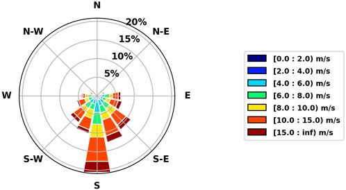
FIGURE 3. Surface wind rose diagrams (%) based on ICOADS observations during NEP fog in winter (1979–2019).

3.2 Air–sea interface

The difference between the surface air temperature (SAT) and the SST was used to represent the stability at the air–sea interface. The air and ocean properties of the narrow coastal region of North America differ from the open ocean westward in general (Figure 4). The SAT–SST anomaly in the offshore area is positive and greater than 0.8°C in most of the NEP fog region, indicating a stable air–sea interface, compared to the climatological mean state whose SAT–SST is negative in the NEP (Figure 4C). The SAT anomaly is positive with an abnormal southerly surface wind (Figure 4A), consistent with the circulation pattern (Figure 2C). The SST anomaly is less than 0.1°C and does not pass the significance test (Figure 4B). This condition indicates that the stable air–sea interface is dominated during these conditions.

FIGURE 4

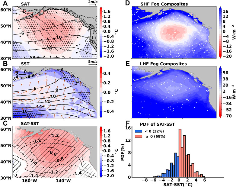
FIGURE 4. Air and ocean properties of the NEP fog. (A) Surface horizontal wind anomaly (vectors, m·s⁻¹), climatological mean SAT (black contour, °C), and SAT anomaly (shaded, °C); the black dots denote that the SAT anomaly is significant at the 95% confidence level. (B) Surface horizontal wind with fog (vectors, m·s⁻¹), climatological SST (black contour, °C), and SST anomaly (shaded, °C); the black dots indicate the SST anomaly significant at the 95% confidence level. (C) Climatological SAT–SST (black dashed contour, °C) and SAT–SST anomaly (shaded, °C); the shade lines indicate the SAT–SST anomaly significant at the 95% confidence level. (D) SHF with fog (shaded, W·m⁻²). (E) LHF with fog (shaded, W·m⁻²). (F) Probability density functions (%) of SAT–SST (°C).

The surface sensible heat flux (SHF) is dominantly downward and the surface latent heat flux (LHF) in the open ocean is upward in fog (Figures 4D,E). The sea surface continuously cools the marine fog as fog forms and develops (Figure 4D). The relatively low upward LHF ($\sim$10 W m⁻²) in most of the fog areas indicates that local moisture supply from the sea surface is suppressed by the moist air from the south, compared to the surrounding area where LHF exceeds 60 W m⁻² (Figure 4E).

The observations show that positive SAT–SST occurs in most fog cases (68%) (Figure 4F), which is consistent with the air–sea interface analysis above.

4 Marine atmospheric boundary layer structure

Both fog and clouds form when water vapor condenses or freezes in the air, forming tiny droplets or crystals. Sometimes they can convert to each other (Petterssen, 1936; Koračin et al., 2001; Kim and Yum, 2013). Figure 5 shows the distinct MABL structures between fog and low clouds over the NEP. For fog, the inversion is found between 925 hPa and 875 hPa with a strength of 0.08 K hPa⁻¹ (Figure 5A), while the inversion for low clouds is weaker (0.06 K hPa⁻¹) with a higher inversion base (900 hPa) (Figure 5C). The slope of the potential temperature (θ) as a function of height is positive for fog, indicating dry adiabatic stability. The θ below 950 hPa increases slightly, indicating a nearly mixing layer from 1000 hPa to 950 hPa in cases of low clouds. The slope of the saturated equivalent potential temperature (${\theta }_{se}$) is slightly negative for both fog and clouds below 975 hPa, indicating a wet adiabatic unstable stratification (Figures 5A,C).

FIGURE 5

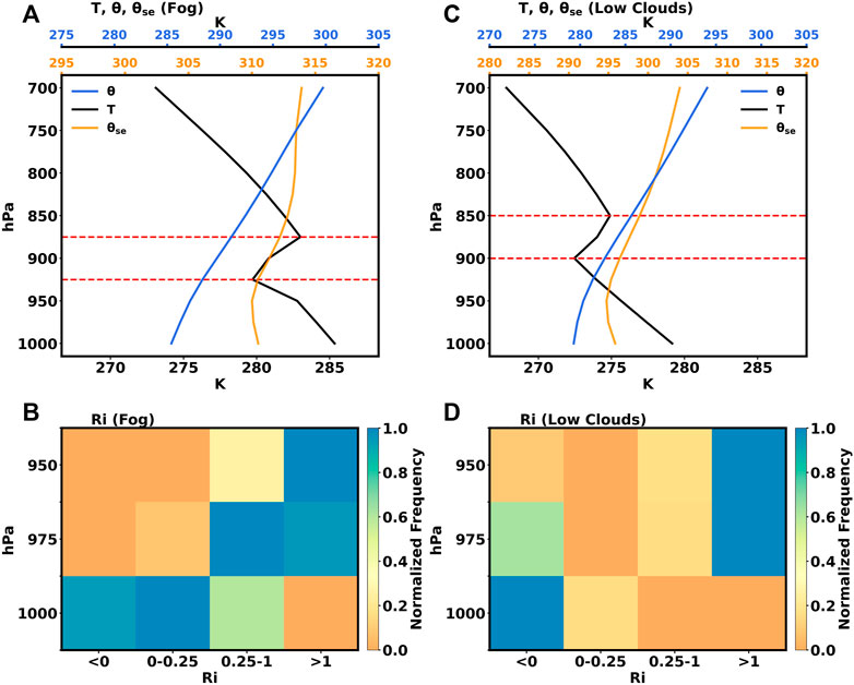
FIGURE 5. Composite profiles and the bulk Richardson number frequency distribution concurrent with fog (A,B) and low clouds (C,D): temperature (T, black line, K), potential temperature $\theta$($\theta$, blue line, K), saturated equivalent potential temperature ${\theta }_{se}$(${\theta }_{se}$, orange line, K), and the bulk Richardson number (Ri, shaded). The red dashed lines denote the inversion layer.

Normalized frequency was used to highlight the differences between Ri ranges. The normalized frequency of an Ri range at a reference level $x^{\text{∗}}$ can be expressed as:

${\mathit{x}}^{\mathit{\ast }}=\frac{\mathit{x}-{\mathit{x}}_{\mathit{min}}}{{\mathit{x}}_{\mathit{max}}-{\mathit{x}}_{\mathit{min}}}$

where $x$ is the frequency of the Ri range, $x_{max}$ is the maximum frequency in all of the Ri ranges, and $x_{min}$ is the minimum frequency in all of the Ri ranges.

The Ri range of maximum frequency below 975 hPa is 0–0.25 for fog, whereas it is less than 0 for low clouds (Figures 5B,D). This indicates that the lower atmosphere is more unstable in cloudy cases compared to fog events, which is because of the unstable air–sea interface associated with the negative SAT–SST (Figure 6B).

FIGURE 6

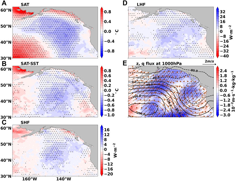
FIGURE 6. Difference between thermodynamic properties for cases of low clouds and fog. (A) SAT (shaded, °C), the black dots indicate the SAT difference significant at the 95% confidence level. (B) SAT–SST (shaded, °C); the black dots indicate the SAT–SST difference significant at the 95% confidence level. (C) SHF (shaded, W·m⁻²); the black dots indicate the SHF difference significant at the 95% confidence level. (D) LHF (shaded, W·m⁻²), the black dots indicate the LHF difference significant at the 95% confidence level. (E) Geopotential height (black contour, gpm), water flux (shaded, 10⁻²m·s⁻¹·kg·kg⁻¹), and horizontal wind (vectors, m/s). The black dots indicate the water flux difference significant at the 95% confidence level. The shaded lines indicate the geopotential height difference significant at the 95% confidence level.

The stability of the lower atmosphere is affected by the air–sea interaction (Cho et al., 2000; Heo and Ha, 2010; Huang et al., 2011; Koračin et al., 2014). We investigate the difference between the air–sea interface with low clouds and fog. The surface air in cases of low clouds is cooler compared to the cases of fog events (Figure 6A). It is the cooler surface air that leads to a negative SAT–SST (Figure 6B) because of the abnormal northwest wind, indicating weaker cooling or stronger warming of the air by the sea surface (Figure 6C). The upward LHF at the surface is greater because of less moist air, which is also related to the abnormal northwest wind (Figures 6D,E). There is a dipole morphology of the geopotential height anomaly with high west and low east, which causes the abnormal northwest wind (Figure 6E).

5 The cause of the negative surface air temperature–sea surface temperature

It is notable that although most SAT–SST is positive during fog, there are approximately 32% of fog cases with a negative SAT–SST (Figure 4F). Fog resulting from the advection of colder air over the warm sea surface is called warm sea fog (Taylor, 1917). This type of fog formation stems from the advection of colder air over the warm sea where saturation occurs in response to the mixing of the cold and sufficiently moist air with warm/moist air (Koračin et al., 2014). Another type of fog associated with a warm sea surface is steam fog, which can occur when a stream of cold, dry air traverses a much warmer sea surface. Steam fog is always associated with extremely large (100s or more of W·m⁻²) sensible and latent heat fluxes (Koračin et al., 2014).

To explore the causes of negative SAT–SST, we show in Figure 7 the differences between fog with negative and positive SAT–SST. The SST difference between the two kinds of fog is less than 0.1°C (Figure 7B). Moreover, both the specific humidity difference at 1000 hPa and the SAT difference between two kinds of fog are not significant in most areas (Figures 7A–C), suggesting that the lower atmosphere condition of fog with negative and positive SAT–SST is generally the same. Thus, these cases should not be considered warm sea fog. Both the SHF and LHF differences are less than 16 W m⁻² (Figures 7D,E), which is not large enough to classify them as the steam fog mentioned above.

FIGURE 7

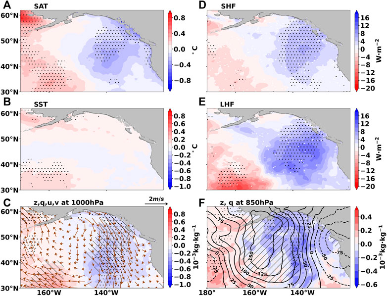
FIGURE 7. Difference between fog with AWSS and that with ACSS. (A) SAT (shaded, °C), the black dots indicate the SAT difference significant at the 95% confidence level. (B) SST (shaded, °C), the black dots indicate the SST difference significant at the 95% confidence level. (C) Horizontal wind (vectors, m·s⁻¹) and specific humidity (shaded, 10⁻³kg kg⁻¹) at 1000 hPa. The black dots indicate the temperature difference significant at the 95% confidence level. Slash lines indicate the geopotential height anomaly significant at the 95% confidence level. Backslashes indicate the meridional wind significant at the 95% confidence level. (D) SHF (shaded, W·m⁻²), and the black dots indicate the SHF difference significant at the 95% confidence level. (E) LHF (shaded, W·m⁻²); the black dots indicate the LHF difference significant at the 95% confidence level. (F) Geopotential height (black contour, gpm) and specific humidity (shaded, 10⁻³kg kg⁻¹) at 850 hPa. The black dots indicate the specific humidity difference significant at the 95% confidence level. The slash lines indicate the geopotential height anomaly significant at the 95% confidence level.

Yang et al. (2018) suggest that approximately 33% of the advection-cooling fog is with negative SAT–SST in the western Yellow Sea. As mentioned above, a similar phenomenon also occurs in the NEP. Under such circumstances, the sea surface can heat the air. Thus, the air–sea interface is divided into two states: air cooling by sea surface (ACSS) and air warming by sea surface (AWSS). The related expressions of “fog with ACSS” and “fog with AWSS” are used to name our fog cases. The different features between them are examined.

Figure 7F shows that for fog with AWSS, there is significantly abnormal high pressure at 850 hPa, suggesting abnormal sinking motion that can enhance thermal and moisture stratification between the MABL and the free atmosphere through adiabatic warming (Yang et al., 2018).

Figure 8 shows the surface wind rose diagrams based on the ICOADS observations during fog with ACSS and AWSS. The southerly wind dominates in both fog types. All the northerly winds occur in fog with AWSS. However, the frequencies and magnitudes are much smaller. The wind field is generally the same for fog with ACSS and fog with AWSS because the abnormal northerly wind is not significant in most areas (Figure 7C).

FIGURE 8

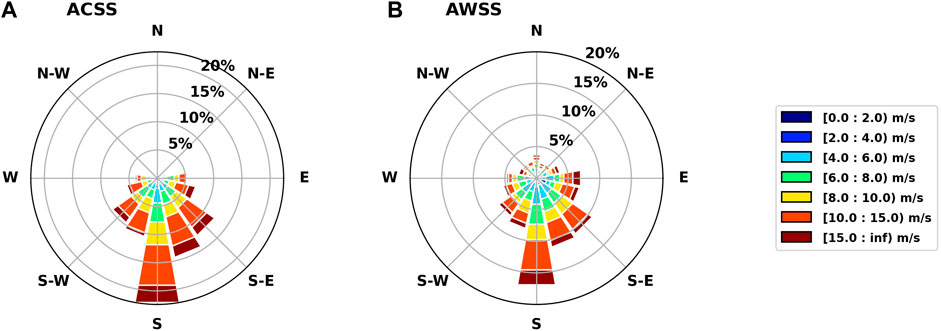
FIGURE 8. Surface wind rose diagrams (%) based on the ICOADS observations during NEP fog in winter (1979–2019). (A) Fog during ACSS. (B) Fog during AWSS.

The MABL structures between fog with ACSS and that with AWSS are also compared (Figure 9). In general, results seem to be similar, but some differences exist. The inversion bottom of fog with AWSS is higher compared to fog with ACSS, indicating that the fog with AWSS may be thicker than fog with ACSS. The intensity of the inversion layer is the same. The slopes of θ as a function of height are both positive, indicating dry adiabatic stability. The ${\theta }_{se}$ profile shows that there are wet adiabatic unstable layers below 950 hPa in both types of fog. The top of the wet adiabatic mixing layer is at approximately 950 hPa for fog with ACSS, but at approximately 925 hPa for fog with AWSS (Figures 9B,D). The relative humidity for fog with AWSS decreases sharply upward beneath the inversion bottom. The relative humidity is approximately 0.7 for fog with AWSS but more than 0.8 for fog with ACSS at their inversion bottoms. It implies that the air is drier above the inversion bottom for fog with AWSS than for fog with ACSS (Figures 9C,F). This enhances longwave radiative cooling at the fog top. The difference between fog with ACSS and that with AWSS also shows that the specific humidity at 850 hPa is significantly low for fog with AWSS (Figure 7F), indicating a wide range of dry layers above the MABL that can enhance longwave radiative cooling.

FIGURE 9

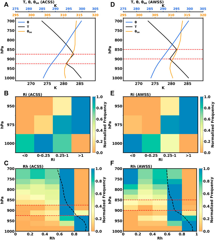
FIGURE 9. Composite profiles, the bulk Richardson number, and relative humidity frequency distribution concurrent with fog with ACSS (A–C) and fog with AWSS (D–F): temperature (T, black line, in K), potential temperature ($\theta$, blue line, in K), saturated equivalent potential temperature (${\theta }_{se}$, orange line, in K), the bulk Richardson number (Ri, shaded), and relative humidity (Rh, shaded). The red dashed lines denote the inversion layer.

Following the method proposed by Yang et al. (2018), the outgoing longwave radiation from the fog top was estimated by the upward longwave radiative flux at the top of atmosphere clouds and the Earth’s radiant energy system. The average top of atmosphere upward longwave fluxes of fog with AWSS are 215 W m⁻², stronger than that of fog with ACSS (208 W m⁻²).

Thus, fog with AWSS likely occurs during the developing and maintaining step of cold sea fog events because of longwave radiation from the fog top and turbulent mixing in the fog layer (Koračin and Dorman, 2017; Yang et al., 2018).

6 Summary and discussions

The present study uses the 40-year ICOADS observations and ERA5 reanalysis results to reveal the synoptic conditions and the MABL structure of marine fog over the NEP in winter. By comparing the climatological mean state and fog composites, it was found that the fog-prone area is controlled by the eastern flank of the Aleutian Low and the northwestern flank of the Pacific subtropical high, which together contribute to a warm and moist northward airflow to form advection-cooling fog over the NEP.

The inversion structure, θ and ${\theta }_{se}$ profiles, and normalized frequency of the Ri were investigated to highlight the distinct MABL structures between fog and low clouds. During fog events, the inversion bottom is at lower elevations (at 925 to 875 hPa) compared to the cloudy cases (at 900 hPa). The inversion strength is greater for fog cases (0.08 K hPa⁻¹) compared to the low-cloud cases (0.06 K hPa⁻¹). The lower atmosphere is more stable during fog cases compared to low-cloud events.

Composite analysis of fog cases shows that atmospheric circulation has the characteristics of advection-cooling fog. It is notable that approximately 32% of fog cases have negative SAT–SST, which cannot be explained by warm advection fog and steam fog. To investigate this phenomenon, the difference between the fog with AWSS and that with ACSS was examined. The results show that for fog with AWSS, the air is drier above the inversion bottom than in cases of fog with ACSS. Dry air contributes to the cooling of the fog layer by enhancing the longwave radiative cooling at the fog top and the vertical mixing beneath, which most probably lead to the negative SAT–SST.

This present study mainly focuses on fog formed over a cooler sea surface which appears most frequently in the NEP. Fog can also occur over warmer sea surfaces under the influence of cooler air advection, such as steam fog and fog associated with stratus lowering (thickening) (Oliver et al., 1978; Pilié et al., 1979; Koračin et al., 2001). These kinds of fog, though less frequent, are likely to appear in winter, which should be analyzed further. On the other hand, it is necessary to conduct numerical simulations and experiments to investigate quantitatively the physical processes in the marine boundary layer and the relationships between fog and low stratus. This will be a focus of a future study.

The longwave cooling at the top of the stratus or fog can create negative buoyancy, causing stratus thickening/lowering (Petterssen, 1936; Koračin et al., 2014). We note that this phenomenon is more closely associated with AWSS than with ACSS over the NEP. In fog with AWSS, the proportion of sinking motion near the LCL is greater than in fog with ACSS (not shown), implying a stronger longwave cooling and negative buoyancy. The sinking motion forced by synoptic-scale weather disturbances should also be considered. The stronger sinking motion indicates that the thickening and lowering of stratus also play a part in the fog with AWSS.

Further studies will also include an investigation of the impact of air–sea interaction, the evolution of the MABL structure, and radiation fluxes on the formation and dissipation of fog as well as on transitions between cloud and fog in the NEP region.

Data availability statement

The original contributions presented in the study are included in the article/Supplementary Material, further inquiries can be directed to the corresponding author.

Author contributions

XL: data analysis; methodology and software; and writing—original draft. SZ: supervision; providing research guidance for this article; and writing—review. DK: giving suggestions and corrections for the manuscript and writing—review. LY and XZ: data curation.

Funding

This work was supported by the National Key Research and Development Program of China (NKPs, 2019YFC1510102 and 2021YFC3101600) and the Natural Science Foundation of China (NSFC, 41876130 and 41975024). DK was supported under project STIM—REI, Contract Number: KK.01.1.1.01.0003, a project funded by European Union through the European Regional Development Fund—Operational Programme Competitiveness and Cohesion 2014-2020 (KK.01.1.1.01). DK was also partially funded by project CAAT (Coastal Auto-purification Assessment Technology) funded by European Union from European Structural and Investment Funds 2014—2020, Contract Number: KK.01.1.1.04.0064. DK also acknowledges significant support from the University of Notre Dame, USA (ONR Grant: N00014-21-1-2296).

Acknowledgments

We thank the management and publishing organizations responsible for the ECMWF ERA5 data and ICOADS data.

Conflict of interest

The authors declare that the research was conducted in the absence of any commercial or financial relationships that could be construed as a potential conflict of interest.

Publisher’s note

All claims expressed in this article are solely those of the authors and do not necessarily represent those of their affiliated organizations, or those of the publisher, the editors, and the reviewers. Any product that may be evaluated in this article, or claim that may be made by its manufacturer, is not guaranteed or endorsed by the publisher.

References

Arya, S. (1972). The critical condition for the maintenance of turbulence in stratified flows. Q. J. R. Meteorol. Soc. 98 (416), 264–273. doi:10.1002/qj.49709841603

CrossRef Full Text | Google Scholar

Cao, G., Giambelluca, T. W., Stevens, D. E., and Schroeder, T. A. (2007). Inversion variability in the Hawaiian trade wind regime. J. Clim. 20 (7), 1145–1160. doi:10.1175/jcli4033.1

CrossRef Full Text | Google Scholar

Cho, Y.-K., Kim, M.-O., and Kim, B.-C. (2000). Sea fog around the Korean Peninsula. J. Appl. Meteor. 39 (12), 2473–2479. doi:10.1175/1520-0450(2000)039<2473:sfatkp>2.0.co;2

CrossRef Full Text | Google Scholar

Dorman, C. E., Mejia, J., Koračin, D., and McEvoy, D. (2017). “Worldwide marine fog occurrence and climatology,” in Marine fog: Challenges and advancements in observations, modeling, and forecasting (Springer), 7–152.

CrossRef Full Text | Google Scholar

Fu, G., and Song, Y. J. (2014). Climatology characteristics of sea fog frequency over the Northern Pacific. J. Ocean Univ. China. 44 (10), 35–41.

Google Scholar

Galperin, B., Sukoriansky, S., and Anderson, P. S. (2007). On the critical Richardson number in stably stratified turbulence. Atmos. Sci. Lett. 8 (3), 65–69. doi:10.1002/asl.153

CrossRef Full Text | Google Scholar

Gao, S., Lin, H., Shen, B., and Fu, G. (2007). A heavy sea fog event over the Yellow Sea in March 2005: Analysis and numerical modeling. Adv. Atmos. Sci. 24 (1), 65–81. doi:10.1007/s00376-007-0065-2

CrossRef Full Text | Google Scholar

Gultepe, I., Tardif, R., Michaelides, S., Cermak, J., Bott, A., Bendix, J., et al. (2007). Fog research: A review of past achievements and future perspectives. Pure Appl. Geophys. 164 (6), 1121–1159. doi:10.1007/s00024-007-0211-x

CrossRef Full Text | Google Scholar

Guo, J., Li, P., Fu, G., Zhang, W., Gao, S., Zhang, S., et al. (2015). The structure and formation mechanism of a sea fog event over the Yellow Sea. J. Ocean. Univ. China 14 (1), 27–37. doi:10.1007/s11802-015-2466-7

CrossRef Full Text | Google Scholar

Heo, K.-Y., and Ha, K.-J. (2010). A coupled model study on the formation and dissipation of sea fogs. Mon. Weather Rev. 138 (4), 1186–1205. doi:10.1175/2009mwr3100.1

CrossRef Full Text | Google Scholar

Hersbach, H., Bell, B., Berrisford, P., Hirahara, S., Horányi, A., Muñoz‐Sabater, J., et al. (2020). The ERA5 global reanalysis. Q. J. R. Meteorol. Soc. 146, 1999–2049. doi:10.1002/qj.3803

CrossRef Full Text | Google Scholar

Huang, H., Liu, H., Jiang, W., Huang, J., and Mao, W. (2011). Characteristics of the boundary layer structure of sea fog on the coast of southern China. Adv. Atmos. Sci. 28 (6), 1377–1389. doi:10.1007/s00376-011-0191-8

CrossRef Full Text | Google Scholar

Huang, H., Liu, H., Huang, J., Mao, W., and Bi, X. (2015). Atmospheric boundary layer structure and turbulence during sea fog on the southern China coast. Mon. Weather Rev. 143 (5), 1907–1923. doi:10.1175/mwr-d-14-00207.1

CrossRef Full Text | Google Scholar

Johnstone, J. A., and Mantua, N. J. (2014). Atmospheric controls on northeast Pacific temperature variability and change, 1900–2012. Proc. Natl. Acad. Sci. U. S. A. 111 (40), 14360–14365. doi:10.1073/pnas.1318371111

PubMed Abstract | CrossRef Full Text | Google Scholar

Kalnay, E., Kanamitsu, M., Kistler, R., Collins, W., Deaven, D., Gandin, L., et al. (1996). Bull. Am. Meteorol. Soc. 77 (3), 437–471. doi:10.1175/1520-0477(1996)077<0437:tnyrp>2.0.co;2

CrossRef Full Text

Kim, C. K., and Yum, S. S. (2012). Marine boundary layer structure for the sea fog formation off the west coast of the Korean Peninsula. Pure Appl. Geophys. 169 (5), 1121–1135. doi:10.1007/s00024-011-0325-z

CrossRef Full Text | Google Scholar

Kim, C. K., and Yum, S. S. (2013). A study on the transition mechanism of a stratus cloud into a warm sea fog using a single column model PAFOG coupled with WRF. Asia. Pac. J. Atmos. Sci. 49 (2), 245–257. doi:10.1007/s13143-013-0024-z

CrossRef Full Text | Google Scholar

Koračin, D., Lewis, J., Thompson, W. T., Dorman, C. E., and Businger, J. A. (2001). Transition of stratus into fog along the California coast: Observations and modeling. J. Atmos. Sci. 58 (13), 1714–1731. doi:10.1175/1520-0469(2001)058<1714:tosifa>2.0.co;2

CrossRef Full Text | Google Scholar

Koračin, D., Businger, J. A., Dorman, C. E., and Lewis, J. M. (2005). Formation, evolution, and dissipation of coastal sea fog. Bound. Layer. Meteorol. 117 (3), 447–478. doi:10.1007/s10546-005-2772-5

CrossRef Full Text | Google Scholar

Koračin, D., Dorman, C. E., Lewis, J. M., Hudson, J. G., Wilcox, E. M., Torregrosa, A., et al. (2014). Marine fog: A review. Atmos. Res. 143, 142–175. doi:10.1016/j.atmosres.2013.12.012

CrossRef Full Text | Google Scholar

Koračin, D., and Dorman, C. E. (2017). “Marine fog: Challenges and advancements in observations and forecasting.,” Springer Atmospheric Sciences Series (Cham, Switzerland: Springer International Publishing), 537. doi:10.1007/978-3-319-45229-6

CrossRef Full Text | Google Scholar

Lewis, J., Koračin, D., Rabin, R., and Businger, J. (2003). Sea fog off the California coast: Viewed in the context of transient weather systems. J. Geophys. Res. 108 (D15), 4457. doi:10.1029/2002jd002833

CrossRef Full Text | Google Scholar

Norris, J. R. (1998). Low cloud type over the ocean from surface observations. Part I: Relationship to surface meteorology and the vertical distribution of temperature and moisture. J. Clim. 11 (3), 369–382. doi:10.1175/1520-0442(1998)011<0369:lctoto>2.0.co;2

CrossRef Full Text | Google Scholar

Oliver, D., Lewellen, W., and Williamson, G. (1978). The interaction between turbulent and radiative transport in the development of fog and low-level stratus. J. Atmos. Sci. 35 (2), 301–316.

Google Scholar

Petterssen, S. (1936). On the causes and the forecasting of the California fog. J. Aeronaut. Sci. 3 (9), 305–309. doi:10.2514/8.246

CrossRef Full Text | Google Scholar

Pilié, R. J., Mack, E. J., Rogers, C. W., Katz, U., and Kocmond, W. C. (1979). The Formation of marine fog and the development of fog-stratus systems along the California coast. J. Appl. Meteor. 18, 1275–1286. doi:10.1175/1520-0450(1979)018<1275:tfomfa>2.0.co;2

CrossRef Full Text | Google Scholar

Sugimoto, S., Sato, T., and Nakamura, K. (2013). Effects of synoptic-scale control on long-term declining trends of summer fog frequency over the Pacific side of Hokkaido Island. J. Appl. Meteorol. Climatol. 52 (10), 2226–2242. doi:10.1175/jamc-d-12-0192.1

CrossRef Full Text | Google Scholar

Taylor, G. (1917). The formation of fog and mist. Q. J. R. Meteorol. Soc. 43 (183), 241–268. doi:10.1002/qj.49704318302

CrossRef Full Text | Google Scholar

Wang, B. (1985). Sea fog. Beijing: China Ocean Press.

Google Scholar

Wilks, D. S. (1996). Statistical methods in the atmospheric sciences. San Diego, CA: Academic Press.

Google Scholar

WMO (2009). WMO-No. 306, manual on codes.[Online]. International Codes, Vol. I.1. Available at: http://marswiki.jrc.ec.europa.eu/agri4castwiki/images/a/ad/WMO_306_VolI1_en.pdf (Accessed August 8, 2020).

Google Scholar

Woodruff, S. D., Worley, S. J., Lubker, S. J., Ji, Z., Eric Freeman, J., Berry, D. I., et al. (2011). ICOADS release 2.5: extensions and enhancements to the surface marine meteorological archive. Int. J. Climatol. 31 (7), 951–967. doi:10.1002/joc.2103

CrossRef Full Text | Google Scholar

Xia, L., Tan, Y., Li, C., and Cheng, C. (2016). The classification of synoptic-scale eddies at 850 hPa over the North Pacific in wintertime. Adv. Meteorol. 2016, 1–8. doi:10.1155/2016/4797103

CrossRef Full Text | Google Scholar

Yang, L., Liu, J. W., Ren, Z. P., Xie, S. P., Zhang, S. P., Gao, S. H., et al. (2018). Atmospheric conditions for advection‐radiation fog over the Western Yellow Sea. J. Geophys. Res. Atmos. 123 (10), 5455–5468. doi:10.1029/2017jd028088

CrossRef Full Text | Google Scholar

Zhang, S., Ren, Z., Liu, J., Yang, Y., and Wang, X. (2008). Variations in the lower level of the PBL associated with the Yellow Sea fog-new observations by L-band radar. J. Ocean. Univ. China 7 (4), 353–361. doi:10.1007/s11802-008-0353-1

CrossRef Full Text | Google Scholar

Zhang, S.-P., Xie, S.-P., Liu, Q.-Y., Yang, Y.-Q., Wang, X.-G., Ren, Z.-P., et al. (2009). Seasonal variations of Yellow sea fog: Observations and mechanisms. J. Clim. 22 (24), 6758–6772. doi:10.1175/2009jcli2806.1

CrossRef Full Text | Google Scholar

Zhang, S., Chen, Y., Long, J., and Han, G. (2015). Interannual variability of sea fog frequency in the Northwestern Pacific in July. Atmos. Res. 151, 189–199. doi:10.1016/j.atmosres.2014.04.004

CrossRef Full Text | Google Scholar