Application of high-resolution processing in seismic data based on an improved synchrosqueezing transform

Highlights

1) A new high-resolution processing technique for seismic data.

2) The improved synchrosqueezing transform based on the generalized Fourier transform.

3) The phase correction value is calculated using the instantaneous frequency of seismic data.

4) Both synthetic signal and actual data results show remarkable improvement.

5) The new method has a good application prospect in resource exploration.

1 Introduction

With the deepening of exploration and development of oil and gas fields, exploration and development are becoming increasingly difficult. Considering that seismic signals are typical non-stationary signals in nature, the time–frequency analysis technology in modern signal processing can obtain the change process of seismic signals in the time and frequency domains at the same time and extract effective time–frequency characteristics for lithology and fluid interpretation. This study proposes a time–frequency analysis method to improve the time–frequency resolution of seismic data (Li et al., 2004; Wu and Liu, 2009; Han and Van der Baan, 2013).

At present, Fourier transform (FT) is still the most commonly used time–frequency transform method in signal analysis. With the gradual deepening of research on non-stationary signals, researchers have proposed a series of signal analysis techniques aimed at the problems existing in FT, among which the short-time Fourier transform (STFT) (Potter and Steinberg, 1950; Potter et al., 1966) and wavelet transform (WT) (Morlet et al., 1982a; 1982b) are the two primary methods (Abry et al., 1993; Sinha et al., 2005; Daubechies, 2004; Gao et al., 2006; Chen and Gao, 2007). In order to improve the time–frequency resolution of STFT, Kodera et al. (1976) first proposed the time–frequency spectrum rearrangement technique and later generalized it to any bilinear time–frequency or time-scale representation by Auger and Flandrin (1995). Since this method has no accurate inverse transformation, mathematically, it did not receive widespread attention in the years soon after its development. Recently, with the increasing difficulty of exploration and development, the time–frequency spectrum rearrangement method has attracted extensive attention in the field of seismic exploration (Odegard et al., 1997; Han, 2013; Shang, 2014; Kahoo and Siahkoohi, 2009; Pedersen et al., 2003).

The synchrosqueezing transform (SST) is similar to the time–frequency spectrum rearrangement method, which was proposed by Daubechies et al. (2011). In essence, it recalculates a position close to the real coordinates of the time–frequency energy spectrum so as to rearrange the energy according to it. In recent years, SST has been applied in the rearrangement of various original time–frequency representations, including the continuous wavelet transform (CWT) (Daubechies et al., 2011), wave packet transforms (Wang and Gao, 2017), STFT (Oberlin et al., 2014), S transform (Huang et al., 2016), and generalized S transform (Wang et al., 2018). In addition, some new techniques based on the notion of the SST have been proposed, such as the high-order synchrosqueezed transform (Liu W. et al., 2018), concentration of frequency and time (ConceFT) (Daubechies et al., 2016), synchroextracting transform (Yu et al., 2017), and others (Li and Liang, 2012; Thakur et al., 2013; Liu N. et al., 2018; Xue et al., 2019).

Most of the abovementioned methods have been used in seismic signal processing (Huang et al., 2016; Wang and Gao, 2017; Wang et al., 2018). In addition to this, Herrera et al. (2014) applied the SST to time–frequency analysis of seismic signals for the first time and compared it with CWT and complete ensemble empirical mode decomposition (CEEMD) in detail, which verified the superiority of this method in the time–frequency analysis of seismic signals. Herrera et al. (2015) adopted the technology of P- and S-wave separation based on the SST and verified the method through an example. Siahsar et al. (2016) developed a random noise elimination technique based on the SST and verified the effectiveness of the algorithm through a test case as well. The SST based on the STFT was introduced in seismic data analysis by Wu and Zhou (2018). The method reassigns the STFT values to different points to produce a concentrated time–frequency map.

In these studies, Li and Liang (2012) found that the resolution of the SST could be further improved by adding a phase factor to the traditional SST process via the notion of the generalized Fourier transform (GFT). For signals whose frequency content changes rapidly with time, this method can increase the resolution in order to identify the time–frequency distribution characteristics. Therefore, this method may provide an opportunity for improving the processing of seismic data through time–frequency analysis techniques. The key to this method is obtaining the phase factor, which is related to the instantaneous frequency of the signal. For stationary signals, the instantaneous frequency is a constant, while for non-stationary signals, the instantaneous frequency is a function of time t. As a seismic wave propagates in the underground medium, energy absorption, attenuation, and scattering occur, leading to a complicated time–frequency relationship in seismic waves. Therefore, accurately obtaining the instantaneous frequency of actual seismic data is key to high-resolution processing in the field of petroleum exploration.

In this study, we attempted to calculate the phase factor using the instantaneous frequency of seismic data, extracted by using a complex signal analysis technique based on the Hilbert transform, and present a high-resolution processing technique for seismic data based on the improved SST. In order to prove the feasibility of this approach, synthetic 1D- and 2D-models and actual seismic data from the Tuha Basin, in the Xinjiang autonomous region of China, were tested as an example. This study is divided into five sections. Section 1 contains the introductory content; Section 2 describes the theory and method of the improved SST; Sections 3 and 4 show the calculation results for the method to model data and real seismic data; and Section 5 discusses the results.

2 Materials and methods

The approach proposed in this study is to adjust the frequency change rate of a signal by some reversible means and map it to a specific frequency, ω0, before performing the SST. In order to achieve the aforementioned process, it is necessary to find a reversible transformation, which can have a certain influence on the frequency change rate of the signal but will not affect the accuracy of the time spectrum or the effect of the inverse transformation. We attempted to obtain the phase factor using the instantaneous frequency of seismic data, extracted by a complex signal analysis technique based on the Hilbert transform. In the following sections, we briefly describe the theory of SST and GFT and illustrate the improved SST proposed in this study.

2.1 Brief recap of the SST and GFT

The CWT of a signal s(t) is (Daubechies and Maes, 1996)

$W_s(a,b)={\displaystyle \int s\left(t\right)\frac{1}{\sqrt{a}}}{\psi }^{\ast }\left(\frac{t-b}{a}\right)dt,(1)$

where ${\psi }^{\ast }$ is the complex conjugate of the mother wavelet, and $b$ is a time shift factor, which is scaled by $a$. According to the scaling and shifting method, the signal is analyzed at a multi-scale by the CWT (Kahoo and Siahkoohi, 2009).

Based on Parseval’s theorem in the Fourier domain, the CWT of a signal s(t) can be rewritten into the expression of the frequency domain as follows:

$W_s(a,b)=\frac{1}{2\pi }{\displaystyle \int S\left(\xi \right)\sqrt{a}}{\mathrm{\Psi }}^{\ast }\left(a\xi \right)\exp \left(ib\xi \right)d\xi .(2)$

In order to facilitate the derivation, the seismic signal is assumed to be only a harmonic wave $s\left(t\right)=A\cos \left(\omega t\right)$. The Fourier pair $S\left(\xi \right)=\pi A\left[\delta (\xi -\omega )+\delta (\xi +\omega )\right]$ can be inserted into Eq. 2 as follows:

$\begin{array}{l}{W}_s(a,b)=\frac{A}{2}\sqrt{a}{\displaystyle \int \left[\delta (\xi -\omega )+\delta (\xi +\omega )\right]}{\mathrm{\Psi }}^{\ast }\left(a\xi \right)\exp \left(ib\xi \right)d\xi \\ =\frac{A}{2}\sqrt{a}{\mathrm{\Psi }}^{\ast }\left(a\omega \right)\exp \left(ib\omega \right).\end{array}(3)$

Theoretically, if the FT coefficient of the wavelet ${\Psi }^{\ast }\left(\xi \right)$ is concentrated around the central frequency $\xi ={\omega }_0$, then $W_s(a,b)$ will be concentrated around the scale $a={\omega }_0/\omega$. However, in practice, the energy of the wavelet coefficients often diffuses along the scale $a$ direction, which generates the smearing effect in the time–frequency representation (Daubechies et al., 2011). Daubechies and Maes (1996) found that smearing has little effect along the time $b$ axis. For this reason, the instantaneous frequency ${\omega }_s(a,b)$ can be calculated by taking the partial derivatives for all $W_s(a,b)\ne 0$:

${\omega }_s(a,b)=-i{\left(W_s(a,b)\right)}^{-1}\frac{\partial }{{\partial }_b}{W}_s(a,b).(4)$

Eq. 4 expresses the mapping between the time-scale and time–frequency domains, i.e., $(b,a)\to (b,{\omega }_s(a,b))$. Every point $(b,a)$ can be mapped to $(b,{\omega }_s(a,b))$ using this equation. If the sum of every wavelet coefficient at point $(b,a)$ is converted to $(b,{\omega }_s(a,b))$, the smearing problem can be improved. Because $a$ and $b$ are discrete values, we can define a scale step ${\left(\mathrm{\Delta }a\right)}_k=a_k-a_{k-1}$ and frequency step ${\left(\mathrm{\Delta }w\right)}_k=w_k-w_{k-1}$. Therefore, the time–frequency spectrum after SST is expressed as follows:

$T_s({\omega }_l,b)={\left(\mathrm{\Delta }\omega \right)}^{-1}{\displaystyle \sum _{a_k:\left|\omega (a_k,b)-{\omega }_l\right|<\mathrm{\Delta }\omega /2}{W}_s(a_k,b)a_k^{-3/2}{\left(\mathrm{\Delta }a\right)}_k},(5)$

Eq. 5 is the new time–frequency representation of the signal $T_s(a_l,b)$ according to synchrosqueezing along the frequency axis only (Li and Liang, 2012). The inverse transformation of the SST can be obtained by integrating both sides of Eq. 2 as follows:

$\begin{array}{l}{\displaystyle \underset{0}{\overset{\infty }{\int }}{W}_s(a,b)a^{-3/2}da}=\frac{1}{2\pi }{\displaystyle \underset{-\infty }{\overset{\infty }{\int }}{\displaystyle \underset{0}{\overset{\infty }{\int }}S\left(\xi \right){\mathrm{\Psi }}^{\ast }\left(a\xi \right)\exp \left(ib\xi \right)a^{-1}dad\xi }}\\ =\left({\displaystyle \underset{0}{\overset{\infty }{\int }}{\mathrm{\Psi }}^{\ast }\left(a\xi \right)\frac{d\xi }{\xi }}\right)\text{∗}\left(\frac{1}{2\pi }{\displaystyle \underset{0}{\overset{\infty }{\int }}S\left(\xi \right)\exp \left(ib\xi \right)d\xi }\right).\end{array}(6)$

By taking $C_{\phi }={\displaystyle \int {\mathrm{\Psi }}^{\ast }\left(\xi \right)}\frac{d\xi }{\xi }$, the inverse transformation of the SST can be obtained as follows:

$s\left(t\right)=\mathrm{Re}\left[C_{\phi }^{-1}{\displaystyle \sum _l{T}_s({\omega }_l,b)}\mathrm{\Delta }\omega \right].(7)$

This study adopts a generalized Fourier transform to complete the aforementioned process. The GFT of a signal s(t) is expressed as follows (Detka and El-Jaroudi, 1996):

$S_G\left(\omega \right)={\displaystyle \underset{-\infty }{\overset{+\infty }{\int }}s\left(t\right)\exp (-j2\pi (\omega t+x_0\left(t\right)))dt},(8)$

where $x_0\left(t\right)$ is a real-valued function of $t$, which is used to represent the phase change of the signal. On expanding this equation, it can be found that the GFT of $s\left(t\right)$ is equivalent to the standard FT of $s\left(t\right)\exp (-j2\pi x_0\left(t\right))$. Therefore, the inverse GFT of $S_G\left(\omega \right)$ is

$s\left(t\right)=\exp \left(j2\pi x_0\left(t\right)\right){\displaystyle \underset{-\infty }{\overset{+\infty }{\int }}{S}_G\left(\omega \right)\exp \left(j2\pi \omega t\right)d\omega }.(9)$

By taking $S_G\left(\omega \right)=\delta (\omega -{\omega }_0)$, Eq. 9 can be rewritten as $s\left(t\right)=\exp \left(i2\pi ({\omega }_{0}t+x_0\left(t\right))\right)$. It can be found that signal $s\left(t\right)$ can be mapped to a specific point ${\omega }_0$ through GFT, and the instantaneous frequency of the signal $s\left(t\right)$ is

$\omega \left(t\right)={\omega }_0+\frac{d{x}_0\left(t\right)}{dt}.(10)$

Eq. 10 shows that the key to mapping the instantaneous frequency $\omega \left(t\right)$ of the original signal to the specific frequency ${\omega }_0$ is to determine the function $x_0\left(t\right)$.

2.2 Improved SST for seismic data

In this study, ${\omega }_0$ is the dominant frequency of input data.

Based on the aforementioned expressions, we introduced GFT into the SST and provided the detailed derivation process. The improved SST needs to be calculated in a complex domain. First, the real value signal needs to be transformed into an analytical signal using a Hilbert transform (HT):

$p\left(t\right)=s\left(t\right)+iH\left(s\left(t\right)\right).(11)$

According to Eq. 10, $x_0\left(t\right)$ is calculated based on the instantaneous frequency $\omega \left(t\right)$ of the actual input data. The instantaneous frequency is mathematically defined as the derivative of the signal phase. Taner et al. (1979) introduced a complex signal analysis technique into seismic data processing for the first time and proposed the instantaneous attribute with geological significance. The instantaneous frequencies are extracted by complex signal analysis via the Hilbert transform, which is a signal-value function with time as the variable. The instantaneous frequency is expressed as follows:

${\omega }_n=\frac{\mathrm{d}}{\mathrm{d}t}\left(\arctan \frac{\tilde{s}\left(t\right)}{s\left(t\right)}\right),t=u_n,(12)$

where $\tilde{s}\left(t\right)$ is the Hilbert transform result of the actual seismic data $s\left(t\right)$, and $u_n$ represents the time point corresponding to the maximum envelope of the complex signal. Furthermore, the following calculation was completed:

$q\left(t\right)=p\left(t\right)\exp (-i2\pi x_0\left(t\right)).(13)$

Since $x_0\left(t\right)$ is the function that controls the phase change of the original signal $s\left(t\right)$, the instantaneous frequency of the analytical signal $q\left(t\right)$ does not change significantly with time during the whole period using Eq. 13. In order to reduce the negative frequency effect of $q\left(t\right)$, it is necessary to perform HT on it, as expressed using the following equation:

$r\left(t\right)=q\left(t\right)+iH\left(q\left(t\right)\right).(14)$

According to SST’s implementation steps, CWT of $r\left(t\right)$ is performed. Furthermore, the CWT coefficient of the original signal can be obtained using the following equation:

$W_z(a,b)=W_r(a,b)\exp \left(i2\pi x_0\left(t\right)\right),(15)$

where $W_r(a,b)$ is the CWT of $r\left(t\right)$. According to Eq. 4, we can observe that ${\omega }_s(a,b)={\omega }_z(a,b)$, which means that the instantaneous frequency of $W_z(a,b)$ obtained after the aforementioned processing is consistent with that calculated using the original data.

According to Eq. 14, the moduli of $W_z(a,b)$ and $W_r(a,b)$ are equal; therefore, the aforementioned processing does not change the energy of the original signal. Based on Eq. 14, the SST of $s\left(t\right)$, $T_y({\omega }_l,b)$ can be obtained by processing $W_z(a,b)$ in Eq. 5. This processing of the SST will allow the transfer of $r\left(t\right)$ features to their results, and $r\left(t\right)$ itself is obtained by HT and phase-related processing; therefore, the transmission of the features of $r\left(t\right)$ can achieve the purpose of improving the SST. In essence, the aforementioned processing allows the adjustment of the signal phase before and after the transformation so that it does not affect the expression of the inverse SST. Therefore, the improved inverse SST using the proposed method can be expressed as follows:

$s\left(t\right)=\mathrm{Re}\left[C_{\phi }^{-1}{\displaystyle \sum _l{T}_y({\omega }_l,b)}\mathrm{\Delta }\omega \right].(16)$

3 Results

3.1 1-D synthetic data

In this section, we present how, in order to test the feasibility of the improved method, the improved SST was performed on the cosine non-stationary model (Figures 2A,B) and compared it with the CWT-based SST results (Figure 1D).

FIGURE 1

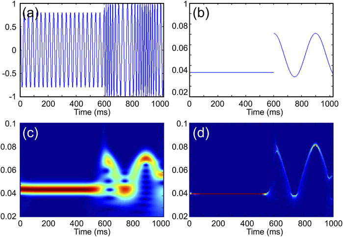
FIGURE 1. Examples of time–frequency representations of the continuous wavelet transform (CWT) and synchrosqueezing transform (SST). (A) Signal s(t)= s₁(t) +s₂(t) is defined by s₁(t) = 0.7cos(πt/15) for 0 ≤ t ≤ 600 ms and by s₂(t) = cos(πt/10+2πsin(πt/150)) for 601 ≤ t ≤ 1,024 ms; (B) instantaneous frequency for its two components (left), ω(t) = 1/30 for 0 ≤ t ≤ 600 ms and ω(t) = (π/10+2πcos(πt/150)*(π/150))/(2π); (C) example of a continuous wavelet transform of s(t), with a Morlet wavelet [this is plotted with MATLAB, with the “jet” colormap; red indicates higher amplitude]; and (D) example of the synchrosqueezing transform(SST) (this is plotted with MATLAB, with the “jet” colormap; red indicates higher amplitude).

We constructed a non-stationary cosine signal. The signal was a stable frequency cosine wave in the range of 0–600 ms and a modulated signal whose frequency varied with the cosine wave in the range of 600–1,000 ms. Figure 1A displays this signal in the time domain, and its theoretical frequency is shown in Figure 1B. Figures 1Cand D illustrate the CWT and SST of the signal, respectively.

It can be seen from Figures 1C,D that the energy focus of CWT is poor and that energy cluster bonding occurs in some places. The SST obviously has higher focusing ability and time–frequency resolution. After further observation, it is not difficult to recognize that the time-frequency spectrum of SST is close to the theoretical frequency of the signal in the range of 0–560 ms. However, in the area of frequency mutation, i.e., around 600 ms, it cannot effectively distinguish between the two very different frequencies but shows a certain smoothing trend. However, the CWT has a better effect at the frequency mutation, showing no smoothness and a real frequency jump. Similarly, when the signal frequency changes at 600–1,000 ms, the energy of SST still diverges slightly in the scale direction.

As shown in Figure 2A, the improved SST effectively reduced the smearing effect of energy on the time axis at the frequency fluctuation, especially at the frequency mutation near 600 ms, which is closer to the theoretical time spectrum than the method in Figure 1. Figure 2B shows the waveform comparison between the original signal and the reconstructed signal. The blue color indicates the original waveform, and the red color indicates the reconstructed data using the inverse transform of the improved SST. The improved SST can reconstruct the model signal accurately without affecting its inverse transformation effect and thus provides a new technical method for threshold denoising in the time–frequency domain and seismic signal reconstruction.

FIGURE 2

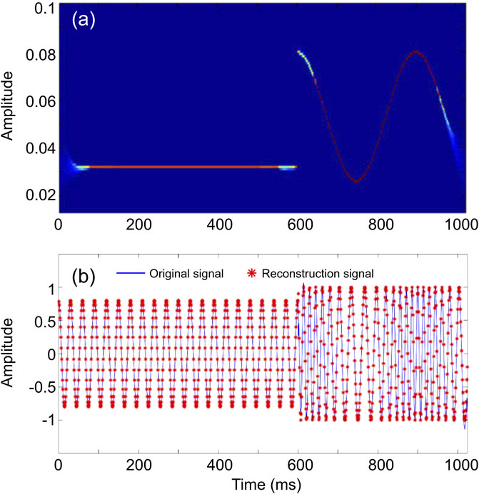
FIGURE 2. Results of the improved synchrosqueezing transform (SST) of s(t), shown in Panel 1. (A) Results of the improved SST for the signal (this is plotted with MATLAB, with the “jet” colormap; red indicates higher amplitude); (B) comparison between the original signal and reconstructed signal by the improved SST [this is plotted with MATLAB, the blue solid line represents the original signal s(t); the red asterisk represents the reconstructed signal].

The frequency component of the model is relatively simple compared with actual data; therefore, we further tested the improved method with irregular synthetic data, which is more similar to the real seismic data (Figure 3A). The synthetic trace in Figure 3A is composed of a set of Morlet wavelets with different frequencies, amplitudes, scales, and time delays.

FIGURE 3

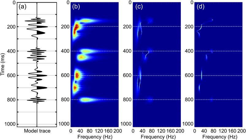
FIGURE 3. Application of the synthetic seismic trace. (A) Original synthetic seismic trace with noise; the signal is composed of two 20 Hz zero-phase Morlet wavelets, with scale = 1 at 250 and 700 ms; two 30 Hz zero-phase Morlet wavelets, with scale = 2 at 200 and 600 ms; three 50 Hz Morlet wavelets, with phase = π/2 and scale = 2 at 150, 400, and 800 ms; and a 40 Hz Morlet wavelet, with phase = π/2 and scale = 2 at 450 ms; (B) time–frequency spectra of synthetic seismic trace using the continuous wavelet transform (CWT); (C) time–frequency spectra of the synthetic seismic trace using the CWT-based synchrosqueezing transform (SST); and (D) time–frequency spectra of synthetic seismic trace using our improved SST. [(B–D) are plotted with MATLAB, with the “jet” colormap; red indicates higher amplitude].

Figures 3B–D show the time–frequency map of CWT, SST, and improved SST, respectively, with the same color scale. Although CWT can recognize the signal components in different frequency bands, the resolution of the time spectrum was obviously insufficient. The distribution of energy groups was not concentrated, and many high-frequency interference components existed (Figure 3B). The results of SST were greatly improved from those of CWT, and the energy distribution was clearly more concentrated. However, it is not difficult to see that if the signal components of two different frequencies are close in time; their time spectra will be entangled with each other, such as at 400–600 ms, or false frequency components will appear. For example, the wavelet frequency of 30 Hz near 600 ms (approximately 550 ms–650 ms) in the time domain extends to nearly 800 ms in the time–frequency representation, and the energy is not concentrated near 600 ms (Figure 3C). The improved SST (Figure 3D) had the best time–frequency focusing effect and could better identify the time–frequency distribution characteristics of the signal. Specifically, the two wavelets at 400 and 450 ms can be more clearly identified on the time spectrum without entanglement. The energy groups of the two sub-waves at 600 and 700 ms were remarkably more concentrated and more easily identified in the time spectrum.

3.2 2-D horizontal layered model

In this section, to test the lateral resolution and the sensitivity of the proposed improved SST in detecting thin reservoirs, we first applied the improved SST to a 2-D horizontal layered model and compared the results to those of the CWT, CWT-based SST (Daubechies et al., 2011), and improved SST methods. The model designed in Figure 4A consisted of five horizontal layers; the third layer was a thin reservoir with a thickness of 10 m, in which, three gas layers with large transverse width variations were developed. The widths of the layers from left to right were 600, 300, and 200 m, respectively. The specific design parameters are shown in Table 1. The geological model was forward modeled with a 30 Hz zero-phase Ricker wavelet. Figure 4B is the pre-stack time migration profile by forward modeling. It can be seen from the migration profile that although a depression existed in the in-phase axis at the gas-bearing location, the presence of fluid cannot be confirmed.

FIGURE 4

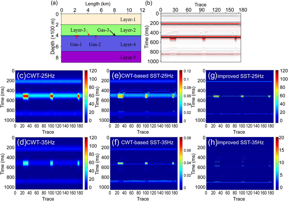
FIGURE 4. Application of the 2-D horizontal model and analysis of the instantaneous frequency used the isofrequency section. (A) Forward model with horizontal layers. The third layer contains three gas layers with large transverse width variations. Model data are created by using the Tesseral 2-D; (B) pre-stack time migration profile of the 2-D forward model. (C) 25 Hz-isofrequency section of the continuous wavelet transform (CWT); (D) 35 Hz-isofrequency section of the CWT; (E) 25 Hz-isofrequency section of the CWT-based SST; (F) 35 Hz-isofrequency section of the CWT-based SST; (G) 25 Hz-isofrequency section of the improved synchrosqueezing transform (SST) in this study; (H) 35 Hz-isofrequency section of the improved SST (these are all plotted with MATLAB, with the “jet” colormap; red indicates higher amplitude).

TABLE 1

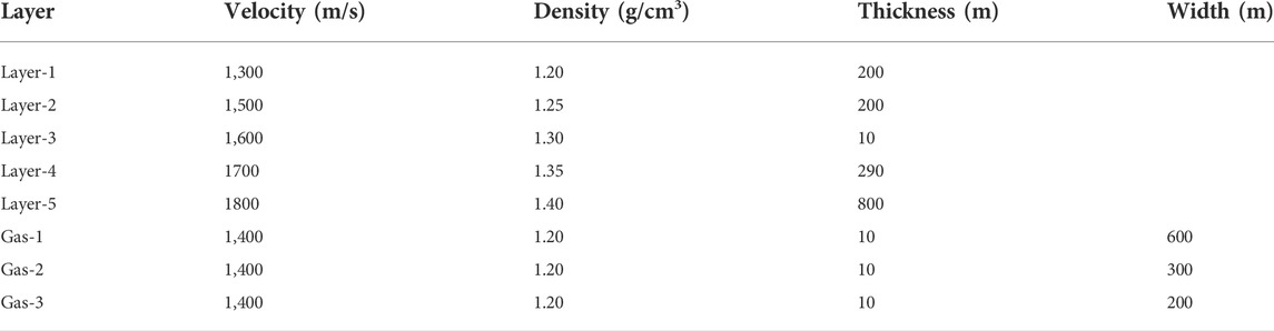
TABLE 1. Geological parameters of the 2-D forward model.

Figures 4C—H represent the single-frequency profile near the target location extracted by applying CWT, CWT—based SST, and improved SST to Figure 4B. They represent the 25 and 35 Hz single-frequency profiles of CWT, CWT—based SST, and improved SST, respectively. The comparison of the three methods shows that the improved SST has the best time–frequency resolution. The three methods can reflect the phenomenon of high-frequency attenuation of gas reservoirs, but the improved SST was more sensitive to frequency changes due to its higher resolution. In particular, the energy group of the gas layer in Figure 4H can hardly be seen in the 35 Hz single-frequency profile, which is sufficient to demonstrate the feasibility of the improved SST method in gas-bearing detection. In addition, it was found that the energy difference between the gas reservoir and surrounding rock in the time spectrum (Figure 4G) was larger than that of the CWT (Figure 4A) and CWT-based SST (Figure 4A), which is helpful for qualitative identification of reservoir boundaries.

3.3 2D unhorizontal layered model

In order to further study the applicability of the improved SST in irregular gas reservoir exploration, we developed a 2D fault model as an example and compared the results to those of the CWT, CWT-based SST, and improved SST methods. This model shown in Figure 5A perceived a gas reservoir at a depth of 300 m. Table 2 displays the specific parameters for each layer. This 2D unhorizontal layer geological model was also forward modeled with a 30 Hz zero-phase Ricker wavelet. Figure 5B displays the pre-stack time migration profile after processing from forward modeling. It is evident that compared with the horizontal layer model, it is more difficult to identify the gas-bearing boundary in the migration profile of the inclined horizon.

FIGURE 5

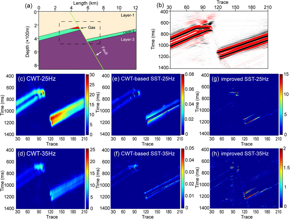
FIGURE 5. Application of the 2-D non-horizontal model and analysis of the instantaneous frequency used the isofrequency section. (A)Forward model, which is created by using the Tesseral 2-D; the black dotted box shows the location of the profile in Panel (B); (B) pre-stack time migration profile of the 2-D forward model in Panel (A). (C) 25 Hz-isofrequency section of the continuous wavelet transform (CWT); (D) 35 Hz-isofrequency section of the CWT; (E) 25 Hz-isofrequency section of the CWT-based SST; (F) 35 Hz-isofrequency section of the CWT-based SST; (G) 25 Hz-isofrequency section of the improved synchrosqueezing transform (SST) in this study; (H) 35 Hz-isofrequency section of the improved SST (these are all plotted with MATLAB, with the “jet” colormap; red indicates higher amplitude).

TABLE 2

TABLE 2. Geological parameters of the fault model.

Figures 5C–H represent the single-frequency profile near the target location extracted by applying CWT (Figures 5C,D), CWT-based SST (Figures 5E,F), and improved SST (Figures 5G,H) methods to Figure 5B. They represent the 25 and 35 Hz single-frequency profiles of CWT, CWT—based SST, and improved SST, respectively. Figure 5 shows that the improved SST can identify the boundary of the reservoir more accurately than the other two methods (Figure 5G). CWT displayed the lowest resolution of the three models. The energy mass of the gas reservoir was not concentrated, and the upper and lower boundaries of the sand body on the right side of fault overlapped. The resolution of the time–frequency distribution of the CWT-based SST was higher than that of CWT, and the sand boundary on both sides of the fault could be identified more accurately. However, it was still difficult to identify the gas reservoir, especially in the 25 single-frequency profiles (Figure 5E).

4 Applications to seismic signals

We used real seismic data from the Tuha basin in Xinjiang as an example to deeply discuss the advantages of the improved SST in gas-bearing reservoir prediction. Due to the influence of many factors, such as attenuation and Earth absorption, in the propagation process of a seismic wave, it showed a high degree of non-stationarity. In the low-frequency profile, shadows appeared beneath the gas reservoir, and the low-frequency shadows gradually disappeared as the frequency increased (Castagna et al., 2003; Chen et al., 2009; Shi et al., 2014). Therefore, we can use these characteristics to detect gas reservoirs. Figure 6 shows a through-well line from 3-D seismic data. The green box indicates a reservoir that has been confirmed to be gas-bearing using drilling data. However, the sand body in the study area changed rapidly in the transverse direction, and a low-frequency, high-amplitude area was present under the gas-bearing layer, namely, a “low-frequency shadow” phenomenon (Ebrom, 2004; Liu 2004; Liu X. et al., 2018). It was difficult to determine the boundary of the sand body with conventional interpretation methods.

FIGURE 6

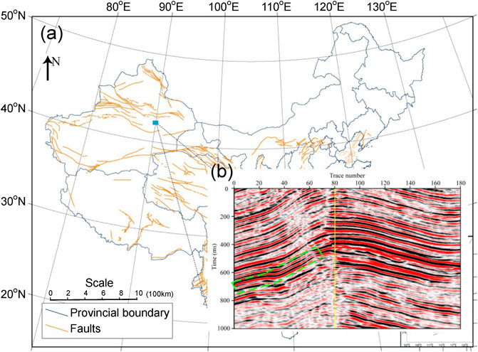
FIGURE 6. Location of the real seismic data. (A) Location of the exploration area where data were collected (blue square). This is created by using the Generic Mapping Tools (GMT) 4, accessed on 1 May 2022; (B) original pre-stack time migration profile of a through-well line from 3-D seismic data; the yellow vertical line represents extracted single-channel seismic data for subsequent analysis; the green box indicates a reservoir by drilling data.

4.1 Single trace

Figure 7A shows the interception of single-channel seismic data of trace No. 80 in Figure 6 and the gas-bearing reservoir near 400 ms. The time spectra of CWT, SST, and improved SST are shown in Figures 7B–D, respectively. It can be seen that compared with CWT, SST had a greater improvement in the adhesion of the energy group, but the vertical time–frequency distribution showed a certain continuity. The improved SST had a higher time–frequency resolution, which could not only improve the problem of energy group diffusion but could also clearly distinguish the gas reservoir from other horizons in the longitudinal direction. The time–frequency characteristics of the wavelet could be accurately determined, especially in the vicinity of the 200–400 ms gas-bearing reservoir. As shown in Figures 7B–D, the dominant frequency for the trace was approximately 30 Hz. Figure 7E shows the comparison between the reconstructed and original seismic data, verifying that the improved synchrosqueezing transform has good reversibility.

FIGURE 7

FIGURE 7. Comparison of single-channel seismic data. (A) Single-channel seismic data for trace No. 80; (B) time–frequency spectra of synthetic seismic trace using the continuous wavelet transform (CWT); (C) time–frequency spectra of synthetic seismic trace using the CWT-based synchrosqueezing transform (SST); (D) time–frequency spectra of synthetic seismic trace using the improved SST; (E) Comparison between the original seismic signal and reconstructed seismic signal by the improved SST. The blue solid line represents the original signal s(t); the red asterisk represents the reconstruction signal [these are all plotted with MATLAB; (B–D) are displayed with the ‘jet’ colormap; red indicates higher amplitude].

4.2 Vertical cross section

Next, we applied the three methods to all traces and computed the time–frequency representation of 30 Hz-signal frequency components to qualitatively identify reservoir boundaries in Figure 8.

FIGURE 8

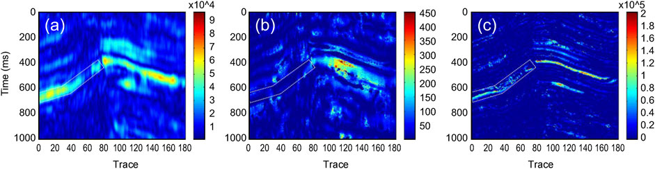
FIGURE 8. 30 Hz-isofrequency profile processed with different approaches. (A) Continuous wavelet transform (CWT); (B) CWT-based synchrosqueezing transform (SST); and (C) improved SST. The white dotted box marks the location of the gas-bearing reservoir (these are all plotted with MATLAB, with the “jet” colormap; red indicates higher amplitude).

It can be seen from Figure 8 that, in general, for the gas reservoirs indicated by the white box, the SST and improved SST had the worst and best time–frequency resolution, respectively. This is because the continuous frequency of the actual data varied greatly, and the original SST could not effectively solve the energy divergence caused by the rapid frequency change, while the improved SST had good adaptability to it. The 20, 30, and 40 Hz single-frequency–time-frequency spectra of the improved synchrosqueezing transform were further extracted and compared (Figure 9). It can be seen that, from 20 to 30 Hz, the time–frequency energy of the reservoir, indicated by the white box, increased with the increasing low-frequency portion. From 30 to 40 Hz, the reservoir time–frequency energy decreased with the increase in high-frequency components. In particular, the boundary range of the isolated gas-bearing reservoir, indicated by the white box, could clearly be determined from the 20–40 Hz variation characteristics.

FIGURE 9

FIGURE 9. Isofrequency profile of data processed by the improved synchrosqueezing transform (SST). (A) 20 Hz-isofrequency profile; (B) 30 Hz-isofrequency profile; and (C) 40 Hz-isofrequency profile. The white dotted box marks the location of the gas-bearing reservoir (these are all plotted with MATLAB, with the “jet” colormap; red indicates higher amplitude).

5 Discussion

In essence, the SST rearranges the energy of each point in the time–frequency spectrum to a position closer to the real time–frequency coordinate of the signal. Specifically, it rearranges the complex spectrum of the WT along the frequency axis. The model test results show that the SST can improve the focusing ability of the original WT and ensure the reversibility of the WT, which has better prospects for application than the time spectrum rearrangement method.

In order to solve the problem that the spectrum energy is not concentrated at a fast frequency change rate in the SST, in this study, we introduced a phase factor before WT using the idea of GFT to improve the SST and enhance its applicability to the frequency change while improving the energy focus. The key to this method was to find $x_0\left(t\right)$ and map the frequency $\omega \left(t\right)$ of the original signal to ${\omega }_0$ by transformation (${\omega }_0$ is here a constant frequency with a rate of change of zero). For a signal $s\left(t\right)$ with a specific expression, if ${\omega }_0$ is given, $x_0\left(t\right)$ can be calculated by the specific expression of $s\left(t\right)$. However, obtaining $x_0\left(t\right)$ is the key problem for the unstable seismic signal $s\left(t\right)$. Olhede and Walden (2005) only used an estimated linear function to obtain $x_0\left(t\right)$ in the improved discrete wavelet packet transform, which was estimated on the time–frequency diagram of the original signal after the discrete wavelet transform. In this study, we used the instantaneous attribute of seismic signal $\omega \left(t\right)$ to obtain $x_0\left(t\right)$ indirectly so as to achieve the purpose of improving the SST. The application results of the model and actual seismic data prove the feasibility of the improved method. On the basis of retaining the inverse transformation, the improved method has high energy focusing ability and applicability to frequency changes.

When the seismic wave propagates in the gas zone, the high-frequency signal attenuates, and the frequency moves toward lower frequencies. At the same time, the low-frequency strong amplitude area will appear below the gas zone, which is often called the “low-frequency shadow” phenomenon (Sheriff, 2002). Taner et al. (1979) identified the low-frequency features under oil and gas reservoirs through complex seismic trace analysis. Castagna et al. (2003) adopted the matching pursuit method to decompose signals in the time–frequency domain and used the anomaly of different instantaneous frequency spectrum energies to directly indicate the existence of oil and gas, that is, the direct hydrocarbon indicator (DHI) technology. Ebrom (2004) studied the correlation between low-frequency shadows and oil and gas storage, and summarized the possible mechanism of low-frequency shadows generated by pre-stack and post-stack seismic data.

Taking Figures 7B–D as an example, the low-frequency shadow phenomenon of the oil and gas reservoir in the target formation was analyzed. As shown in the figure, the location of the reservoir showed a strong energy cluster in both the high frequency and low-frequency bands (dotted line), whereas the low-frequency band below the reservoirs showed a strong energy cluster, which gradually disappeared at the higher band. Due to the insufficient resolution of CWT, the energy group of the reservoir overlapped the low-frequency shadow below (Figure 7B). The CWT-based SST displayed a strong energy distribution in both low- and high-frequency bands (Figure 7C). Compared with the other two methods, the improved synchrosqueezing transform provides high time–frequency resolution to identify the reservoir location more accurately.

Regarding the field data application shown in Figures 8, 9, there was stronger energy distribution in the right part (trace No. 80-160) of the 20-, 30- and 40-isofrequency sections than in the reservoir. Although we have no direct data to confirm whether it is a reservoir or not, based on the geological characteristics of the area and the time–frequency analysis results of this study, we speculate that this part may not be gas-bearing. From the perspective of the geological structure, the gas-bearing layer in the study area is thin, and transverse continuity is poor, while the strong energy mass on the right side is obviously inconsistent with those features. In addition, from the analysis of time–frequency distribution characteristics, as shown in Figure 9, the gas-bearing layer has the weakest energy in the low-frequency band (20 Hz) and strong energy in the high-frequency band (30–40 Hz), while the right strong energy group has strong energy in the 20–30 Hz band and weak energy in the 40 Hz band, which is inconsistent with the time–frequency distribution characteristics of the gas-bearing layer. Combined with the similar phenomenon in the forward model displayed in Figure 5, we speculate that the cause of this phenomenon may be the physical characteristics of the fault itself.

The improved synchrosqueezing transform was applied to the gas reservoir forward model and actual profile; the results showed that the synchrosqueezing transform had higher time-frequency resolution, was more sensitive to the high-frequency attenuation phenomenon, and could describe the gas reservoir distribution range more accurately than the conventional CWT method. It is, therefore, likely to be beneficial for gas detection and the boundary identification of reservoirs in production gas fields.

Data availability statement

The original contributions presented in the study are included in the article/supplementary material; further inquiries can be directed to the corresponding author.

Author contributions

Writing—original draft preparation, CY. Collection of database and the geological interpretation, LC. Methodology, SW. All authors have read and agreed to the published version of the manuscript.

Funding

This research was funded by the National Key Research and Development Program of China (No. 2018YFE0109700) and the Joint Funds of the National Natural Science Foundation of China (No.U2039205).

Acknowledgments

We thank the editors and reviewers for their careful reviews and constructive comments.

Conflict of interest

Author SW was employed by China Electronics Technology Group Corporation.

The remaining authors declare that the research was conducted in the absence of any commercial or financial relationships that could be construed as a potential conflict of interest.

Publisher’s note

All claims expressed in this article are solely those of the authors and do not necessarily represent those of their affiliated organizations, or those of the publisher, the editors, and the reviewers. Any product that may be evaluated in this article, or claim that may be made by its manufacturer, is not guaranteed or endorsed by the publisher.

References

Abry, P., Goncalves, P., and Flandrin, P. (1993). Wavelet-based spectral analysis of 1/f processes. I.E. E.E. Int. Conf. Acoust. 3 (3), 237–240. doi:10.1007/978-1-4612-2544-7_2

CrossRef Full Text | Google Scholar

Auger, F., and Flandrin, P. (1995). Improving the readability of time-frequency and time-scale representations by the reassignment method. IEEE Trans. Signal Process. 43 (5), 10681053–1089587X. doi:10.1109/78.382394

CrossRef Full Text | Google Scholar

Castagna, J. P., Sun, S. J., and Siegfried, R. W. (2003). Instantaneous spectral analysis: Detection of low-frequency shadows associated with hydrocarbons. Lead. Edge 22 (2), 120–127. doi:10.1190/1.1559038

CrossRef Full Text | Google Scholar

Chen, W. C., and Gao, J. H. (2007). Characteristic analysis of seismic attenuation using MBMSW wavelets. Chin. J. Geophys. 50 (3), 722–728. doi:10.1002/cjg2.1086

CrossRef Full Text | Google Scholar

Chen, X. H., He, Z. H., Huang, D. j., and Wen, X. T. (2009). Low frequency shadow detection of gas reservoirs in time-frequency domain. Chin. J. Geophys. 52 (1), 215–221. (in Chinese).

Google Scholar

Daubechies, I., Lu, J. F., and Wu, H. T. (2011). Synchrosqueezed wavelet transforms: An empirical Mode decomposition-like tool. Appl. Comput. Harmon. Anal. 30 (2), 243–261. doi:10.1016/j.acha.2010.08.002

CrossRef Full Text | Google Scholar

Daubechies, I., and Maes, S. (1996). “A nonlinear squeezing of the continuous wavelet transform based on auditory nerve models,” in Wavelets in medicine and biology. Editors A. Aldroubi, and M. Unser (Boca Raton, FL: CRC Press), 527–546.

Google Scholar

Daubechies, I. (2004). Ten lectures on wavelets. Philadelphia: Society for Industrial and Applied Mathematics.

Google Scholar

Daubechies, I., Wang, Y., and Wu, H. T. (2016). ConceFT: Concentration of frequency and time via a multitapered synchrosqueezed transform. Phil. Trans. R. Soc. A 374, 20150193. doi:10.1098/rsta.2015.0193

PubMed Abstract | CrossRef Full Text | Google Scholar

Detka, C. S., and El-Jaroudi, A. (1996). The generalized evolutionary spectrum. IEEE Trans. Signal Process. 44 (11), 2877–2881. doi:10.1109/78.542447

CrossRef Full Text | Google Scholar

Ebrom, D. (2004). The low frequency gas shadow on seismic sections. Lead. Edge 23 (8), 772. doi:10.1190/1.1786898

CrossRef Full Text | Google Scholar

Gao, J. H., Wan, T., Chen, W. C., and Jian, M. (2006). Three parameter wavelet and its applications to seismic data processing. Chin. J. Geophys. 49 (6), 1802–1812. (in Chinese). doi:10.1016/j.apgeochem.2006.08.012

CrossRef Full Text | Google Scholar

Han, J., and Van der Baan, M. (2013). Empirical Mode decomposition for seismic time-frequency analysis. Geophysics 78 (2), 9–19. doi:10.1190/GEO2012-0199.1

CrossRef Full Text | Google Scholar

Han, L. (2013). Research on the methods of high-resolution full spectrum decomposition. Changchun: Jinlin University. [dissertation]. [Changchun, China (in Chinese)].

Google Scholar

Herrera, R. H., Han, J. J., and van der Baan, M. (2014). Applications of the synchrosqueezing transform in seismic time-frequency analysis. Geophysics 79 (3), 55–64. doi:10.1190/geo2013-0204.1

CrossRef Full Text | Google Scholar

Herrera, R. H., Tary, J. B., van der Baan, M., and Eaton, D. W. (2015). Body wave separation in the time-frequency domain. IEEE Geosci. Remote Sens. Lett. 12 (2), 364–368. doi:10.1109/lgrs.2014.2342033

CrossRef Full Text | Google Scholar

Huang, Z., Zhang, J., Zhao, T., and Sun, Y. (2016). Synchrosqueezing S-transform and its application in seismic spectral decomposition. IEEE Trans. Geosci. Remote Sens. 54 (2), 817–825. doi:10.1109/TGRS.2015.2466660

CrossRef Full Text | Google Scholar

Kahoo, A. R., and Siahkoohi, H. R. (2009). “Random noise suppression from seismic data using time-frequency peak filtering,” in Proceedings of the EAGE conference and exhibition (Amsterdam,Netherlands.

Google Scholar

Kodera, K., De Villedary, C., and Gendrin, R. (1976). A new method for the numerical analysis of nonstationary signals. Phys. Earth Planet. Interiors 12 (2–3), 142–150. doi:10.1016/0031-9201(76)90044-3

CrossRef Full Text | Google Scholar

Li, C., and Liang, M. (2012). A generalized synchrosqueezing transform for enhancing signal time-frequency representation. Signal Process. 92 (9), 2264–2274. doi:10.1016/j.sigpro.2012.02.019

CrossRef Full Text | Google Scholar

Li, H. B., Zhao, W. Z., Gao, H., Yao, F. C., and Shao, L. Y. (2004). Characteristics of seismic attenuation of gas reservoirs in wave domain. Chin. J. Geophys. 47 (5), 892–899. doi:10.3321/j.issn:0001-5733.2004.05.022

CrossRef Full Text | Google Scholar

Liu, N., Gao, J., Jiang, X., Zhang, Z., and Wang, P. (2018a). Seismic instantaneous frequency extraction based on the SST-MAW. J. Geophys. Eng. 15 (3), 995–1007. doi:10.1088/1742-2140/aa8cb6

CrossRef Full Text | Google Scholar

Liu, W., Cao, S., Wang, Z., Jiang, K., Zhang, Q., and Chen, Y. (2018b). A novel approach for seismic time-frequency analysis based on high-order syschrosqueezing transform. IEEE Geosci. Remote. Sens. Lett. 99, 1–5. doi:10.1109/LGRS.2018.2829340

CrossRef Full Text | Google Scholar

Liu, X., Liu, H., Xing, L., Yin, Y., and Wang, J. (2018c). Seismic low-frequency shadow beneath gas hydrate in the shenhu area based on the stereoscopic observation system. J. Earth Sci. 29 (3), 669–678. doi:10.1007/s12583-017-0807-8

CrossRef Full Text | Google Scholar

Liu, Y. (2004). Seismic “low frequency shadows” for gas sand reflection. Seg. Tech. Program Expand. Abstr. 23, 1563–1566. doi:10.1190/1.1851138

CrossRef Full Text | Google Scholar

Morlet, J., Arens, G., Fourgeau, E., and Giard, D. (1982b). Wave propagation and sampling theory-Part II: Sampling theory and complex waves. Geophysics 47 (2), 222–236. doi:10.1190/1.1441329

CrossRef Full Text | Google Scholar

Morlet, J., Arens, G., Fourgeau, E., and Glard, D. (1982a). Wave propagation and sampling theory-Part I: Complex signal and scattering in multilayered media. Geophysics 47 (2), 203–221. doi:10.1190/1.1441328

CrossRef Full Text | Google Scholar

Oberlin, T., Meignen, S., and Perrier, V. (20142014). “The Fourier-based synchrosqueezing transform,” in Proceedings on IEEE international conference on acoustics, speech and signal processing (ICASSP) (Florence: Italy), 315–319. doi:10.1109/ICASSP.2014.6853609

CrossRef Full Text | Google Scholar

Odegard, J. E., Baraniuk, R. G., and Oehler, K. L. (1997). “Instantaneous frequency estimation using the reassignment method,” in Proceedings of the SEG meeting 1941–1944 (Dallas, USA.

CrossRef Full Text | Google Scholar

Olhede, S., and Walden, A. T. (2005). A generalized demodulation approach to time-frequency projections for multicomponent signals. Proc. R. Soc. A 461, 2159–2179. doi:10.1098/rspa.2005.1455

CrossRef Full Text | Google Scholar

Pedersen, H. A., Mars, J. I., and Amblard, P. O. (2003). Improving surface-wave group velocity measurements by energy reassignment. Geophysics 68 (2), 677–684. doi:10.1190/1.1567238

CrossRef Full Text | Google Scholar

Potter, R. K., Kopp, G. A., and Green, H. C. (1966). Visible speech. New York: Dover Publications, Inc.

Google Scholar

Potter, R. K., and Steinberg, J. C. (1950). Toward the specification of speech. J. Acoust. Soc. Am. 22 (6), 807–820. doi:10.1121/1.1906694

CrossRef Full Text | Google Scholar

Shang, S. (2014). High-resolution seismic spectral decomposition and its application [dissertation]. Changchun: Jinlin University. [Changchun, China (in Chinese)].

Google Scholar

Sheriff, R. (2002). Encyclopedic dictionary of applied Geophysics. Fourth Edition. Houston: The Society of Exploration Geophysicists.

Google Scholar

Shi, Z. Z., Pang, S., Tang, X. R., and He, Z. H. (2014). Carbonate reservoir characterization based on low-frequency shadow method by matching pursuit algorithm. Lithol. Reserv. 26 (3), 114–118. (in Chinese). doi:10.3969/j.issn.1673-8926.2014.03.019

CrossRef Full Text | Google Scholar

Siahsar, M., Gholtashi, S., Kahoo, A., Marvi, H., and Ahmadifard, A. (2016). Sparse time-frequency representation for seismic noise reduction using low-rank and sparse decomposition. Geophysics 81 (2), 117–124. doi:10.1190/geo2015-0341.1

CrossRef Full Text | Google Scholar

Sinha, S., Routh, P. S., Anno, P. D., and Castagna, J. P. (2005). Spectral decomposition of seismic data with continuous-wavelet transform. Geophysics 70 (6), P19–P25. doi:10.1190/1.2127113

CrossRef Full Text | Google Scholar

Taner, M. T., Koehler, F., and Sheriff, R. E. (1979). Complex seismic trace analysis. Geophysics 44 (6), 1041–1063. doi:10.1190/1.1440994

CrossRef Full Text | Google Scholar

Thakur, G., Brevdo, E., Fučkar, N., and Wu, H. (2013). The Synchrosqueezing algorithm for time-varying spectral analysis: Robustness properties and new paleoclimate applications. Signal Process. 93 (5), 1079–1094. doi:10.1016/j.sigpro.2012.11.029

CrossRef Full Text | Google Scholar

Wang, Q., and Gao, J. (2017). Application of synchrosqueezed wave packet transform in high resolution seismic time-frequency analysis. J. Seismic Explor. 26, 587–599.

Google Scholar

Wang, Q., Gao, J., Liu, N., and Jiang, X. (2018). High-resolution seismic time-frequency analysis using the synchrosqueezing generalized s-transform. IEEE Geosci. Remote Sens. Lett. 15 (3), 374–378. doi:10.1109/LGRS.2017.2789190

CrossRef Full Text | Google Scholar

Wu, G., and Zhou, Y. (2018). Seismic data analysis using synchrosqueezing short time Fourier transform. J. Geophys. Eng. 15 (4), 1663–1672. doi:10.1088/1742-2140/aabf1d

CrossRef Full Text | Google Scholar

Wu, X. Y., and Liu, T. Y. (2009). Spectral decomposition of seismic data with reassigned smoothed pseudo wigner-ville distribution. J. Appl. Geophy. 68 (3), 386–393. doi:10.1016/j.jappgeo.2009.03.004

CrossRef Full Text | Google Scholar

Xue, Y., Cao, J., Wang, X., Li, Y., and Du, J. (2019). Recent developments in local wave decomposition methods for understanding seismic data: Application to seismic interpretation. Surv. Geophys. 40 (5), 1185–1210. doi:10.1007/s10712-019-09568-2

CrossRef Full Text | Google Scholar

Yu, G., Yu, M., and Xu, C. (2017). Synchroextracting transform. IEEE Trans. Ind. Electron. 64, 8042–8054. doi:10.1109/TIE.2017.2696503

CrossRef Full Text | Google Scholar