Indicators of mantle control on the geodynamo from observations and simulations

1 Introduction

Earth’s magnetic field is produced by a dynamo process in the outer core that is driven by convection. This magnetic field engine is enveloped in Earth’s mantle and thus dependent on core-mantle boundary (CMB) conditions. It is well-known from seismological studies that the lowermost mantle is not homogeneous. Large Low Velocity Provinces (LLVPs) are observed below Africa and the Pacific. Although their origin and properties are not fully understood, they are probably warmer than their surroundings and often considered to be denser and chemically distinct [see Garnero et al., 2016, for a review]. They represent large scale thermal heterogeneities that influence the heat flow through the CMB, which forms the top of the geodynamo [see Olson, 2016, for a review]. Estimates of the amplitude of CMB heat flux heterogeneity vary greatly [Mound et al., 2019]. In a review paper, Amit et al. (2015) discussed different methods to infer CMB heat flux from seismic observations and pointed out that non-thermal effects like composition or mineralogical phase changes might play a distinct role in each of the LLVPs and that strong lateral gradients of shear wave velocities are not resolved. More details about the influence of different lower mantle properties on heat flux are discussed by Frost et al.(2022). Existing models of CMB heat flux inferred from seismic observations generally conform to a geometry dominated by spherical harmonic degree and order 2.

The basic interactions between thermal boundary anomalies and rotating convection (Zhang and Gubbins, 1992; 1993; Davies et al., 2009) and dynamos have been elucidated in the presently accessible parameter space. However, the influence of these heterogeneities on the observed magnetic field is still not well understood. Studies from several perspectives and time scales suggest that effects are most likely seen in statistics over long time scales. The observational record relies on both direct measurements and paleomagnetic observations: the first of these provides a high resolution view over decades to a few centuries, a time span that is short with respect to the temporal spectrum the geodynamo, and is in many respects similar to trying to study long term climate using modern weather observations; the latter lack both temporal and spatial resolution, but in principle allow the detection of persistent longer term effects on average field structures and variability.

In reconstructions of the modern field, intense magnetic flux lobes at high latitudes (Bloxham and Gubbins, 1987) and low secular variation in the Pacific region have been interpreted as indications of the mantle’s thermal control on the geodynamo. Regional differences in geomagnetic activity over time scales ranging from observatory records up to millions of years have been discussed for more than 50 years (Doell and Cox, 1971) and linked to inhomogeneities in the lowermost mantle. More recently the striking feature of the present day field known as the South Atlantic Anomaly (SAA), a region over the southern Atlantic and South America where field intensity is notably lower than at comparable latitudes around the rest of the world (Figure 1B) has been studied in a similar context. Paleomagnetic data and global magnetic field reconstructions extending to 100 ka indicate that this might be a recurring feature (Shah et al., 2016; Brown et al., 2018; Trindade et al., 2018; Campuzano et al., 2019; Panovska et al., 2019). There have been suggestions linking a recurring SAA intensity minimum to the long-lived LLVP beneath Africa and associated lateral CMB heat flux variations (Tarduno et al., 2015). The SAA has been drifting westward over the past decades (Mandea et al., 2007; Hartmann and Pacca, 2009), and it is linked to a growing patch of reverse magnetic flux at the CMB [e.g., Gubbins, 1987; Terra-Nova et al., 2017] leading to speculation that it might be the seed location for future reversals (Pavón-Carrasco and De Santis, 2016). This idea remains controversial (Constable and Korte, 2006; Brown et al., 2018; Nilsson et al., 2022) and despite decreases in the field strength over the past few centuries there is no reason to expect that Earth’s magnetic field is in the early stages of a reversal or excursion, in particular as the present dipole moment still seems to lie above the long-term average [see., e.g., Tauxe and Yamazaki, 2015].

FIGURE 1

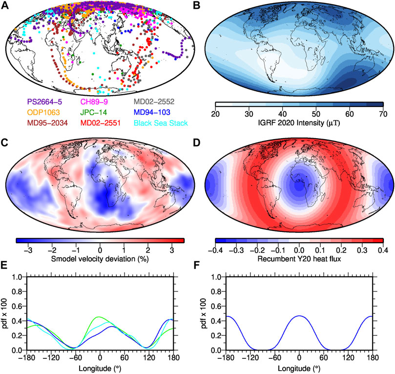
FIGURE 1. (A) Reproduction of VGP paths for the Laschamp excursional paleomagnetic data compiled by Laj and Channell (2015), augmented with the Black Sea record of Nowaczyk et al. (2012). Note that because of ambiguity in setting the average declination PS2664-5 is shifted in longitude relative to the original plot; note further that the central longitude is different in panel (A) than in panels (B–F). (B) Geomagnetic field strength for 2020CE based on IGRF (Alken et al., 2021); (C) Seismic shear wave velocity perturbation at the CMB from model Smodel with blue areas representing LLVPs (see Section 2); (D) Heat flux pattern corresponding to recumbent $Y_2^0$ used for the inhomogeneous CMB condition in the NDS (with continents shown only for ease of comparison). (E) Latitudinally averaged probability density of LLVP areas from seismic model Smodel (green) and below average heat flux regions from models Tlin (blue) and Tp3 (cyan) (see Section 2) as a function of longitude, and (F) the same for below average heat flow from the recumbent $Y_2^0$ pattern (blue).

From the 1990s on a series of models of the time-averaged magnetic field on time scales ranging up to 5 Myr, and covering both normal and reverse polarity intervals, have confirmed the need to include persistent non-axial-dipole and longitudinally varying structure to provide an adequate fit to paleomagnetic observations [see Johnson and McFadden, 2015, for a review]. Several of these models have non-zonal structures [e.g., Cromwell et al., 2018] that resemble attenuated features of the present-day field and could be interpreted as reflecting a long-term signature of CMB heat flux patterns. Attenuation is to be expected as a result of the time-averaging reducing variability due to flux patch mobility, due to limited spatial sampling, and the complete lack of intensity data used to derive these models (intensities are needed for resolution at high latitudes). More pronounced signatures of high latitude flux lobes are seen in the shorter term averages of time-varying field models spanning 10–100 ky that routinely make use of both directional and intensity data (see maps of B_r at the CMB in Figures 2E–H). Their positions and overall strength vary across the different time intervals averaged and presumably also reflect variable temporal and spatial resolution for each model.

FIGURE 2

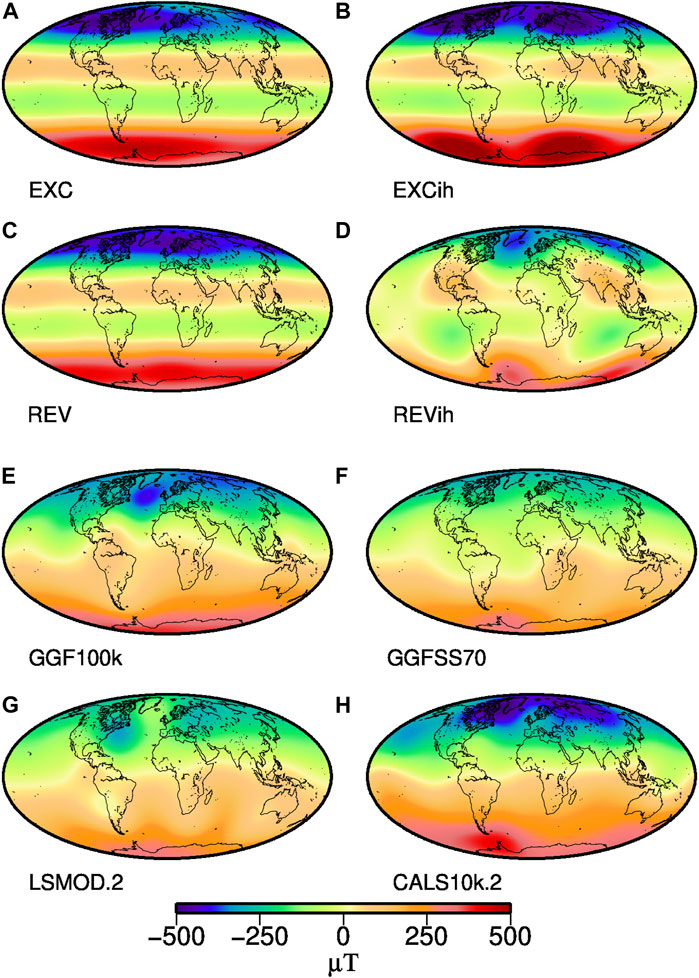
FIGURE 2. Time-averaged radial magnetic field at the CMB up to SH degree and order 5 (with continents shown for reference) from the four NDSs ((A,C) with homogeneous boundary conditions, and (B,D) are inhomogeneous) and the four PFMs (E–H) studied in this work. See Section 3 for details on the models. In order to avoid cancelling of positive and negative flux over times of opposing polarity the sign of the radial field was reversed whenever the axial dipole had reverse polarity for these averages.

There is also ongoing controversy about whether the extreme geomagnetic field changes found during reversals and excursions have characteristic geometries that might be indicative of mantle control on the geodynamo. Reversals and excursions are often considered to reflect the same kind of underlying process with both being driven by decay and recovery of the axial dipole field contribution to the field [e.g., Valet and Plenier, 2008; Amit et al., 2010; Wicht and Meduri, 2016; Korte et al., 2019]. Each features strong directional field changes and weak field intensities, but they are distinguished by reversals including a lasting polarity switch while excursions exhibit varying degrees of globally or regionally observed reversed field directions following which the field returns to its previous polarity. There are indications that excursions generally take less time than a full reversal and Gubbins (1999) has proposed that this reflects that an excursion may fail to propagate reverse flux into the inner core, though this interpretation has been questioned by Wicht (2002). The full mechanics of reversals and excursions and their relation are still not understood but excursions can probably be seen as aborted reversals (Cox et al., 1975; Valet et al., 2008), and may appear regionally or globally depending on how weak the axial dipole contribution gets in comparison to the non-dipole field (Brown and Korte, 2016; Panovska et al., 2019).

Following traditional paleomagnetic analyses, virtual geomagnetic poles (VGPs) and their changes with time have been widely used to investigate excursions and reversals from individual paleomagnetic records. VGPs [e.g., Merrill et al., 1996] remove the large geographic variation in directions attributable to dipole fields. The comparison of VGPs and VGP paths during excursions and reversals from different locations thus provide some indications about the global field dipolarity or more general field geometry, although this is not always easy to interpret. Several paleomagnetic studies of reversals and excursions reported VGPs paths falling preferentially in American and East Asian longitudes [e.g., Tric et al., 1991; Laj et al., 1991; Clement, 1991; Love, 1998; Hoffman, 2000]. It was first noted by Laj et al., 1991 that preferred VGP longitudes from these records lie in regions of high seismic p-wave velocity in the lowermost mantle. Later, Laj et al. (2006) and Laj and Channell (2015) reported preferred VGP paths, that are similar for two prominent excursions but in somewhat different longitudinal bands than the previous results drawn mainly from reversals. The reproduction of their results for the Laschamp excursion in Figure 1A demonstrates similar VGP paths from several locations, that actually seem to fall in LLVP regions (compare with blue regions in Figure 1C - taking note of the different central longitude in a). Figure 1A also indicates that other records may show quite different VGP paths, and indeed other studies have been used to suggest that the longitudinal VGP distributions are indistinguishable from random [e.g., Prévot and Camps, 1993]. It has also been argued that systematic data biases may generate artificial structures: uneven spatial sampling leads to VGP longitudes preferentially located 90^◦ away from site locations (Egbert, 1992; Valet et al., 1992); or longitudinal confinement of VGPs might arise from smoothing across non-antipodal stable directions before and after a geomagnetic reversal, due to remanence acquisition processes in sediments [e.g., Langereis et al., 1992].

Based on Figures 1A,B open questions from the observations are thus whether we can identify robust links between mantle thermal structure and 1) longitudinal concentrations of low latitude VGPs, 2) what is the relationship of any longitudinal concentrations of VGPs to the flux lobes and/or that mantle thermal structure, and 3) are there recurrent regions of low field strength similar to the SAA in low to mid-latitude regions that may be linked to heterogeneous thermal boundary conditions?

A different perspective is provided by investigating the potential influence of heterogeneous CMB heat flow in numerical dynamo simulations (NDS). This has been implemented either by imposing a heterogeneous heat flux pattern linked to seismic observations or a simple spherical harmonic degree 2 proxy that resembles large scale features of the seismic models [see, e.g., Christensen and Wicht, 2015, for a review]. Coe et al. (2000), Christensen and Olson (2003) and Kutzner and Christensen (2004) investigated VGP paths from simulations with imposed heat flow heterogeneities and find some longitudinal preference of VGP paths over regions of high heat flux. They inferred that VGPs might tend to cluster in the regions of increased heat flux which cause magnetic flux concentrations due to strong up- and downwelling of core fluid (Christensen and Wicht, 2015).

A new generation of global spherical harmonic Paleomagnetic Field Models (PFMs) that span up to 100 kyr and include several magnetic field excursions offers the opportunity to study the distribution of an extended suite of geomagnetic field properties globally. Korte et al., ([2019) and Panovska et al., ([2019) have already noted that VGP paths predicted from these models exhibit preferred longitudes. Statistical comparisons to Numerical Dynamo Simulations are now possible as the same analyses can be applied to both. The NDS are particularly useful for testing the quantitative robustness of observations that seem to link longitudinal variations in specific field properties to variations in core-mantle boundary (CMB) conditions: in the real world these are inferred from the positions of LLVPs (Figure 1C), while for the NDS we use the simplified “recumbent $Y_2^0$” geometry (Dziewonski et al., 2010) shown in Figure 1D, a combination of the conventionally used $Y_2^2$, $Y_2^0$ and $Y_1^1$ spherical harmonic functions, that roughly resembles the seismic structure of the lower mantle and may represent the stable part of the D″ thermal heterogeneity (Dziewonski et al., 2010). Maps of the time-averaged radial magnetic field at the CMB are given in Figures 2A–D and already confirm that the time-averaged longitudinal structure in the form of high latitude flux lobes along with other features is quite pronounced in NDS with inhomogeneous boundary conditions, and also visible in the four PFMs in panels E–H.

In what follows we first outline estimates of CMB heat flux variations based on seismic tomographic models and indicate how they relate to the simplified geometry used in two of the four examples of NDS (Section 2) that we use for comparison to our PFM results. In Section 3 we describe the numerical simulations and paleofield models that we use and introduce the magnetic field properties analyzed on regular grids from them in Section 4. We use the NDS products in Section 5.1 to test links between heat flux and concentrations of low latitude VGPs and intensity minima, respectively, predicted under both dense temporal and spatial sampling and under restricted conditions equivalent to the paleomagnetic data distributions used to build PFMs. In Section 5.2 we analyze four recently developed PFMs, reconstructions of the paleomagnetic field for past millennia up to an age of 100 ka, to investigate the distribution of intensity minima and VGP paths globally. The findings from the analyses on NDSs and PFMs are discussed and compared in Section 6. We conclude with a brief synthesis of our findings.

2 Proxies for core-mantle boundary structure

Direct observation of the heat flux at the CMB is not possible, but lateral heterogeneities in seismic velocity structure near the CMB are mapped using the methods of global seismic tomography [e.g., Masters et al., 2000; Hernlund and McNamara, 2015], and these are commonly thought to reflect and have been translated into estimates of heat flow variations under a number of simplifying assumptions [e.g., Amit et al., 2015]. The past 4 decades have seen the development of multiple seismic tomography models using a range of different techniques and various kinds of seismic data. As with geomagnetic models, global models of seismic velocities and CMB heat flow depend on the underlying data and, in particular in the latter case, several assumptions [e.g., Becker and Boschi, 2002; Amit et al., 2015]. For our study, we aim to identify features that can be considered robust across all models and find an average global seismic shear wave model that can be used as a proxy input to determine variation in heat flow across the CMB.

Hosseini et al., (2018) have compiled over 30 seismic tomography models in an easy-to-use web-based tool called SubMachine. They noticed a good general agreement of LLVP locations among most models, so that averages can be used to produce a representative S-velocity anomaly. The proxy of LLVPs used here is derived from S10mean, itself an average of 10 tomography models (Doubrovine et al., 2016), plus 3 more (SP12RTS-S (Koelemeijer et al., 2016), SEISGLOB2 (Durand et al., 2017) and TX2019slab-S (Lu et al., 2019)), and we call it Smodel in the following (shown in Figure 1C). Before computing the average, the amplitudes are normalized by SubMachine. All these seismic models are evaluated at 2,889 km depth, equivalent to the CMB depth used in geomagnetic field models. Values that fall below the average are considered to define the LLVPs, values above as associated with seismically faster regions.

Shear wave velocity variations may be translated into lateral variability in CMB heat flux, and this is again an uncertain process, in which it is difficult to take appropriate account of variations in properties distinct from thermal effects. We considered two distinct models which (together with the LLVP distributions discussed above) are used to assess correlations with PFM results in Section 5.2. The heat flux distributions are based on the mantle tomography model of Masters et al.(2000) and were derived by Amit and Choblet (2009), the first as a linear transformation into the thermal boundary condition (referred to as model Tlin in the following), the other, non-linear transformation, additionally takes account of the post-Perovskite phase transitions in the lowermost mantle (model Tp3). As with the seismic models, we use all values above and below the mean, respectively, to define areas of high or low CMB heat flux from these models.

Figure 1E depicts probability density functions of the seismic LLVP values (green) or below average heat flux values from the two models Tlin (blue) and Tp3 (cyan) integrated over the latitudes to provide a function of longitude. The differences between the lines gives an indication about the uncertainties in these proxies, and we will use all three in the following as they peak at different longitudes. Figure 1F illustrates the probability density function in longitude of the “LLVPs” represented by the recumbent $Y_2^0$ structure shown in panel D.

3 Numerical dynamo simulations and paleomagnetic field models

3.1 Numerical dynamo simulations

We used four long numerical simulations runs, two with and two without outer boundary heat flow heterogeneity and varying levels of occurrences of transitional and reversing field. The simulations, originally reported in Sprain et al. (2019) were obtained by solving the Boussinesq dynamo equations in rotating spherical shell geometry with constant material properties. The dimensionless variables that characterise the solution are the Ekman number E=5 × 10^–4, the ratio of viscous to Coriolis effects, the Prandtl number Pr=1, the ratio of viscous to thermal diffusivity, the magnetic Prandtl number Pm of 5 or 10 (see individual models below), the ratio of viscous to magnetic diffusion, and the Rayleigh number Ra, measuring the strength of the driving buoyancy distribution. The choice of parameters is motivated by the necessity for long simulations with reversals and excursions, which necessitates relatively high Ekman number. The magnetic Prandtl number was set to ensure dynamo action and then Ra was varied until reversals arose. We note that for a systemtic study of NDS, two pairs of models with the same buoyancy conditions and Ra values and one with homogeneous and one with heterogeneous boundary conditions in each pair should be used. However, for comparison purposes to PFM results it is no disadvantage to have four somewhat arbitrary and different NDS that show behaviour that has been found in other NDS before. All our simulations use no-slip and electrically insulating conditions on both boundaries, and the ratio of inner to outer boundary radii is 0.35.

The spherical harmonic coefficients of the magnetic fields of these models initially are dimensionless and defined at Earth’s surface. Absolute values or magnitudes are not relevant for this study, but for easier intuitive comparison we normalised the time-averaged axial dipole coefficient to the average value of the GGF100 k field model (see Section 3.2) and scaled all other coefficients by the same factor. The models come in time steps with varying overall length. We are not considering event durations or frequencies in this study, therefore we did not scale the time steps to calendar years. For easier handling (to have mostly 4 digit times) we start the time step count for each of the models at 1,000 as shown in Figure 3. This figure illustrates several features of the models by dipole moment, dipole tilt (latitude of dipole axis), axial $(g_1^0)$ and equatorial ($g_1^1$, $h_1^1$) spherical harmonic dipole coefficients, and power in dipole (D) and large-scale (SH degrees 2 to 5) non-dipole (ND) coefficients. For each model the average radial magnetic fields at the outer boundary over all time steps are shown in Figures 2A–D, where we can see that the inhomogeneous boundary conditions (panels B and D) give rise to systematic non-zonal structure. In contrast the homogeneous boundary conditions in panels A and C are quite uniform in longitude. Note that the longitudinal orientation is completely arbitrary in the homogeneous case and only defined for agreement of the imposed heat flux structure with the LLVPs in the heterogeneous case. Continents and longitudes are used only as reference frame for ease of discussion here.

FIGURE 3

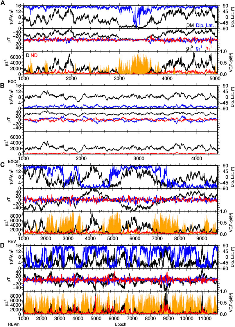
FIGURE 3. Some characteristics of the four numerical dynamo simulations EXC (A), EXCih (B), REV (C) and REVih (D). Top panels contain dipole moment (DM, black, left axis) and dipole latitude (blue, right axis), middle panels contain the three dipole coefficients $g_1^0$ (black), $g_1^1$ (blue) and $h_1^1$ (red), bottom panels contain dipole (black) and large-scale non-dipole (red, SH degrees 2–5) power at Earth’s surface. Orange histograms (right axis) give the fraction of VGPs falling between 45^◦N and 45^◦S from an equal area grid of 1666 VGP positions.

3.1.1 Models with homogeneous outer boundary heat flux

Two of the numerical models have homogeneous outer boundary conditions. One of them, called model EXC in the following (with Pm=10, fixed codensity flux on both boundaries, Ra=350, duration of 6.7 magnetic diffusion times), has only one clear excursion at time steps around 3,500, although some transitional VGPs are found at a few other times (Figure 3A). Note that transitional VGPs do not only occur when the dipole tilt is strong, but more generally when dipole power is very low. The other model, called REV here (with Pm=5, fixed codensity on the inner boundary and fixed codensity gradient on the outer boundary, Ra=450, duration of 5.1 magnetic diffusion times), has multiple reversals (Figure 3C) with relatively few stable intervals of strong dipole dominance. It spans nearly double the time of model EXC.

3.1.2 Models with heterogeneous outer boundary heat flux

The other two models have the recumbent spherical harmonic $Y_2^0$ heat flow pattern imposed at the outer boundary (see Figure 1D), with a normalized amplitude of 1.5. We orient them such that the simulated “LLVPs”, i.e., below average heat flux areas, agree in longitude with the seismic LLVPs and show continents on the simulations in all figures for ease of comparison. The model named EXCih here (with Pm=10, fixed codensity flux on both boundaries with recumbent $Y_2^0$ pattern, Ra=100, duration of 5.24 magnetic diffusion times) was expected to have at least one excursion or some transitional data, but is in fact strongly dipole dominated and fully stable over the entire time interval (Figure 3B). Model REVih (with Pm=5, fixed codensity flux on both boundaries with recumbent $Y_2^0$ pattern, Ra=150, duration of 13.87 magnetic diffusion times), in contrast, has very few stable intervals. It reverses frequently for irregular intervals and has transitional VGPs most of the time (Figure 3D). The power in the dipole and non-dipole terms have similar levels at Earth’s surface much of the time, and axial and equatorial dipole contributions often are of the same order in this model.

3.2 Global spherical harmonic paleomagnetic models

We include four paleomagnetic global field reconstructions in our analysis. All of them are based on spherical harmonics in space and cubic B-splines in time. Spatial and temporal resolution are determined by regularizations, that trade off a good fit to the data against smoothness of the model, in order to minimize the influence of data distribution and uncertainties, in particular with regard to overly complicated artificial field structures [for details see, e.g., Korte et al., 2009]. The spherical harmonic models show power comparable to the present day in the spatial power spectrum up to degrees four to five for all four models, suggesting this level of spatial resolution in regions where data are available. The temporal resolution varies notably as discussed below. Figure 4 illustrates the same quantities for the PFMs as Figure 3 for the NDSs, and once again the average radial magnetic fields at the CMB over all time steps are shown in Figures 2E–H.

• GGF100k (Panovska et al., 2018) is the longest currently available model, spanning the past 100 kyrs based on more than one hundred sediment records and the available volcanic (and for the recent past archeomagnetic) data (Figure 4A). Due to the varying quality and resolution of the sediment records the temporal resolution of this model is notably lower than of the other three. It covers many millennia of stable field as well as several reported excursions, namely the Post-Blake (∼95 ka), the Norwegian-Greenland Sea (∼65 ka), the Laschamps (∼41 ka), the Mono Lake/Auckland (∼30–34 ka), an event around 28 ka, and the Hilina Pali excursion (∼17 ka). Not all of them are clearly seen in the model, partly due to the limited model resolution. Given the dispute about the age/identity of the excursion recorded at the Mono Lake location [see Marcaida et al., 2019] we use the double name Mono Lake/Auckland for the event around ∼30–34 ka, following a suggestion by Laj et al., (2014).

• GGFSS70 (Panovska et al., 2021) is based on just nine selected high resolution records with high-quality age models and as good as possible global coverage. It spans the interval 70–15 ka (Figure 4B), and particularly the Norwegian-Greenland Sea and Laschamps excursions appear well represented by this model of notably higher temporal resolution than GGF100k.

• LSMOD.2 (Korte et al., 2019) spans the interval 50–30 ka around the Laschamps and Mono Lake/Auckland excursions with similar temporal resolution as GGFSS70 (Figure 4C). It is based on 12 sediment records. Some of them are stacks where all contributing data have been carefully assessed for regional consistency. All age scales have been updated with the latest available information. Compared to the others this model has only a few short intervals of stable field polarity.

• CALS10k.2 (Constable et al., 2016) spans the past 10 kyrs based on 74 sediment records, volcanic and archeomagnetic data. This time interval is stably dipole dominated and does not include any field excursion. However, the model has been used to simulate the potential excursion mechanism of a decaying and recovering axial dipole with smaller scale secular variation proceeding as during stable polarity (Brown and Korte, 2016), i.e. all coefficients except for the axial dipole remained unchanged. Here, we use the original CALS10k.2 for intensity investigations and include the toy model with the axial dipole coefficient linearly scaled to decay to zero and recover over the full duration of the model, as depicted in Figure 4C in our VGP analysis.

FIGURE 4

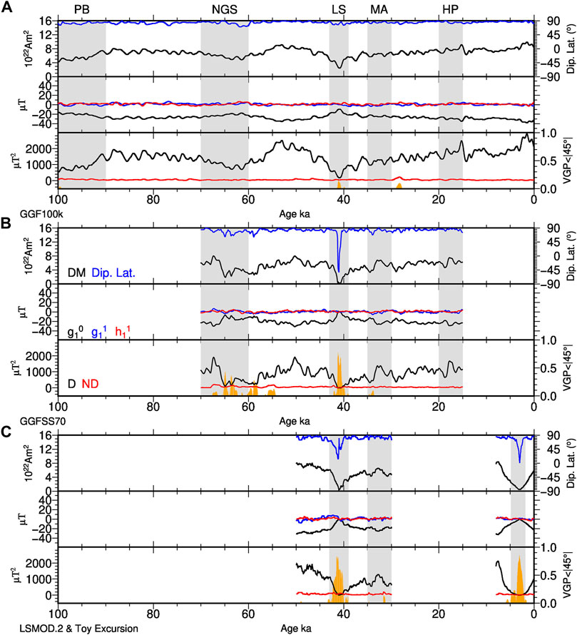
FIGURE 4. Some characteristics of the four paleomagnetic field reconstructions GGF100k (A), GGFSS70 (B), LSMOD.2 and the artificial excursion created in a toy model from CALS10k.2 (C). Top panels contain dipole moment (DM, black, left axis) and dipole latitude (blue, right axis), middle panels contain the three dipole coefficients $g_1^0$ (black), $g_1^1$ (blue) and $h_1^1$ (red), bottom panels contain dipole (black) and non-dipole (red, SH degrees 2–5) power at Earth’s surface. Gray areas indicate times of reported field excursions: Post-Blake (PB, ∼100–90 ka), Norwegian-Greenland Sea (NGS, ∼70–60 ka), Laschamps (LS, ∼42–40 ka), Mono Lake/Auckland (MA, ∼35–30 ka) and Hilina Pali (HP, ∼20–15 ka), and the artificial excursion in the toy model (∼1–5 ka). Orange histograms (right axis) in the bottom panels give the fraction of VGPs falling between 45^◦N and 45^◦S from an equal area grid of 1666 VGP positions.

Times for which field excursions have been reported in the literature are shaded, and mostly are reflected by dipole lows in all the models. The fractions of transitional VGPs between 45^◦N and 45^◦S are also shown as a function of time (see Section 4.2) in orange and in general high numbers coincide with known excursions. Note the reduced numbers of transitional VGPs in GGF100k compared to GGFSS70 due to the lower temporal resolution. Enhanced non-dipole power around 28 ka and 55 ka causes some further transitional VGPs in models GGF100k and GGFSS70, respectively. The Mono Lake/Auckland excursion is not so clearly seen even in the high resolution models, and dipole lows and a few transitional VGPs are found around 34 and 31 ka, suggesting that this might be a series of regional events during a time of low dipole strength. Similarly, GGFSS70 suggests that the Norwegian-Greenland Sea excursion might be more than one event.

4 Methods: Analyses of field properties

We use distributions of two different field quantities across the records to assess their capacity and robustness for affirming the previously known sensitivity of NDS results to thermal structure and identifying links to LLVP and heat flux maps in PFMs.

4.1 Intensity minima

First, we consider minimum field intensity at Earth’s surface represented across the entire time frame for each model. In the modern field this is associated with the SAA (Figure 1B). Given the large-scale structure of the field at nearly 3,000 km distance from the source we simply determine the location of the absolute global intensity minimum (Fmin) for each time step and study the geographic distribution of these values in the form of global probability density distributions (pdf) that are normalized to be comparable for different overall numbers of data (We later checked and found that using the lowest 1–10% of intensity results in smoother distributions but otherwise does not change our results.) We choose number and density of time steps depending on the duration and temporal resolution of the individual PFM and NDS models. Only relative variations within the distributions are of interest. Next we assess the longitudinal distributions of intensity minima by summing the number of occurrences over all latitudes and normalizing to provide pdfs as a function of longitude. For creating the pdfs we choose the kernel width as 15^◦, to underline the long-wavelenth trends from the temporally averaged PFMs. This is done for easier visual comparison and to account for the comparatively sparse sampling compared to the much longer time series from the NDSs, for which the pdfs with narrower and wider kernels differ much less. We look for correlations between the distributions in minimum intensity in NDS or PFM and our CMB heat flow proxies, i.e., the predictions from the recumbent $Y_2^0$ structure or Smodel, Tlin and Tp3, respectively.

4.2 Virtual geomagnetic poles

VGPs lying in latitudes between 45^◦N and S are commonly interpreted as indications of transitional magnetic field behaviour corresponding to either excursions or reversals. We calculate VGP paths over the full time intervals of all models on an equal area global grid of locations at 1,666 points and locate all transitional VGPs. As for the intensity minima, we study their distributions through global and longitudinal pdfs and compare them to the CMB heat flow proxies. Note that the requirement for sampling transitional VGPs will produce smaller numbers of samples than in the minimum intensity distributions, since not every time slice has transitional VGPs.

4.3 Robustness tests

We applied a test with synthetic data to check for effects of the uneven spatial data distribution available for constructing the PFMs on the robustness of detection of preferred longitudes. As the models mostly rely on sediment records that provide time series over the duration of the model, either with not too dissimilar temporal resolution (CALS10k.2, LSMOD.2, GGFSS70) or taking into account differences in temporal smoothing (GGF100k), we only consider the spatial distribution here. We selected 1,200 time steps from the REV (model REVpart) and REVih (model REVihpart) simulations, respectively, that reflect the different Fmin and transitional VGP distributions of these models (see Section 5.1) to predict data at the 12 locations with records used for the LSMOD.2 field reconstruction. We sample the NDS to construct synthetic data sets and apply the methods that were used for the paleomagnetic reconstructions and present the results in the next Section. It should be noted that differences in the time spans covered by the various models may also impact the results if long records are needed to recover the full longitudinal distributions of either low latitude VGPs or intensity minima.

5 Results

5.1 Numerical dynamo simulations

We begin with results of our analysis on the four complete NDSs described in Section 3.1, before conducting robustness tests on spatial distributions.

5.1.1 Numerical dynamo simulation intensity minima

Figure 5 comprises four panels from the four NDS, showing global and longitudinal pdf of minimum intensities computed over the whole time span of each model, respectively. The latitudinal distributions are rather well balanced between N and S hemisphere in all numerical simulations. For all models that have excursions or reversals the intensity minima span all latitudes (Figures 5A,C,D). Not surprisingly, the minima are more strongly confined to equatorial latitudes the more dipole dominated a simulation is (Figures 5A,B). The homogeneous outer boundary numerical simulations (Figures 5A,C) exhibit fairly uniform distributions in longitude, with no strongly preferred regions, although EXC does seems to have a slight preference for Indian Ocean/Western Pacific compared to Eastern Pacific/Atlantic longitudes (but remember that this is an arbitrary orientation). This deviation from a uniform distribution probably is a consequence of the finite simulation time. Inhomogeneous outer boundary simulations, on the other hand, show very clear preferred longitudinal bands for F minima, about equally strong with widths ranging from about 40^◦ to 140^◦E and W (Figures 5B,D). A clear visual correlation is seen between the distribution of F minima and the recumbent $Y_2^0$ heat flow structure imposed in these simulations. Areas of preferred minimum intensity are those of above average heat flux. This result is the same both for the strongly dipole dominated EXCih, where global minima never occur in mid to high latitudes, and REVih, the least dipole dominated of our NDS. Despite the significant amount of time that this simulation spends in transitional field stage (see frequent occurrence of transitional VGPs in Figure 3D) the minima are still concentrated in equatorial latitudes, as also noted by Terra-Nova et al., (2019).

FIGURE 5

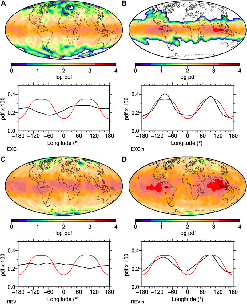
FIGURE 5. Distributions of intensity minima in four different numerical dynamo simulations, with continents shown for ease of comparison to PFM results. The top panels give their global density distribution, the bottom panels the longitudinal density distribution (black line) in comparison to the distribution of above average CMB heat flux or “non-LLVP” areas (red) from a recumbent $Y_2^0$ structure. Simulations EXC (A) and REV (C) have homogeneous heat flow, while EXCih (B) and REVih (D) have the recumbent $Y_2^0$ heat flow imposed. EXC (A) and EXCih (B) are more strongly dipole-dominated than REV (C) and REVih (D). Global minima never occur in the white areas in panel b, due to the strong dipole dominance of that simulation.

5.1.2 Numerical dynamo simulation - virtual geomagnetic poles

Figure 6 shows the distributions of VGPs falling between 45^◦N and S for the three NDS that have them. Note that there are hardly any time intervals without transitional VGPs, because the simulations are less dipole dominated than the PMFs, in particular in REV and REVih (see Figures 3A,C,D). The longitudinal distribution of REVih is clearly bimodal and in rough agreement with the imposed outer boundary heat flux (Figure 6C), although the actual VGP longitude peaks are displaced westward by some tens of degrees.

FIGURE 6

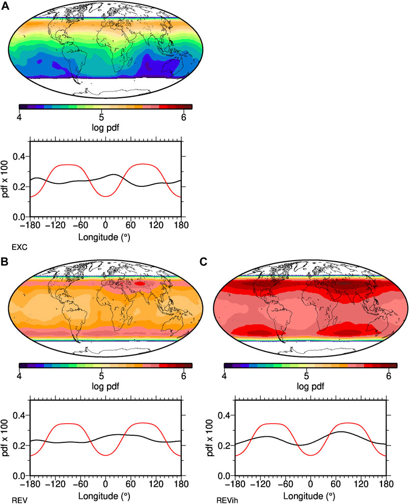
FIGURE 6. Distribution of all transitional VGPs falling between 45^◦N and 45^◦S from a regular grid of VGP paths in three numerical geodynamo simulations. The top panels give their global density distribution, the bottom panels have longitudinal density profiles (black line), in comparison to the distribution of above average CMB heat flux (red) from the recumbent $Y_2^0$ structure imposed on the simulations. EXC (A) only has one excursions, and also REV (B) is more strongly dipole dominated than REVih (C). Simulations EXC (A) and REV (C) have homogeneous CMB heat flow, while REVih (C) has inhomogeneous CMB heat flow imposed.

The pdfs of both model REV and EXC (including only one excursion) are closer to uniform, although each exhibits structure that might be interpreted as two slight maxima. For REV a very broad one is centered around 50^◦E and a narrow one around 180^◦E (Figure 6B). Model EXC, including only one excursion, reflects two narrow, somewhat similar preferred VGP longitudes more clearly, around 20^◦E and 180^◦E (Figure 6A). Neither correlates with the areas of above average heat flux imposed on REVih, and we should not expect this given that EXC and REV have homogeneous heat flow. In fact a slight negative correlation is observed and this must reflect the fact that the average fields in Figure 2 do have some residual non-zonal structure despite the time-averaging and this may be reflected in the transitional samples.

Smaller dynamic range in the peak-to-peak amplitudes for EXC and REV pdfs than for REVih point to support for preferred VGP paths in REVih, the NDS with inhomogeneous boundary conditions, but the paths are not fully aligned with the heat flux maxima.

The effects of time-averaging, i.e., impact of short sample length, can be investigated by an analysis of individual transitional events from the long NDS model runs and this sheds light on the difference in distributions between EXC, REV and REVih. As the few examples in Figure 7 demonstrate, individual excursions or reversals drawn from both REV and REVih give somewhat different transitional VGP distributions that do not necessarily reflect what is obtained from a longer record. They often appear roughly bi-modal, probably reflecting the dominance of non-zonal quadrupole field structure when the dipole contribution is weak, but the peak longitudes vary among events. This is particularly obvious in the case of heterogeneous CMB conditions (Figure 7B), where only a large number of events provides a sufficient statistical sample to reflect the CMB structure in transitional VGP distribution.

FIGURE 7

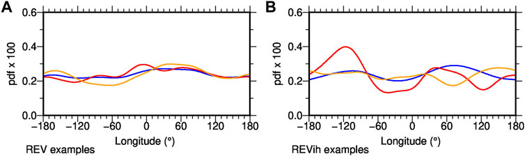
FIGURE 7. Transitional VGP distributions from long runs of numerical simulations that include multiple transitional events (blue lines) compared to distributions obtained from two examples of individual events from the same models (red, orange). (A) Examples from homogeneous model REV and (B) from inhomogeneous model REVih.

5.1.3 Synthetic data and spatial distribution tests

The influence of uneven spatial distribution in the paleomagnetic data-based reconstructions is assessed in Figure 8 using the 1,200 time sample records described in Section 4.3. Panels a and b show minimum F pdfs from complete spatial sampling (black) and reconstructed from the incompletely spatially sampled (dashed line) models over longitude for model REVpart without and model REVihpart with outer boundary heterogeneities. Panels C and D show the same for transitional VGPs. Light gray lines reproduce the distributions for the entire record as in Figures 5, 6, panels C and D.

FIGURE 8

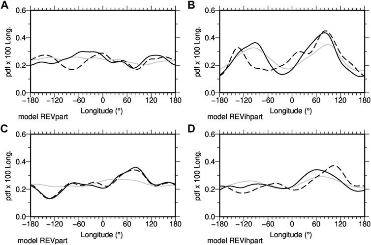
FIGURE 8. Longitudinal distributions of intensity minima (A,B) and of transitional VGPs (C,D) in numerical simulations with homogeneous (model REVpart, panels (A,C)) and inhomogeneous outer boundary conditions (model REVihpart, panels (B,D)). The solid lines are from the shorter intervals of the original models as used for this test, with the dashed lines from their reconstructions, respectively. The gray lines are the distributions from the full length simulations as in Figures 5, 6, panels (C,D). The reconstructions are from synthetic data obtained from the short intervals of the original models at the locations where real data are available.

For the homogeneous model REVpart, the small departures from uniformity in the minimum intensity distribution (gray) are accentuated by the short temporal sample (black) and altered by the uneven data distribution (dashed). Once again the dynamic range in the distribution is larger for model REVihpart and slightly enhanced in the short record, while the uneven data distribution modifies the longitudinal peaks. In both cases, the data distribution mainly influences the western hemisphere, where the peak longitudes are clearly shifted in the reconstructions. It seems likely that combined influences from data distribution and structure of the CMB inhomogeneity give rise to these differences.

In the homogeneous case of VGP distributions (panel C) the short temporal sample accentuates the departures from uniformity adding significantly more structure to the distribution, but the diminished spatial sampling has relatively little additional impact. The dynamic range in both REVpart (C) and REVihpart (D) VGP distributions is similar, but the peak positions for REVihpart with its inhomogeneous CMB conditions are less stable under the available spatial sampling.

Another consideration is whether there is any influence from setting declination to zero mean over the time interval of paleomagnetic reconstructions to compensate for the fact that real data sediment records are in general azimuthally unoriented. We found that the mean declination of the synthetic records is in general within ±15^◦. Small deviations in this range occur in both NDS models, and are not just specific to model REVihpart with the heterogeneous outer boundary conditions. We conclude that the distributions observed in the NDSs are not influenced by persistent declination deviation from zero mean in certain locations.

5.2 Paleomagnetic field models

5.2.1 Paleomagnetic field model intensity minima

Figure 9 shows the pdfs of minimum intensity from the four PFMs over their respective full time spans. As these intervals are mostly shorter than the NDSs, in particular comprising much fewer transitional events than simulations REV and REVih, the F minima are generally more confined to equatorial and mid latitudes. The maps suggest that the latitudinal distributions are slightly biased towards the southern hemisphere as might be expected from the hemispherical asymmetry found in model CALS10k.2 as described by Constable et al. (2016). All four models show preferred longitudinal bands, with some similarities, but also significant differences which might be attributable to differences in temporal and spatial coverage of the underlying data. All four models have peaks around $\sim 75^{◦}$W, broad and centered somewhat further east in GGF100k, and peaking slightly further west in CALS10k.2. These longitudes are slightly west of the center of the present-day SAA (see also Terra-Nova et al. (2019), Figure 5), probably reflecting the observed recurrence of a similar structure on long timescales in the longer models. More F minima are also often found further west, peaking around 120^◦W in GGFSS70 and 135^◦W in LSMOD.2. In the eastern hemisphere, all models except for GGF100k often have F minima around 130–140^◦E and, with variable numbers, between ∼0 and 60^◦E. All models suggest that intensity minima rarely fall in the region 60 to 120^◦E, around 180^◦E, and except for GGF100k they also have relatively small numbers between 0 and 60^◦W.

FIGURE 9

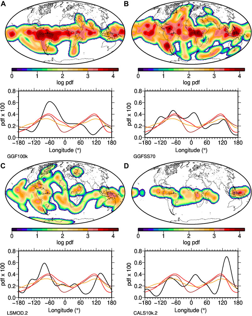
FIGURE 9. Distribution of intensity minima in four data-based paleomagnetic field reconstructions. The top panels give their global density distribution, the bottom panels longitudinal density distribution (black) in comparison to distributions of above average CMB heat flux (models Tlin in red, Tp3 in orange) and non LLVP areas from model Smodel (brown). GGF100k (A) spans 0–100 ka with relatively low temporal resolution, GGFSS70 (B) spans 20–70 ka, LSMOD.2 (C) spans 20–50 ka and CALS10k.2 (D) spans approximately the past 10 ka. See text for details.

Comparing these distributions to three proxies of CMB heterogeneity does not give a clear direct correlation with any of their generally bimodal structures. However, all reconstructions except for the shortest CALS10k.2/Toy model have higher concentrations of F minima in the non-LLVP or presumed above average heat flux area in the western hemisphere, and drops with some resemblance particularly to the distribution of seismic LLVPs (brown Smodel curve) towards the zero meridian. All except for the lowest resolution GGF100k have a high density of F minima around the eastern edge of the eastern non-LLVP area, although much of those longitudes are otherwise characterised by rare occurrences of F minima in most of the models.

The real situation clearly is more complicated than the NDS case. Several factors may play a role: the statistics are less robust due to the shorter time intervals; although both LSMOD.2 and GGFS70 have good temporal resolution they are based on limited spatial data distributions (12 and 9 records respectively); CALS10k.2/toy is the shortest of all and only covers 10 ky, which could lead to the kind of mismatches seen in Figures 8A,B. GGF100k has good spatial coverage, and the longest record of all which is clearly important but poor chronological constraints in some of the underlying records may have contributed to a lack of resolution in spatial structure. Differences in the distributions (Figure 9) probably reflect some of the differences in the time-averaged CMB field structures in Figure 2.

5.2.2 Paleomagnetic field model - virtual geomagnetic poles

Comparing the transitional VGP distributions (Figure 10) from the PFMs it is obvious that the GGF100k is most distinctive. Despite the fact that this model covers the largest number of excursions, the transitional VGPs are regionally confined and do not cover the full latitudinal range between 45^◦N and S. This certainly reflects the model’s low temporal resolution, and a distortion of the longitudinal pdf by incomplete sampling of excursional events seems very possible. The locus of the peak in VGP distribution over North America lies to the west of that for the intensity distribution that corresponds to low values in the time-average B_r at mid to high southern latitudes. In contrast to the results from the other three models there is no apparent alignment of the GGF100k VGP distribution with LLVP signals.

FIGURE 10

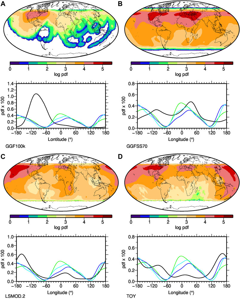
FIGURE 10. Distribution of all transitional VGPs falling between 45^◦N and S from a regular grid of VGP paths in three data-based paleomagnetic field reconstructions and a toy model simulating a possible excursion mechanism. The top panels give their global density distribution, the bottom panels the longitudinal density distribution (black), in comparison to the distribution of below average CMB heat flux (models Tlin in blue, Tp3 in cyan) and LLVP areas from model Smodel (green). GGF100k (A) spans 0–100 ka with relatively low temporal resolution, GGFSS70 (B) spans 20–70 ka, LSMOD.2 (C) spans 20–50 ka and the toy model (D) is based on CALS10k.2 spanning approximately the past 10 ka with an artificial excursion simulated by the axial dipole decaying to zero and recovering over this time interval. Transitional VGPs are never found in white areas.

The distributions of GGFSS70, LSMOD.2 and even the toy excursion model all have a peak in European longitudes, slightly east of the zero meridian and aligned well with one of the LLVPs, and in particular with the heat flux proxy determined by linear transformation (Tlin, blue line). The three models all have a bimodal distribution, although with varying amplitudes. In LSMOD.2, the second peak in the Pacific region agrees well with the other LLVP. In the toy model there is a rough agreement with the LLVP, but with a secondary peak over the Americas further east, and the peak over the Americas also appears in GGFSS70, but in this case without an enhanced number of transitional VGPs in the Pacific directly in the LLVP region. However, in general transitional VGPs are found less often in the North Atlantic/South American and Asian regions in all models, roughly agreeing with the regions outside the LLVPs or of enhanced CMB heat flux. Overall we find that the distributions of the three higher resolution models broadly agree with transitional VGPs preferentially falling in the LLVP, or presumed below average CMB heat flux areas. This (visually) good correlation is surprising given the low number of events and the diverse results found in individual events in NDSs. One reason to view these VGP results with some skepticism is that, confusingly, the correlations in these VGP distributions appears to be opposite to the results from the NDSs where the peaks are more closely linked to above average heterogeneous boundary heat flow rather than below average in the PFMs.

6 Discussion

Summarizing our findings, the complete NDSs do reflect whether core boundary heat flow is homogeneous or not both in global distribution of intensity minima and transitional VGPs. In agreement with earlier results (Coe et al., 2000; Kutzner and Christensen, 2004), the VGP distributions peak at longitudes of high boundary heat flow, i.e. outside the “LLVPs”, where convection likely is stronger than in low heat flux areas and flux concentrations occur from both up- and downwelling (Kutzner and Christensen, 2004). The signature from the VGPs is much less pronounced than for the intensity minima which peak at similar longitudes in NDS examples. Robustness tests with short records and limited data distributions suggest that the VGP record may be difficult to interpret in the studied PFMs.

Figures 2A–D, showed time averages of the radial magnetic field at the outer core boundary from the four NDSs, which do not have simple dipolar structure. In each case the models have reverse flux patches or bands present at low to mid latitudes in both northern and southern hemispheres with the distribution nearly zonal in simulations EXC and REV. In EXCih and REVih, there are concentrations of high normal flux in high latitudes, and more diffuse reverse flux patches in low latitudes. The reverse flux patches lie in the longitudinal ranges of high heat flow as imposed by the recumbent $Y_2^0$ proxy, and lead to the preferred occurrence of intensity minima at Earth’s surface in these regions. However, we note that Terra-Nova et al. (2019) found a parameter-dependent shift of surface intensity minima in other NDS, and more generally shifts between heat flux and resulting magnetic field in NDS have been previously discussed and are not yet understood (Aubert et al., 2007; Takahashi et al., 2008). The high-latitude normal flux in REVih does not correspond with the longitudinal distribution of transitional VGPs, the flux patches are displaced eastward beneath North Atlantic and Kamchatka longitudes, while the VGP concentrations are below North America and Central Asian longitudes and their southern hemisphere counterparts (Figure 6). This reflects a complicated relation between radial field structure and VGPs that is hard to unravel in the absence of better equatorial sampling of the VGPs. Earlier results reviewed by Christensen and Wicht (2015) noted that the VGPs tend to point to regions of magnetic flux concentration like those seen in equatorial regions for the modern field, which form in regions of high heat flux due to strong up- and down-welling. The average distributions plotted here are unable to resolve that question.

The results for the PFMs are less clear, and similarly, the time-averaged radial magnetic field patterns at the CMB (Figures 2E,F) are less clearly linked to the lower mantle structures. In the western hemisphere, normal flux concentrations at high latitudes again tend to lie to east of the peaks in transitional VGP distributions for all models. Inconsistencies and complexities across the models in the central and eastern hemispheres make it difficult to unravel a clear overall signature for the VGPs, especially given that the only apparent alignments are opposite to those found for the NDS.

The low intensity signature in the PFMs is more easily understood in terms of average field structure as in each case it can be linked to low or even reverse B_r flux in Figures 2E–H. In the western hemisphere weak (if not always reversed) flux at low latitudes are found near the high heat flux longitudes between the LLVPs (Figure 1D), in general agreement with our finding of peaks in intensity minima distribution around these longitudes. The PFM intensity minima distribution results were less conclusive for the eastern hemisphere, where the CMB radial field maps also differ more, and only one of the models, GGFSS70, has indications of weak magnetic flux throughout the Indian Ocean. CALS10k.2, LSMOD.2 and GGF100k have indications for normal flux concentrations at high latitudes near the high heat flux longitudinal band, which would only have limited influence on the low latitude intensity distribution, though. While it seems conceivable that CMB properties in the eastern higher seismic velocity area could be different from the western one, any such interpretation should be carefully considered in light of an assessment the paleomagnetic data distribution: LSMOD.2 and GGFSS70 clearly have less data in Asian longitudes than in the western hemisphere. Our experiments on the NDS with short time samples, and limited spatial data distribution helped to highlight some potential pitfalls in analyzing the PFMs, and a potential unfortunate combination of too short records, sparse data coverage, and less reliable data can adversely influence our ability to detect existing correlations. We also note that using only the lowest intensity values might bias the results if two (or more) minima related to mantle influence were always present, but this does not seem to be a problem as we do find a symmetric bimodal distribution for the NDS where such a simple pattern was imposed.

The results of our comparisons of the transitional VGP distributions to heat flux proxies do not help to decide between the possible interpretations. We found a surprisingly good correlation with CMB heat flux given the small number of events, but it is the opposite of what is expected from the NDS results. This is hard to understand and might be a coincidence from sampling too few events–the results of GGFSS70 and LSMOD.2 will be dominated by the properties Laschamps excursion (see numbers of transitional VGPs in Figure 4), and Figure 7B gives an example where an individual event (orange line) from an NDS has nearly inverse correlation to the distribution obtained from a large number of events. The comparison of Figures 2, 10 suggests that transitional VGP concentrations occur well away from strong CMB magnetic flux concentrations in time averages of the models (e.g., GGF100k over North America; LSMOD.2 over the Pacific and Europe), while the flux distribution might be different during the transitional times.

7 Conclusion

We have investigated the spatial distributions of global magnetic field intensity minima and of transitional VGPs from four global paleomagnetic field reconstructions and four numerical dynamo simulations regarding indications of influences of CMB heat flux heterogeneities linked to lowermost mantle structures. The PFMs cover 10–100 kyr and include up to five reported excursions, but the Laschamps excursion dominates the results. We also included an empirically simulated excursion based on the 10 kyr CALS10k.2 model. The spherical harmonic PFMs allow a broader investigation than those traditionally based on VGP paths from individual locations, and give access to global distributions of several observed field properties. Two of the NDSs have homogeneous heat flow through the CMB, the other two have a recumbent $Y_2^0$ heat flow pattern imposed, that reflects very roughly the geometry of the seismologically observed LLVPs in the lower mantle. In each case, one of the NDSs is dipole dominated and has only one or no excursion, and the other has a large number of excursions and reversals, but few intervals of clear dipole dominance.

The analyses of the NDSs reflect previously reported correlations between preferred VGP paths and above average heat flux (that is non-LLVP) areas at the CMB as a statistical average when a large number of events are studied. However, the preferred VGP longitudes do not align directly with high latitude flux concentrations found in the average radial field at the CMB. We note that individual events often display two (slightly) preferred bands for transitional VGPs at different longitudes in simulations both with and without heterogeneous CMB structure. The use of short records produces less robust results (Figure 7), and limited spatial data distributions, that likely interact with the inhomogeneous structure, are likely to further limit detailed interpretations of the PFM records (Figure 8).

With this in mind, we should not expect similar correlations from the PFMs, which include only a small number of excursions and no reversals. With one exception the PFMs, including a toy model where an excursion has been simulated by enforcing decay and recovery of the axial dipole while keeping the rest of secular variation as during the past 10 kyr do have bi-modal longitudinal distributions of transitional VGPs that appear correlated with LLVPs, a result that is incompatible with results from the numerical simulations. We infer that in the PFMs the lack of sufficient sampling of transitional VGPs inhibits robust results for the longitudinal distributions of VGPs.

In contrast, the preferred locations of minimum field intensity are clearly correlated with above average heat flux patterns at the outer boundary in the simulations. In the paleomagnetic reconstructions, this seems to be the case for the western, but not the eastern hemisphere. Although this might be interpreted to reflect differences in LLVP structures in east versus west, this cannot be distinguished from inadequacies in the PFMs. Using a test with synthetic data we cannot rule out that the models are simply less reliable in the eastern hemisphere. We tentatively suggest that the minimum intensity distribution in the western hemisphere supports influence from CMB heat flux on the geodynamo. However, this may not be detectable based on the rather short time span covered and incomplete sampling of dynamo behavior in the PFMs. Further work and better temporal and spatial data coverage are required to decide if the absence of correlation in the eastern hemisphere is due to PFM limitations or differences about the relation between seismic observations and CMB heat flux properties in the eastern compared to the western hemisphere.

Data availability statement

Publicly available datasets were analyzed in this study. This data can be found here: The paleomagnetic field models are available in the EarthRef.org digital archive at https://earthref.org/ERDA/2207/(CALS10k.2), https://earthref.org/ERDA/2472/ (GGFSS70), https://earthref.org/ERDA/2382/ (GGF100k), and from the GFZ Data Services as \citep{korte19d} https://dataservices.gfz-potsdam.de/panmetaworks/showshort.php?id=escidoc:3763902 The seismic tomography models were obtained from https://www.earth.ox.ac.uk/∼smachine/cgi/index.php.

Author contributions

MK originally designed the study with improvements to analyses and presentation of results from discussions with all co-authors. MK carried out the analyses with contributions from CC. The first version of the manuscript was written by MK, and subsequently revised with contributions from all co-authors.

Funding

MK acknowledges alumni support from the Alexander von Humboldt foundation for a research stay with CC that initiated this study. CD gratefully acknowledges funding from the NERC Pushing the Frontiers grant ref NE/V010867/1. He and CC are moreover jointly funded by NERC and NSF under grants ref NE/V009052/1. SP and NSF EAR 1953778 which supported this work. SP gratefully acknowledges the Discovery Fellowship at the GFZ Potsdam, Germany. Supported within the funding programme Open Access Publikationskosten“ Deutsche Forschungsgemeinschaft (DFG, German Research Foundation) - Project Number 491075472.

Acknowledgments

We thank Hagay Amit for providing grids of the three heat flux models. All plots were created with the Generic Mapping Tools, https://www.generic-mapping-tools.org/ (Wessel et al., 2019). We thank two reviewers whose comments helped to clarify and improve aspects of the paper.

Conflict of interest

The authors declare that the research was conducted in the absence of any commercial or financial relationships that could be construed as a potential conflict of interest.

Publisher’s note

All claims expressed in this article are solely those of the authors and do not necessarily represent those of their affiliated organizations, or those of the publisher, the editors and the reviewers. Any product that may be evaluated in this article, or claim that may be made by its manufacturer, is not guaranteed or endorsed by the publisher.

References

Alken, P., Thébault, E., Beggan, C., Amit, H., Aubert, J., Baerenzung, J., et al. (2021). International geomagnetic reference field: The thirteenth generation. Earth Planets Space 73, 49. doi:10.1186/s40623–020–01288–x

CrossRef Full Text | Google Scholar

Amit, H., and Choblet, G. (2009). Mantle-driven geodynamo features—Effects of post-perovskite phase transition. Earth Planets Space 61, 1255–1268. doi:10.1186/bf03352978

CrossRef Full Text | Google Scholar

Amit, H., Choblet, G., Olson, P., Monteux, J., Deschamps, F., Langlais, B., et al. (2015). Towards more realistic core-mantle boundary heat flux patterns: A source of diversity in planetary dynamos. Prog. Earth Planet. Sci. 2, 26. doi:10.1186/s40645-015-0056-3

CrossRef Full Text | Google Scholar

Amit, H., Leonhardt, R., and Wicht, J. (2010). Polarity reversals from paleomagnetic observations and numerical dynamo simulations. Space Sci. Rev. 155, 293–335. doi:10.1007/s11214-010-9695-2

CrossRef Full Text | Google Scholar

Aubert, J., Amit, H., and Hulot, G. (2007). Detecting thermal boundary control in surface flows from numerical dynamos. Phys. Earth Planet. Interiors 160, 143–156. doi:10.1016/j.pepi.2006.11.003

CrossRef Full Text | Google Scholar

Becker, T. W., and Boschi, L. (2002). A comparison of tomographic and geodynamic mantle models. Geochem. Geophys. Geosystems 3. doi:10.1029/2000gc000168

CrossRef Full Text | Google Scholar

Bloxham, J., and Gubbins, D. (1987). Thermal core–mantle interactions. Nature 325, 511–513. doi:10.1038/325511a0

CrossRef Full Text | Google Scholar

Brown, M. C., and Korte, M. (2016). A simple model for geomagnetic field excursions and inferences for palaeomagnetic observations. Phys. Earth Planet. Interiors 254, 1–11. doi:10.1016/j.pepi.2016.03.003

CrossRef Full Text | Google Scholar

Brown, M., Korte, M., Holme, R., and Gunnarson, S. (2018). Earth’s magnetic field is probably not reversing. Proc. Natl. Acad. Sci. U. S. A. 115, 5111–5116. doi:10.1073/pnas.1722110115

PubMed Abstract | CrossRef Full Text | Google Scholar

Campuzano, S. A., Gómez-Paccard, M., Pavón-Carrasco, F. J., and Osete, M. L. (2019). Emergence and evolution of the south atlantic anomaly revealed by the new paleomagnetic reconstruction shawq2k. Earth Planet. Sci. Lett. 512, 17–26. doi:10.1016/j.epsl.2019.01.050

CrossRef Full Text | Google Scholar

Christensen, U. R., and Olson, P. (2003). Secular variation in numerical geodynamo models with lateral variations of boundary heat flow. Phys. Earth Planet. Interiors 138, 39–54. doi:10.1016/s0031-9201(03)00064-5

CrossRef Full Text | Google Scholar

Christensen, U. R., and Wicht, J. (2015). “Numerical dynamo simulations,” in Treatise on geophysics. Editor G. Schubert. 2nd ed. (Amsterdam, Netherlands: Elsevier), Vol. 8, 245–277.

CrossRef Full Text | Google Scholar

Clement, B. M. (1991). Geographical distribution of transitional VGPs: Evidence for non-zonal equatorial symmetry during the matuyama-brunhes geomagnetic reversal. Earth Planet. Sci. Lett. 104, 48–58. doi:10.1016/0012-821x(91)90236-b

CrossRef Full Text | Google Scholar

Coe, R. S., Hongre, L., and Glatzmaier, G. A. (2000). An examination of simulated geomagnetic reversals from a palaeomagnetic perspective. Philosophical Trans. R. Soc. Lond. Ser. A Math. Phys. Eng. Sci. 358, 1141–1170. doi:10.1098/rsta.2000.0578

CrossRef Full Text | Google Scholar

Constable, C., and Korte, M. (2006). Is Earth’s magnetic field reversing. Earth Planet. Sci. Lett. 246, 1–16. doi:10.1016/j.epsl.2006.03.038

CrossRef Full Text | Google Scholar

Constable, C., Korte, M., and Panovska, S. (2016). Persistent high paleosecular variation activity in southern hemisphere for at least 10 000 years. Earth Planet. Sci. Lett. 453, 78–86. doi:10.1016/j.epsl.2016.08.015

CrossRef Full Text | Google Scholar

Cox, A., Hillhouse, J., and Fuller, M. (1975). Paleomagnetic records of polarity transitions, excursions, and secular variation. Rev. Geophys. 13, 185–189. doi:10.1029/rg013i003p00185

CrossRef Full Text | Google Scholar

Cromwell, G., Johnson, C. L., Tauxe, L., Constable, C. G., and Jarboe, N. A. (2018). PSV10: A global data set for 0–10 ma time-averaged field and paleosecular variation studies. Geochem. Geophys. Geosyst. 19, 1533–1558. doi:10.1002/2017gc007318

CrossRef Full Text | Google Scholar

Davies, C. J., Gubbins, D., and Jimack, P. K. (2009). Convection in a rapidly rotating spherical shell with an imposed laterally varying thermal boundary condition. J. Fluid Mech. 641, 335–358. doi:10.1017/s0022112009991583

CrossRef Full Text | Google Scholar

[Dataset] Korte, M., and Brown, M. (2019). Lsmod.2 - global paleomagnetic field model for 50–30 ka bp. Potsdam: GFZ Data Services.

Google Scholar

Doell, R. R., and Cox, A. (1971). Pacific geomagnetic secular variation. Science 171, 248–254. doi:10.1126/science.171.3968.248

PubMed Abstract | CrossRef Full Text | Google Scholar

Doubrovine, P. V., Steinberger, B., and Torsvik, T. H. (2016). A failure to reject: Testing the correlation between large igneous provinces and deep mantle structures with edf statistics. Geochem. Geophys. Geosyst. 17, 1130–1163. doi:10.1002/2015gc006044

CrossRef Full Text | Google Scholar

Durand, S., Debayle, E., Ricard, Y., Zaroli, C., and Lambotte, S. (2017). Confirmation of a change in the global shear velocity pattern at around 1000 km depth. Geophys. J. Int. 211, 1628–1639. doi:10.1093/gji/ggx405

CrossRef Full Text | Google Scholar

Dziewonski, A. M., Lekic, V., and Romanowicz, B. A. (2010). Mantle anchor structure: An argument for bottom up tectonics. Earth Planet. Sci. Lett. 299, 69–79. doi:10.1016/j.epsl.2010.08.013

CrossRef Full Text | Google Scholar

Egbert, G. D. (1992). Sampling bias in vgp longitudes. Geophys. Res. Lett. 19, 2353–2356. doi:10.1029/92gl02549

CrossRef Full Text | Google Scholar

Frost, D. A., Avery, M. S., Buffett, B. A., Chidester, B. A., Deng, J., Dorfman, S. M., et al. (2022). Multidisciplinary constraints on the thermal-chemical boundary between Earth’s core and mantle. Geochem. Geophys. Geosyst. 23, e2021GC009764. doi:10.1029/2021gc009764

CrossRef Full Text | Google Scholar

Garnero, E. J., McNamara, A. K., and Shim, S.-H. (2016). Continent-sized anomalous zones with low seismic velocity at the base of Earth’s mantle. Nat. Geosci. 9, 481–489. doi:10.1038/ngeo2733

CrossRef Full Text | Google Scholar

Gubbins, D. (1987). Mechanism for geomagnetic polarity reversals. Nature 326, 167–169. doi:10.1038/326167a0

CrossRef Full Text | Google Scholar

Gubbins, D. (1999). The distinction between geomagnetic excursions and reversals. Geophys. J. Int. 137, F1–F4. doi:10.1046/j.1365-246x.1999.00810.x

CrossRef Full Text | Google Scholar

Hartmann, G. A., and Pacca, I. G. (2009). Time evolution of the south atlantic magnetic anomaly. An. Acad. Bras. Cienc. 81, 243–255. doi:10.1590/s0001-37652009000200010

CrossRef Full Text | Google Scholar

Hernlund, J. W., and McNamara, A. K. (2015). “The core-mantle boundary region,” in Treatise on geophysics. Editor G. Schubert. 2nd ed. (Amsterdam, Netherlands: Elsevier), Vol. 7, 461–519.

CrossRef Full Text | Google Scholar

Hoffman, K. A. (2000). Temporal aspects of the last reversal of Earth’s magnetic field. Philosophical Trans. R. Soc. Lond. Ser. A Math. Phys. Eng. Sci. 358, 1181–1190. doi:10.1098/rsta.2000.0580

CrossRef Full Text | Google Scholar

Hosseini, K., Matthews, K. J., Sigloch, K., Shephard, G. E., Domeier, M., and Tsekhmistrenko, M. (2018). Submachine: Web-based tools for exploring seismic tomography and other models of Earth’s deep interior. Geochem. Geophys. Geosyst. 19, 1464–1483. doi:10.1029/2018gc007431

PubMed Abstract | CrossRef Full Text | Google Scholar

Johnson, C. L., and McFadden, P. (2015). “The time-averaged field and paleosecular variation,” in Treatise on geophysics. Editor G. Schubert. 2nd ed. (Amsterdam, Netherlands: Elsevier), Vol. 5, 385–417.

CrossRef Full Text | Google Scholar

Koelemeijer, P., Ritsema, J., Deuss, A., and Van Heijst, H.-J. (2016). Sp12rts: A degree-12 model of shear-and compressional-wave velocity for Earth’s mantle. Geophys. J. Int. 204, 1024–1039. doi:10.1093/gji/ggv481

CrossRef Full Text | Google Scholar

Korte, M., Brown, M. C., Panovska, S., and Wardinski, I. (2019). Robust characteristics of the Laschamp and Mono Lake geomagnetic excursions: Results from global field models. Front. Earth Sci. 7. doi:10.3389/feart.2019.00086

CrossRef Full Text | Google Scholar

Korte, M., Donadini, F., and Constable, C. (2009). Geomagnetic field for 0-3ka: 2. A new series of time-varying global models. Geochem. Geophys. Geosyst. 10, Q06008. doi:10.1029/2008GC002297

CrossRef Full Text | Google Scholar

Kutzner, C., and Christensen, U. R. (2004). Simulated geomagnetic reversals and preferred virtual geomagnetic pole paths. Geophys. J. Int. 157, 1105–1118. doi:10.1111/j.1365-246x.2004.02309.x

CrossRef Full Text | Google Scholar

Laj, C., and Channell, J. E. T. (2015). “Geomagnetic excursions,” in Treatise on geophysics. Editor G. Schubert. 2nd ed. (Amsterdam, Netherlands: Elsevier), Vol. 5, 343–363.

CrossRef Full Text | Google Scholar

Laj, C., Guillou, H., and Kissel, C. (2014). Dynamics of the Earth magnetic field in the 10–75 kyr period comprising the Laschamp and Mono Lake excursions: New results from the French Chaîne des Puys in a global perspective. Earth Planet. Sci. Lett. 387, 184–197. doi:10.1016/j.epsl.2013.11.031

CrossRef Full Text | Google Scholar

Laj, C., Kissel, C., and Roberts, A. P. (2006). Geomagnetic field behaviour during the Iceland basin and Laschamp geomagnetic excursions: A simple transitional field geometry? Geochem. Geophys. Geosyst. 7, Q03004. doi:10.1029/2005GC001122

CrossRef Full Text | Google Scholar

Laj, C., Mazaud, A., Weeks, R., Fuller, M., and Herrero-Bervera, E. (1991). Geomagnetic reversal paths. Nature 351, 111–112. doi:10.1038/359111b0

CrossRef Full Text | Google Scholar

Langereis, C., Van Hoof, A., and Rochette, P. (1992). Longitudinal confinement of geomagnetic reversal paths as a possible sedimentary artefact. Nature 358, 226–230. doi:10.1038/358226a0

CrossRef Full Text | Google Scholar

Love, J. (1998). Paleomagnetic volcanic data and geometric regularity of reversals and excursions. J. Geophys. Res. 103, 12435–12452. doi:10.1029/97jb03745

CrossRef Full Text | Google Scholar

Lu, C., Grand, S. P., Lai, H., and Garnero, E. J. (2019). Tx2019slab: A new p and s tomography model incorporating subducting slabs. J. Geophys. Res. Solid Earth 124, 11549–11567. doi:10.1029/2019jb017448

CrossRef Full Text | Google Scholar

Mandea, M., Korte, M., Mozzoni, D., and Kotzé, P. (2007). The magnetic field changing over the southern african continent: A unique behaviour. South Afr. J. Geol. 110, 193–202. doi:10.2113/gssajg.110.2-3.193

CrossRef Full Text | Google Scholar

Marcaida, M., Vazquez, J. A., Stelten, M. E., and Miller, J. S. (2019). Constraining the early eruptive history of the mono craters rhyolites, California, based on 238u-230th isochron dating of their explosive and effusive products. Geochem. Geophys. Geosyst. 20, 1539–1556. doi:10.1029/2018gc008052

CrossRef Full Text | Google Scholar

Masters, G., Laske, G., Bolton, H., and Dziewonski, A. (2000). The relative behavior of shear velocity, bulk sound speed, and compressional velocity in the mantle: Implications for chemical and thermal structure. Earth’s deep interior Mineral Phys. Tomogr. atomic Glob. scale 117, 63–87. doi:10.1029/GM117p0063

CrossRef Full Text | Google Scholar

Merrill, R. T., McElhinny, M. W., and McFadden, P. L. (1996). The magnetic field of the Earth. Cambridge, MA: Academic Press.

Google Scholar

Mound, J., Davies, C., Rost, S., and Aurnou, J. (2019). Regional stratification at the top of Earth’s core due to core–mantle boundary heat flux variations. Nat. Geosci. 12, 575–580. doi:10.1038/s41561-019-0381-z

CrossRef Full Text | Google Scholar

Nilsson, A., Suttie, N., Stoner, J. S., and Muscheler, R. (2022). Recurrent ancient geomagnetic field anomalies shed light on future evolution of the south atlantic anomaly. Proc. Natl. Acad. Sci. U. S. A. 119, e2200749119. doi:10.1073/pnas.2200749119

PubMed Abstract | CrossRef Full Text | Google Scholar

Nowaczyk, N. R., Arz, H. W., Frank, U., Kind, J., and Plessen, B. (2012). Dynamics of the Laschamp geomagnetic excursion from Black Sea sediments. Earth Planet. Sci. Lett. 351-352, 54–69. doi:10.1016/j.epsl.2012.06.050

CrossRef Full Text | Google Scholar

Olson, P. (2016). Mantle control of the geodynamo: Consequences of top-down regulation. Geochem. Geophys. Geosyst. 17, 1935–1956. doi:10.1002/2016gc006334

CrossRef Full Text | Google Scholar

Panovska, S., Constable, C. G., and Korte, M. (2018). Extending global continuous geomagnetic field reconstructions on timescales beyond human civilization. Geochem. Geophys. Geosyst. 19, 4757–4772. doi:10.1029/2018GC007966

CrossRef Full Text | Google Scholar

Panovska, S., Korte, M., and Constable, C. G. (2019). One hundred thousand years of geomagnetic field evolution. Rev. Geophys. 57, 1289–1337. doi:10.1029/2019rg000656

CrossRef Full Text | Google Scholar

Panovska, S., Liu, J., Korte, M., and Nowaczyk, N. (2021). Global evolution and dynamics of the geomagnetic field in the 15–70 kyr period based on selected paleomagnetic sediment records. JGR. Solid Earth 126, e2021JB022681. doi:10.1029/2021jb022681

CrossRef Full Text | Google Scholar

Pavón-Carrasco, F. J., and De Santis, A. (2016). The South Atlantic Anomaly: The key for a possible geomagnetic reversal. Front. Earth Sci. 4, 40. doi:10.3389/feart.2016.00040

CrossRef Full Text | Google Scholar

Prévot, M., and Camps, P. (1993). Absence of preferred longitude sectors for poles from volcanic records of geomagnetic reversals. Nature 366, 53–57. doi:10.1038/366053a0

CrossRef Full Text | Google Scholar

Shah, J., Koppers, A. A., Leitner, M., Leonhardt, R., Muxworthy, A. R., Heunemann, C., et al. (2016). Palaeomagnetic evidence for the persistence or recurrence of geomagnetic main field anomalies in the south atlantic. Earth Planet. Sci. Lett. 441, 113–124. doi:10.1016/j.epsl.2016.02.039

CrossRef Full Text | Google Scholar

Sprain, C. J., Biggin, A. J., Davies, C. J., Bono, R. K., and Meduri, D. G. (2019). An assessment of long duration geodynamo simulations using new paleomagnetic modeling criteria (qpm). Earth Planet. Sci. Lett. 526, 115758. doi:10.1016/j.epsl.2019.115758

CrossRef Full Text | Google Scholar

Takahashi, F., Tsunakawa, H., Matsushima, M., Mochizuki, N., and Honkura, Y. (2008). Effects of thermally heterogeneous structure in the lowermost mantle on the geomagnetic field strength. Earth Planet. Sci. Lett. 272, 738–746. doi:10.1016/j.epsl.2008.06.017

CrossRef Full Text | Google Scholar

Tarduno, J. A., Watkeys, M. K., Huffman, T. N., Cottrell, R. D., Blackman, E. G., Wendt, A., et al. (2015). Antiquity of the South Atlantic Anomaly and evidence for top-down control on the geodynamo. Nat. Commun. 6, 7865. doi:10.1038/ncomms8865

PubMed Abstract | CrossRef Full Text | Google Scholar

Tauxe, L., and Yamazaki, T. (2015). “Paleointensities,” in Treatise on geophysics. Editor G. Schubert. 2nd ed. (Amsterdam, Netherlands: Elsevier), Vol. 5, 461–509.

CrossRef Full Text | Google Scholar

Terra-Nova, F., Amit, H., and Choblet, G. (2019). Preferred locations of weak surface field in numerical dynamos with heterogeneous core–mantle boundary heat flux: Consequences for the South atlantic anomaly. Geophys. J. Int. 217, 1179–1199. doi:10.1093/gji/ggy519

CrossRef Full Text | Google Scholar

Terra-Nova, F., Amit, H., Hartmann, G. A., Trindade, R. I., and Pinheiro, K. J. (2017). Relating the south atlantic anomaly and geomagnetic flux patches. Phys. Earth Planet. Interiors 266, 39–53. doi:10.1016/j.pepi.2017.03.002

CrossRef Full Text | Google Scholar

Tric, E., Laj, C., Jéhanno, C., Valet, J.-P., Kissel, C., Mazaud, A., et al. (1991). High-resolution record of the upper olduvai transition from Po valley (Italy) sediments: Support for dipolar transition geometry? Phys. Earth Planet. Interiors 65, 319–336. doi:10.1016/0031-9201(91)90138-8

CrossRef Full Text | Google Scholar

Trindade, R. I., Jaqueto, P., Terra-Nova, F., Brandt, D., Hartmann, G. A., Feinberg, J. M., et al. (2018). Speleothem record of geomagnetic south atlantic anomaly recurrence. Proc. Natl. Acad. Sci. U. S. A. 115, 13198–13203. doi:10.1073/pnas.1809197115

PubMed Abstract | CrossRef Full Text | Google Scholar

Valet, J.-P., Plenier, G., and Herrero-Bervera, E. (2008). Geomagnetic excursions reflect an aborted polarity state. Earth Planet. Sci. Lett. 274, 472–478. doi:10.1016/j.epsl.2008.07.056

CrossRef Full Text | Google Scholar

Valet, J.-P., and Plenier, G. (2008). Simulations of a time-varying non-dipole field during geomagnetic reversals and excursions. Phys. Earth Planet. Interiors 169, 178–193. doi:10.1016/j.pepi.2008.07.031

CrossRef Full Text | Google Scholar

Valet, J. P., Tucholka, P., Courtillot, V., and Meynadier, L. (1992). Palaeomagnetic constraints on the geometry of the geomagnetic field during reversals. Nature 356, 400–407. doi:10.1038/356400a0

CrossRef Full Text | Google Scholar

Wessel, P., Luis, J., Uieda, L., Scharroo, R., Wobbe, F., Smith, W., et al. (2019). The generic mapping tools version 6. Geochem. Geophys. Geosyst. 20, 5556–5564. doi:10.1029/2019gc008515

CrossRef Full Text | Google Scholar

Wicht, J. (2002). Inner-core conductivity in numerical dynamo simulations. Phys. Earth Planet. Interiors 132, 281–302. doi:10.1016/s0031-9201(02)00078-x

CrossRef Full Text | Google Scholar

Wicht, J., and Meduri, D. G. (2016). A Gaussian model for simulated geomagnetic field reversals. Phys. Earth Planet. Interiors 259, 45–60. doi:10.1016/j.pepi.2016.07.007

CrossRef Full Text | Google Scholar

Zhang, K., and Gubbins, D. (1993). Nonlinear aspects of core-mantle interaction. Geophys. Res. Lett. 20, 2969–2972. doi:10.1029/93gl03502

CrossRef Full Text | Google Scholar

Zhang, K., and Gubbins, D. (1992). On convection in the Earth’s core driven by lateral temperature variations in the lower mantle. Geophys. J. Int. 108, 247–255. doi:10.1111/j.1365-246x.1992.tb00853.x

CrossRef Full Text | Google Scholar