A 35-year daily global solar radiation dataset reconstruction at the Great Wall Station, Antarctica: First results and comparison with ERA5, CRA40 reanalysis, and ICDR (AVHRR) satellite products

Highlights

• The high-precision and long time series DGSR dataset for the Great Wall Station in Antarctica spanning 1986–2020 was first constructed.

• Among all models, the XGBoost model shows the highest performance of hindcast estimated DGSR, with the results of hindcast test R², RMSE, and MAE are 0.938, 1.617 MJ/m², and 1.030 MJ/m², respectively.

• The monthly DGSR of ICDR (AVHRR) satellite, ERA5, and CRA40 reanalysis products differ significantly from observations during the austral summer half-year, with a mean bias of 1.05 MJ/m², 3.27 MJ/m², and 6.90 MJ/m², respectively.

• DGSR showed a significant increasing trend (0.14 MJ/m²/decade) over the past 35 years at the Great Wall Station, Antarctica.

1 Introduction

Solar radiation, as the basic driving force of various weather phenomena and all physical processes in the Earth’s atmosphere, has a very important impact on weather and climate (Che et al., 2005; Wild, 2009). Accurate and reliable surface solar radiation information and its spatial–temporal variation have a profound influence on research fields such as solar energy, global warming, hydrological cycle, and ecosystems (Thornton and Running, 1999; Yang et al., 2001; Tang et al., 2011; Ma and Pinker, 2012; Prăvălie et al., 2019; He et al., 2021). Antarctica, a key area for examining climate change, is closely linked to other components of the global climate system (Lachlan-Cope, 2005; Brook and Buizert, 2018; Pattyn and Morlighem, 2020). To our best knowledge, ground-based solar radiation at automatic weather stations and yearly-round stations remain the primary source for providing the most accurate data and monitoring surface radiation balance in Antarctica (Stanhill and Cohen, 1997; Braun and Hock, 2004). However, high-quality ground-based surface solar radiation observations are very sparsely distributed in Antarctica.

The problem of poor data coverage in time and space can be partly remedied by the use of satellite measurements. But the satellite-based surface solar radiation data need to be calibrated and validated against local ground measurements (Pinker et al., 2005; Sanchez-Lorenzo et al., 2017). This is even far more relevant at high latitudes, where conditions make satellite measurements difficult and less ground truth data are available (Jaross and Warner, 2008; Zhang et al., 2019; Zeng et al., 2021b). In particular, the Satellite Application Facility on Climate Monitoring (CM SAF) developed high-quality satellite-derived products from the Interim Climate Data Record (ICDR) group (Urraca et al., 2017), namely, ICDR (AVHRR). This product, based on CLARA-A2 methods, is a new satellite (∼40 years) global database of daily and monthly-averaged solar irradiation on a 0.25° * 0.25° grid system (Karlsson et al., 2017; Babar et al., 2018; Wang et al., 2018; Tzallas et al., 2019). The surface solar radiation dataset from the ICDR (AVHRR) is validated against surface measurements obtained from the global Baseline Surface Radiation Network (BSRN) (Krähenmann et al., 2013; Carrer et al., 2019). However, due to the scarcity of ground observation sites, there is still a large uncertainty of ICDR (AVHRR) product in polar regions.

A third source of “observed” radiation data are the reanalysis products, such as the fifth generation ECMWF atmospheric reanalysis of the global climate (ERA5) (Hersbach et al., 2020; Muñoz-Sabater et al., 2021). It is worth to note that the National Meteorological Information Center (NMIC) of the China Meteorological Administration (CMA) recently developed a 40 years global reanalysis (CRA40) dataset (Li et al., 2021; Zhang et al., 2021). The CRA40 dataset represents China’s first generation of a global atmospheric reanalysis product. Although some intercomparisons between instruments or model data, such as satellite, BSRN, and ERA-interim reanalysis, have been previously conducted and yielded good consistency in seasonal and spatial variation (Che et al., 2007; Scott et al., 2017; van den Broeke et al., 2004; Wild et al., 2005; Yu et al., 2019). Whether ERA5 and CRA40 reanalysis products are sufficient to quantify regional changes in surface solar radiation in Antarctica remains unknown. Therefore, the assessment of ERA5 and CRA40 reanalysis products is essential.

The Antarctic Peninsula has been subjected to intense warming since the 1950s (Hock et al., 2009), but the warming was reversed to cooling since the beginning of 2000 (Oliva et al., 2017; Turner et al., 2020). Feedback factors such as sea ice retreat, cloud water changes, and warming process, in particular, are mainly influenced by radiation in this region. The Great Wall Station is located on the King George Island near the Antarctic Peninsula and has a typical sub-Antarctic maritime climate (Ding et al., 2020; Sentian et al., 2020). The station’s observation data have proven to be representative of the local environment. However, ground-based meteorological observations on the King George Island are very sparse, especially radiation observations (Soares et al., 2019). To sum up, a comparative analysis of the basic climatic characteristics (especially radiation) and its trends at the Great Wall Station can improve the knowledge of the frequency and processes of extreme weather and climate events in a warming context, and provide a reference for interpreting the causes of warming in the Antarctic Peninsula (Stanhill and Cohen, 1997).

Here, a reconstruction of the Antarctica Great Wall Station daily surface solar radiation (also referred to as daily global solar radiation, DGSR) spanning 1986–2020 is presented, and comparisons among ERA5, CRA40 reanalysis, and ICDR (AVHRR) satellite products have been conducted. The trend of long-term DGSR at this station is also analyzed. The rest of the study is organized as follows. The descriptions of site data, reanalysis and satellite data, and the empirical formula and machine learning method are given in Section 2. Section 3 presents the accuracy of historic estimated DGSR by various models, comparison with other reanalysis and satellite products, and the characteristics and trends of DGSR. A brief conclusion is finally outlined in Section 4.

2 Data and method

2.1 Site data

The ground observation data used in this study are collected from the Great Wall Station (62°13′S, 58°58′W, 10 m) in Antarctica, and the ground meteorological observation instruments and methods are constructed and operated in accordance with the WMO and CMA ground meteorological observation specifications (Ding et al., 2020). The site is characterized by high humidity, high cloudiness, and low sunshine (Yang et al., 2010, Yang et al., 2013). The Great Wall Station was built in 1985 and began observing the conventional meteorological elements (wind, temperature, relative humidity, and barometric pressure) four times a day on 13 January of that year, and in 2002 began continuous 24-h automatic observations. Cloud cover, visibility, and precipitation were observed four times a day starting in December 1985. Among them, cloud cover and visibility are from manual observation. Sunshine duration was observed continuously 24 h a day from January 1986.

Since the establishment of the Great Wall Station, only short-term observation and research on solar radiation have been carried out from May 1993 to December 1994. Operational observations of surface solar radiation began in February 2008. As shown in Figure 1, the radiation observatory is also within the Great Wall Station meteorological observatory, which is largely snow-free with brown pebbles on the ground from November to March each year, and maintains snow on the ground from April to November. The instrument used for radiation observation is the TBQ-2-B-I total radiation meter produced by Beijing Huachuang Company. The instrument measures wavelengths in the range of 0.3–3 μm, with a sampling resolution of hours. The instrument is installed in the meteorological field, and its sunrise and sunset orientation without obstacles with an altitude angle of more than 5°. Meanwhile, to ensure the accuracy of observation data, the TBQ-2-B-I total radiation meter has passed the verification and calibration of the China Meteorological Administration before installation.

FIGURE 1

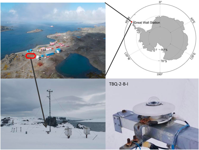
FIGURE 1. Location of the Great Wall Station in Antarctica (upper right), regional overview map (upper left), meteorological observation site (bottom left), and radiation instruments (bottom right).

2.2 Reanalysis and satellite products

2.1.1 ERA5

The ERA5 dataset is the latest reanalysis from the European Centre for Medium-Range Weather Forecasts (ECMWF) based on its previous generation ERA-Interim dataset. Compared with the previous ERA-Interim dataset, the ERA5 dataset has longer time coverage, a more accurate data assimilation system, and finer spatial resolution (Hersbach et al., 2020). ERA5 currently provides the data from 1950 to the present. The dataset chosen for the study is the monthly product (ERA5 monthly averaged data on single levels from 1959 to present), which mainly uses its downward shortwave radiation data.

2.1.2 CRA40

In May 2021, Chinese first generation of global atmospheric and land surface reanalysis (CRA) products were officially released, filling the gap in the field of global atmospheric reanalysis in China and providing comprehensive applications for various industries through the China Meteorological Data Website (http://data.cma.cn/CRA). The product is a reprocessing and analysis of historical meteorological observations using mature numerical prediction models and assimilation analysis to reproduce past atmospheric conditions, which has important applications in the fields of weather, climate, environment, ocean, and hydrology (Yu et al., 2021). This product reproduces the global three-dimensional atmospheric status from the ground to 55 km altitude since 1979. The dataset selected for this study is the daily surface radiation product with a spatial resolution of 34 km (Li et al., 2021).

2.1.3 ICDR (AVHRR)

The Climate Monitoring Satellite Application Facility (CM SAF) centers of the EUMETSAT member countries, mainly operated by the German Federal Meteorological Institute, aimed to create long time series of Climate Date Record (CDR) datasets that make CDRs applicable for climate change analysis and prediction (Urraca et al., 2017). The CLARA-A2 dataset is one of the CDRs of CM SAF. It is mainly generated by the data collected by different types of AVHRR sensors on board NOAA series satellites and MetOp polar series satellites. The CLARA-A2 dataset mainly includes cloud products, surface radiative flux products, and surface albedo products (Karlsson et al., 2017). It provides data at both daily and monthly average temporal resolutions, and the daily product is used for the surface radiation products in this study, with a spatial resolution of 0.25°*0.25°. The product is currently updated to the latest, namely, ICDR (AVHHR).

2.3 Methods

2.3.1 Empirical formula models

Meteorological elements are important factors that influence and reflect the variation of surface solar radiation (Wang et al., 2016; Zhang et al., 2017). Establishing the relationship between one or more meteorological elements as a function of surface solar radiation is the main idea of solar radiation estimation (Zeng et al., 2020; Huang et al., 2021). Several meteorological factors (such as sunshine duration, clouds, temperature, relative humidity, precipitation, water vapor content, and atmospheric turbidity) have been used in the estimation of global solar radiation, among which sunshine duration, clouds, and temperature are the most widely used meteorological factors (Wang et al., 2016; Zou et al., 2019; Mohammadi and Moazenzadeh, 2021; Mohammadi et al., 2022). However, since the physical parameters of clouds are very complex and difficult to measure, global solar radiation estimation methods based on sunshine duration and temperature data are the two most commonly used methods with high accuracy (He et al., 2018; Feng and Wang, 2021a, Feng and Wang, 2021b). The daily global solar radiation estimation models based on sunshine duration, temperature-based, and multi-meteorological parameters used in this study are shown in Table 1.

TABLE 1

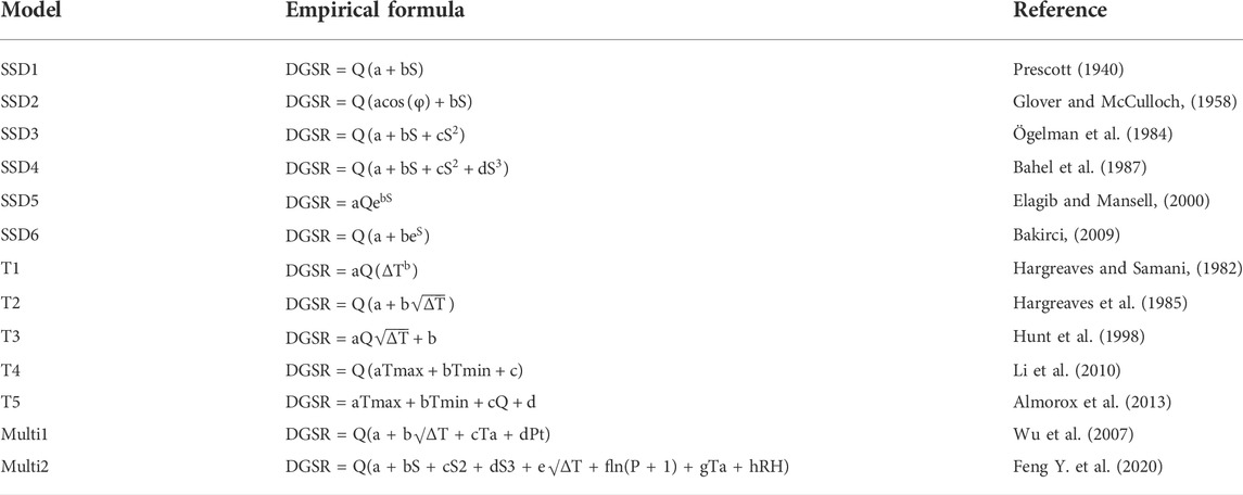
TABLE 1. Full list of predictor variables for estimating the global solar radiation

In the table, DGSR is daily global solar radiation (MJ/m²), Q is daily extraterrestrial radiation (the radiation received by the horizontal plane at the top of the atmosphere, unit: MJ/m²), S is the sunshine percentage (%), $\mathrm{\phi }$ is the geographical latitude (rad), a, b, c, d, e, f, g, and h are empirical coefficients, $\mathrm{\Delta }$ T is the daily temperature difference (°C), p is daily precipitation, ${\mathrm{P}}_{\mathrm{t}}$ is converted precipitation data, p>0, ${\mathrm{P}}_{\mathrm{t}}$ =1; p<0, ${\mathrm{P}}_{\mathrm{t}}$ =0. Here, Q can be calculated by the following formula:

$\mathrm{Q}=\frac{\mathrm{T}}{\mathrm{\pi }}{\mathrm{d}}_{\mathrm{m}}^{\mathrm{2}}\overline{{\mathrm{S}}_{\mathrm{0}}}\left({\mathrm{w}}_{\mathrm{0}}\sin \mathrm{\phi }\sin \mathrm{\delta }+\mathrm{cos\phi cos\sigma \delta sin}{\mathrm{w}}_{\mathrm{0}}\right),(1)$

where T=86,400 s, $\overline{{\mathrm{S}}_{\mathrm{0}}}$ =1367 W/m², ${\mathrm{d}}_{\mathrm{m}}^{\mathrm{2}}$ is the solar-terrestrial correction distance, ${\mathrm{w}}_{\mathrm{0}}$ is the solar hour angle, and $\mathrm{\delta }$ is the declination.

2.3.2 Machine learning models

Random forest (RF) is an extended variant of bagging. Based on the categorical regression tree as the base learner to build bagging integration, random forest further introduces the selection of random features in the training process of the decision tree (Wei et al., 2019; Zeng et al., 2020). The gradient boost regression tree (GBDT) is a boosting algorithm in which the base learner in GBDT is a categorical regression tree and each sub-model is trained based on the performance (residuals) of the trained learner (Chen et al., 2019). And a new model is built in the direction of the gradient where the residuals are reduced. GBDT can be used for most linear and nonlinear regression problems, can handle out-of-space anomalous data, and is adaptable to various types of data without requiring complex feature engineering (Chen et al., 2019). XGBoost (eXtreme Gradient Boosting) is a machine learning algorithm implemented in the gradient boosting framework. It is implemented by the gradient boosting machine and improved on the original one, which greatly improves the model training speed and prediction accuracy (Xiao et al., 2018; Xu et al., 2018; Gui et al., 2020). In the modeling process, the model may need to perform thousands of iterations for more complex data. This problem is well solved by the XGBoost model, which enables parallel operations on the regression tree. LightGBM is a decision tree-based gradient boosting framework that models complex non-linear functions. LightGBM offers distributed and high-performance advantages in sorting, classification, and regression (Zeng et al., 2021a). Other machine learning models are shown in Supplementary Text S1.

The stacking model involves the process of training a high-level learner to find the optimal combination of base learners, rather than simply fusing the results of several primary learners. Compared with bagging and boosting frameworks, which use the same type of base learners for construction, the stacking model is built by combining different types of base learners (Feng L. et al., 2020), because different types of base learners differ significantly in learning the data space and structure. Different types of base learners can observe the data features from different perspectives and learn the data more comprehensively to obtain a more accurate result (Chen et al., 2019). The core idea was to train the base learner with cross-validation, and then construct secondary features for training the meta learner based on the output of the base learner (Huang et al., 2021). Ridge regression, in essence, is a biased regression method dedicated to handling covariance data by improving the least squares method by abandoning the unbiased nature of least squares to produce biased estimates, allowing for more realistic and reliable regression coefficients at the cost of losing some information and reducing accuracy (McDonald, 2009).

In this study, the regression methods of random forest, XGBoost, and LightGBM are used as one of the base learner models for building the stacking model, and the results of the first layer are retrained and predicted using ridge regression as the second layer.

2.4 Steps of DGSR reconstruction and comparison with other products

Step 1: Data pre-processing and time matching. The daily values of the meteorological variables were obtained by averaging the four daily observations at 0000, 0600, 1200, and 1800 UTC. Daily sunshine duration and daily global solar radiation as a cumulative value for 24 h per day are obtained. The final available data include conventional meteorological observation (see Table 2) for the period 1986–2020, with radiation observations from February 2008 to December 2020.

TABLE 2

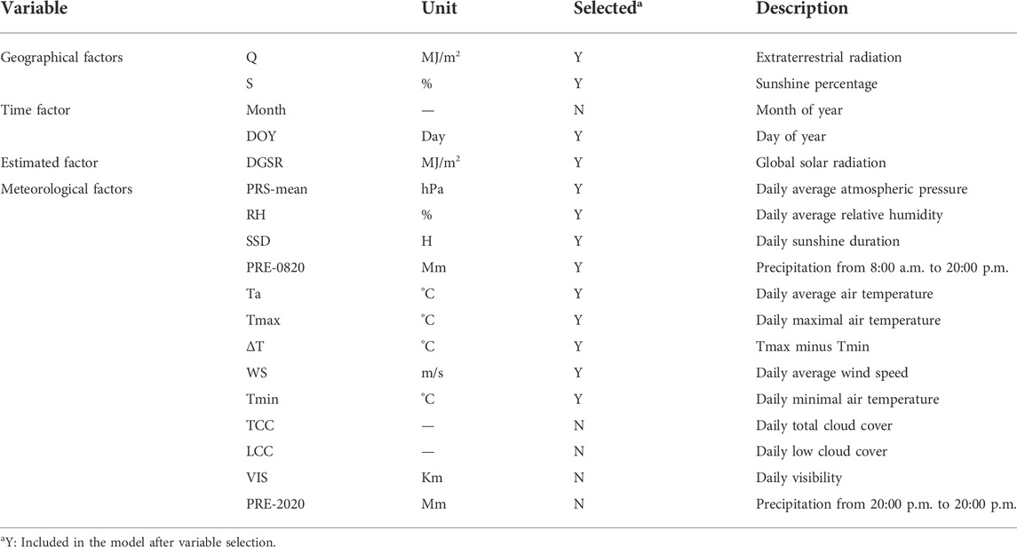
TABLE 2. Statistical information for multiple empirical formula models.

Step 2: Model construction. Empirical formula models and machine learning models are constructed based on matched samples. These empirical models include sunshine-based models (six in total), temperature-based models (five in total), and multivariate models (two in total). As in the study by Mohammadi et al. (2022), the empirical formula models were calibrated (the matched samples from 2011 to 2020 were used in this study) to obtain the empirical coefficients, and the remaining samples are then used to test the accuracy of the model (matched samples from February 2008 to December 2010 were used in this study). Machine learning models include RF, LightGBM, MLP neural networks, SVM, MLR, and stacking models. In this study, data from 2011 to 2020 were used for training and tested using a 10-fold cross-validation method (Zeng et al., 2021b). The performance of the machine learning model for historical DGSR estimation was also evaluated using data from February 2008 to December 2010. The 10-fold cross-validation method is given in Supplementary Text S2 in Supplementary Information.

Step 3: Historical dataset reconstruction. The meteorological observations of the Great Wall Station in Antarctica were used to estimate the DGSR from 1986 to 2020 in combination with the optimal model obtained in Step 2.

Step 4: Comparison with other reanalysis and satellite products. Because of the large sample size of the multi-year daily value data, we averaged the DGSR data on a monthly basis in order to visualize and explore more clearly the differences between the different DGSR products. The monthly products of the reanalysis and satellites were interpolated and time-matched to the Great Wall Station site, and then compared with the estimated DGSR, observed DGSR. Based on this reconstructed data, the annual, monthly, and seasonal variation characteristics of the DGSR at the Great Wall Station are analyzed, and the trends and their possible influencing factors are further explored.

3 Results and discussion

3.1 Empirical formula model results

Meteorological parameters (e.g., sunshine duration, temperature, and precipitation) during 2011–2020 were used as model input elements to the selected models for calculating the empirical constants. Table 3 shows that the empirical constants estimated from the SSD4 model are a=0.2474, b=0.1.3008, c=-2.1947, and d=1.5923. The empirical constants also estimated from the T3 model are a=−0.1827 and b=−0.0012. Multi2 model’s empirical constants are a=0.0780, b=1.2497, c=−2.0761, d=1.4781, e=0.0173, f=−0.0329, g=−0.0049, and h=0.0017. Details of the other model’s empirical constants are statistically provided in Table 3. The empirical constant values from different empirical formulas were used to estimate DGSR at the Great Wall Station from February 2008 to December 2010, and then a comparison between estimated DGSR and observed DGSR was made.

TABLE 3

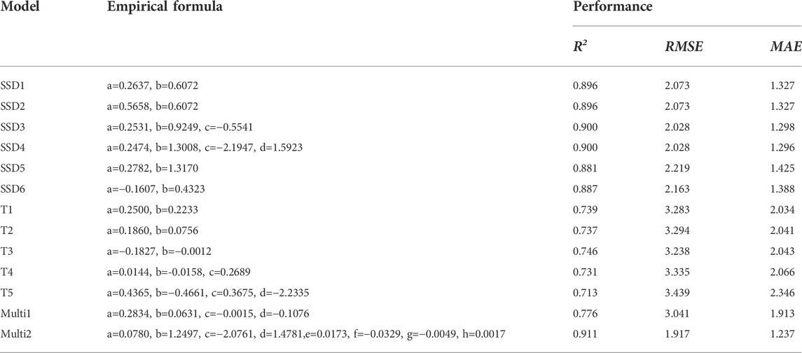
TABLE 3. Coefficients and model accuracy of the empirical formula model.

The correlation (R), standard deviation (STD), and centered root mean square difference (RMSD) between observed and estimated DGSR are plotted in Taylor diagrams (Figure 2). Figure 2 indicates temperature-based models gave relatively larger model errors than sunshine-based models. Among sunshine-based models, the SSD4 model has the highest accuracy, with the corresponding R, RMSE, and MAE of 0.949, 2.028 MJ/m², and 1.296 MJ/m², respectively. The SSD5 model had the lowest accuracy, with the values of R, RMSE, and MAE of 0.939, 2.219 MJ/m², and 1.425 MJ/m², respectively. For the temperature-based model, the T3 model had the highest accuracy (R=0.864, RMSE=3.238 MJ/m², and MAE=2.043 MJ/m²), while the T5 model had the lowest accuracy (R=0.844, RMSE=3.439 MJ/m², and MAE=2.346 MJ/m²). Other results of temperature-based models and sunshine-based models are shown in Table 3.

FIGURE 2

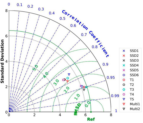
FIGURE 2. Taylor diagram of historical estimation performance for multiple empirical formula models.

The Multi1 model discussed solar radiation calculation with precipitation (${\mathrm{P}}_{\mathrm{t}}$ = 1) and no precipitation (${\mathrm{P}}_{\mathrm{t}}$ = 0). The model (parameters only include $\mathrm{\Delta T}$) was still a temperature-based model, so the low accuracy of this model can be explained in this study. The hybrid model based on multiple meteorological parameters has the highest accuracy (e.g., Multi2 with R, RMSE, and MAE are 0.955, 1.917 MJ/m², and 1.237 MJ/m², respectively), followed by the sunshine-based model, and the temperature-based model has the lowest accuracy. In general, the results showed that all empirical models were able to estimate the daily global solar radiation with high coefficients of determination and the smallest values of RMSE, MAE, and MB.

3.2 Machine learning models results

3.2.1 Variables selection and model tuning results

The RF model can select the optimal variables according to the importance of variables, thus simplifying the model. Based on “feature_importances_” parameter of the RF model in scikit-learn, the importance values of all variables can be calculated (Pedregosa et al., 2011). First, the 10-fold cross-validation results (CV R², CV RMSE, and CV MAE), hindcast test results (hindcast test R², hindcast test RMSE, and hindcast test MAE), and the importance of all variables are obtained by training the RF model. Second, the variables were sorted according to the variable’s importance from small to large, and the variable with the least importance was removed. Then, the RF model was trained again and the training results were recorded. Repeat these steps until only two input variables were left in the model.

The estimation performance of the model was evaluated according to the recorded results of each model training. When the model CV accuracy and historical prediction accuracy are both high, the corresponding training variable is determined as the final variable of the model, that is, the variable selection result. Figure 3 shows the results of model performance (CV R², CV RMSE, and CV MAE) and hindcast ability (hindcast test R², hindcast test RMSE, and hindcast test MAE) of the RF model during the variable selection process. It should be noted that steps 13 and 15, where RMSE and MAE increase dramatically, are not shown in the figure. After the sixth variable was removed (at step 6), Figure 3 indicates that the R² (CV R²=0.949, hindcast test R²=0.929) was the highest, the RMSE (CV RMSE=1.500 MJ/m², hindcast test RMSE= 1.752 MJ/m²) and MAE (CV MAE=0.930 MJ/m², hindcast test MAE=1.079 MJ/m²) were the lowest. Therefore, the remaining 11 variables were used as the final predictors, namely, Tmax, WS, PRS-mean, ΔT, S, Tmin, PRE-0820, RH, DOY, SSD, and Q. In addition, according to the results of meteorological variables correlations with DGSR (Supplementary Figure S1) and variable selection by machine learning (Figure 3), we find that the observation quality of the input variables affects the accuracy of the machine learning models because the LCC, TCC, VIS, and PRE-2020 are manually observed (which leads to human errors) at the Great Wall Station. Therefore, these variables are excluded in the variable selection process by the random forest model. This variable selection results (see Table 2) is also consistent with our previous studies (Zeng et al., 2020; Zeng et al. 2021b).

FIGURE 3

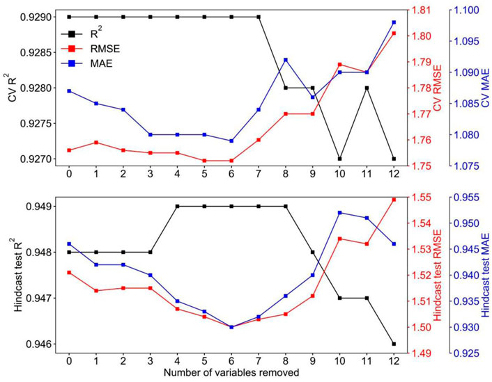
FIGURE 3. Model performance (CV R², CV RMSE, and CV MAE) and hindcast ability (hindcast test R², hindcast test RMSE, and hindcast test MAE) of the RF model during the variable selection process. The predictor variables are removed one at a time in the following order: 1) month, 2) TCC, 3) LCC, 4) VIS, 5) PRE-2020, 6) Ta, 7) Tmax, 8) WS, 9) PRS-mean, 10) ΔT, 11) S, and 12) Tmin. It should be noted that steps 13 and 15, where RMSE increases dramatically, are not shown in the figure.

Grid-search is a basic hyperparameter tuning technique, which is similar to the method of manual tuning (Siji George and Sumathi, 2020). It permutates and combines all the hyperparameter values in the model, and then builds the model according to the number of combinations. The optimal model was evaluated and selected according to the cross-validation score, and the corresponding hyperparameter combination value of the optimal model was given. The grid-search method is time-consuming and inefficient because it tries every combination of hyperparameters. The random-search method is to randomly select the hyperparameter combination from the hyperparameter space, which cannot guarantee the best parameter combination (Bergstra and Bengio, 2012). Since the machine learning model contains multiple hyperparameters, we first used the random-search method to find the potential combination of hyperparameters, and then used the grid-search method to select the optimal hyperparameters from the potential combination of hyperparameters. The range of hyperparameter tuning and the final hyperparameter combination of each machine learning model are shown in Table 4.

TABLE 4

TABLE 4. Final selection value of the main parameters in each model.

3.2.2 Comparative results of machine learning models

For the performance of machine learning models, the CV R², CV RMSE, and CV MAE of seven machine learning models are between 0.926–0.952, 1.464–1.810 MJ/m², and 0.909–1.185 MJ/m², respectively (Table 5). It shows that all models have good estimation performance. The XGBoost model had the highest overall accuracy, the CV R² value was 0.952, and the estimation uncertainty was the least. The MLP model has the same CV R² value as XGBoost, but the estimated uncertainty is relatively large (CV RMSE=1.473 MJ/m², CV MAE=0.916 MJ/m²), so the overall accuracy is lower than XGBoost. The overall accuracy of SVM was the lowest (CV R²=0.926, CV RMSE=1.810 MJ/m², and CV MAE=1.185 MJ/m²). On the fact of model performance, the model overall accuracy from high to low is as follows: XGBoost, MLP, LightGBM, GBDT, RF, MLR, and SVM.

TABLE 5

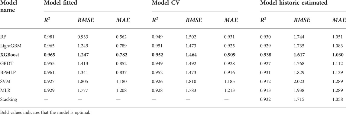
TABLE 5. Fitted, CV, and estimated results of different machine learning models.

For the historical estimation performance of machine learning, hindcast test R², hindcast test RMSE, and hindcast Test MAE are between 0.912–0.938, 1.617–2.023 MJ/m², and 1.030–1.289 MJ/m², respectively. All models show good historical estimation capability. Similarly, the XGBoost model outperforms the other six models and stacking models in historical estimation performance. The RF model and LightGBM model are second only to the stacking model, while SVM has the worst historical estimation performance. It is worth noting that compared with the RF model and LightGBM model, the MLP model and GBDT model have larger historical estimated uncertainty values. Compared with its own CV RMSE and CV MAE, hindcast test RMSE and hindcast test MAE are significantly larger, indicating the stability bias of the MLP model and GBDT model. Therefore, in the stacking model, we chose XGBoost, RF and LightGBM models as the first layer and ridge regression as the second layer. The results show that the stacking model has a high historical estimation capability (hindcast test R²=0.932, hindcast test RMSE=1.715 MJ/m², and hindcast test MAE=1.058 MJ/m²), but not the highest, second only to the XGBoost model.

Furthermore, we present XGBoost model fitting results, 10-fold CV results, and historical estimation ability results in Figure 4. Figures 4A,B shows that the XGBoost had higher R² values of 0.965 (0.952) and lower RMSE and MAE values of 1.247 MJ/m² and 0.782 MJ/m² (1.464 MJ/m² and 0.909 MJ/m²) in the model fitted (model 10-fold CV) process. The results show that the XGBoost model has high estimation accuracy and stable performance. The matched samples from February 2008 to December 2010 were used (not used in the model training and cross-validation process) to evaluate the historical estimation performance of the machine learning models, and the result of the hindcast estimated is also shown in Figure 4C. We found that the model hindcast estimated that DGSR presents a good consistency with observed DGSR (R² = 0.938, RMSE = 1.617 MJ/m², and MAE=1.030 MJ/m²). In addition, the slope (0.95, 0.94, and 0.96) and intercept (0.32, 0.38, and 0.51) corresponding to the fitted, 10-fold CV, and historical estimation ability result (R², RMSE, and MAE) have few changes, indicating that the model has good stability and generalization. Also, the XGBoost is sufficient to reconstruct the DGSR of the Great Wall Station, Antarctica.

FIGURE 4

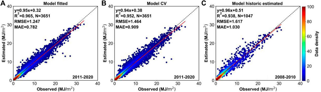
FIGURE 4. Scatterplots density of the (A) fitted model, (B) 10-fold CV model, and (C) hindcast estimation results of the XGBoost model at the Great Wall Station, Antarctica.

At the same time, the time series, frequency distribution, and difference distribution of DGSR of the Great Wall Station from February 2008 to December are also presented in Figure 5. Figure 5A shows that the time series of observed DGSR and the estimated DGSR are very consistent. Meanwhile, Figure 5B shows that the difference between the two values mainly occurs in the range of ±2 MJ/m², accounting for 83.7% of the total. Figure 5C shows that the larger the DGSR value is, the greater the difference is. Also, the samples with obvious differences are all distributed in the austral summer, which may be related to the sunshine duration, solar altitude angle, and precipitation in summer. As shown in Figure 5D, when DGSR values range from 0 to 3 MJ/m², the historical estimation performance of the model is good. With the increase of DGSR value, the historical estimation capability of the model first overestimates and then turns to underestimates. Overall, the mean difference of DGSR is 0.28 MJ/m² (very small), which also indicates that the model has extremely high historical estimation performance.

FIGURE 5

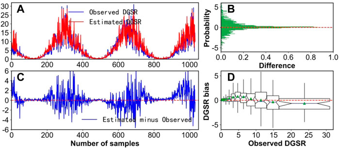
FIGURE 5. (A) Observed versus estimated DGSR, (B) probability distribution and (C) time series of the difference, and (D) DGSR bias in 2008–2010 at the Great Wall Station, Antarctica.

By comparing with the previous empirical formula models (Tables 4, 5), we found that the SVM (hindcast test R²=0.912, hindcast test RMSE=2.023 MJ/m², and hindcast test MAE=1.289 MJ/m²) and MLR (hindcast test R²=0.913, hindcast test RMSE=1.938 MJ/m², and hindcast test MAE=1.289 MJ/m²) models have comparable historical estimation performance to the Multi2 model (hindcast test R²=0.911, hindcast test RMSE=1.917 MJ/m², and hindcast test MAE=1.237 MJ/m²). Other machine learning models (especially the XGBoost model) have much higher historical estimation capacity than empirical formula models. Other studies results also show that the accuracy of estimated DGSR by machine learning models is generally higher than that of empirical formula models (Mohammadi et al., 2022).

In conclusion, the XGBoost model has stronger historical estimation ability and can be used to reconstruct the historical long time series DGSR dataset of the Great Wall Station, which is of great significance for studying the characteristics and long-term variation of surface solar radiation of the Antarctica, and exploring and understanding the reasons for its trend evolution.

3.3 Comparison with other products

To better understand the differences between the estimated DGSR and other reanalysis and satellite information, the monthly values of DGSR for each product are given in Figure 6. It can be seen that the various DGSR follow a relatively consistent trend in the time series of monthly values with the observed DGSR, both being larger in austral spring and summer and smaller in austral winter and autumn. The correlation coefficients between the estimated, ERA5, CRA40, and ICDR (AVHRR) DGSRs and the observed DGSR are 0.994, 0.982, 0.977, and 0.936, respectively. For the austral summer half-year, the estimated DGSR was agreed very well with the observed DGSR, with a mean bias of only −0.47 MJ/m². The other DGSR monthly products differ significantly from observations, with a mean bias of 3.27 MJ/m², 1.05 MJ/m², and 6.90 MJ/m² for ICDR satellite products, ERA5, and CRA40, respectively. The findings indicate that there is a high degree of uncertainty in the region for these products. The differences between them should be noted and appropriately corrected when using this information.

FIGURE 6

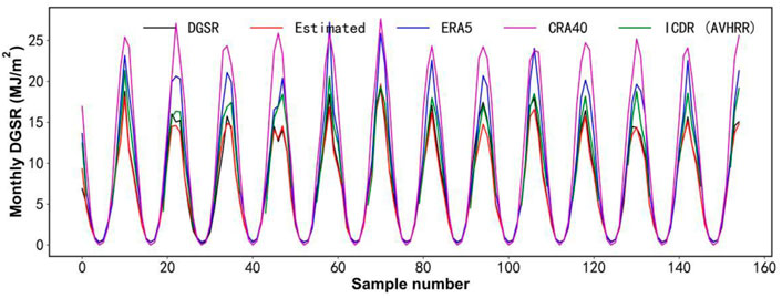
FIGURE 6. Monthly time series variation of DGSR for the Great Wall Station from February 2008 to December 2020 from multiple data sources.

The inter-year and differences (Figure 7) analysis of the DGSR for different products from 2009 to 2020 shows that the different products reflect inter-year variations in DGSR with a small range of fluctuations. From 2009 to 2020, the observed, estimated, ERA5, and CRA40 DGSRs range from 6.09 to 7.48 MJ/m², 6.30–7.15 MJ/m², 8.24–9.44 MJ/m², and 10.41–10.95 MJ/m², respectively. Figure 7B shows that the estimated DGSR differs very little from the observed values, with a negative bias (except for 2010) and a multi-year mean bias of –0.27 MJ/m². Both ERA5 and CRA40 show positive bias and large multi-year mean bias values of 1.80 MJ/m², and 3.76 MJ/m², respectively. Correspondingly, the annual relative errors of DGSR [the calculation formula of relative errors is given in Section 3.3 from Zeng et al. (2021a)] from estimated, ERA5, and CRA40 are 5.4%, 26.5% and 54.3%, respectively. It is notable that the ICDR satellite products have not been included in the DGSR annual mean comparison as the satellite has more missing measurements during the austral winter half-year.

FIGURE 7

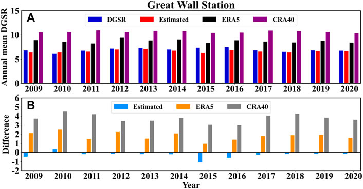
FIGURE 7. Yearly time series variation (A) and differences (B) of DGSR for the Great Wall Station during 2009–2020 from multiple data sources.

The aforementioned results show that the annual and monthly products of all the data can better reflect the characteristics of the DGSR variation at the Great Wall Station, Antarctica. Among them, the estimated DGSR in this study has a very small bias and the highest accuracy, which is sufficient to replace the observed values when the station is out of measurement. However, the DGSR of the austral summer half-year for other products [ERA5, CRA40, and ICDR (AVHRR)] deviate significantly from the observed values, and the annual averages of the DGSR deviate equally significantly. These DGSR products should be considered with caution and corrected in studies such as long-term trend evolution.

3.4 The characteristics and trends of DGSR

Annual and seasonal mean changes and trends of DGSR and multi-year monthly mean changes for the Great Wall Station, Antarctica, from 1986 to 2020 are given in Figure 8. As shown in Figure 8F, DGSR showed a decreasing and then increasing trend from January to December, with monthly average DGSR values of 13.06, 9.44, 5.47, 2.38, 0.84, 0.41, 0.59, 2.18, 5.85, 10.29, 13.57, and 15.23, respectively (Units: MJ/m²). The monthly average DGSR value (12.58 MJ/m²) was highest in austral summer (December, January, and February) and lowest (1.06 MJ/m²) in austral winter (June, July, and August). The monthly average DGSR value in austral spring (September, October, and November) was 9.90 MJ/m² and in austral autumn (March, April, and May) it was 2.90 MJ/m².

FIGURE 8

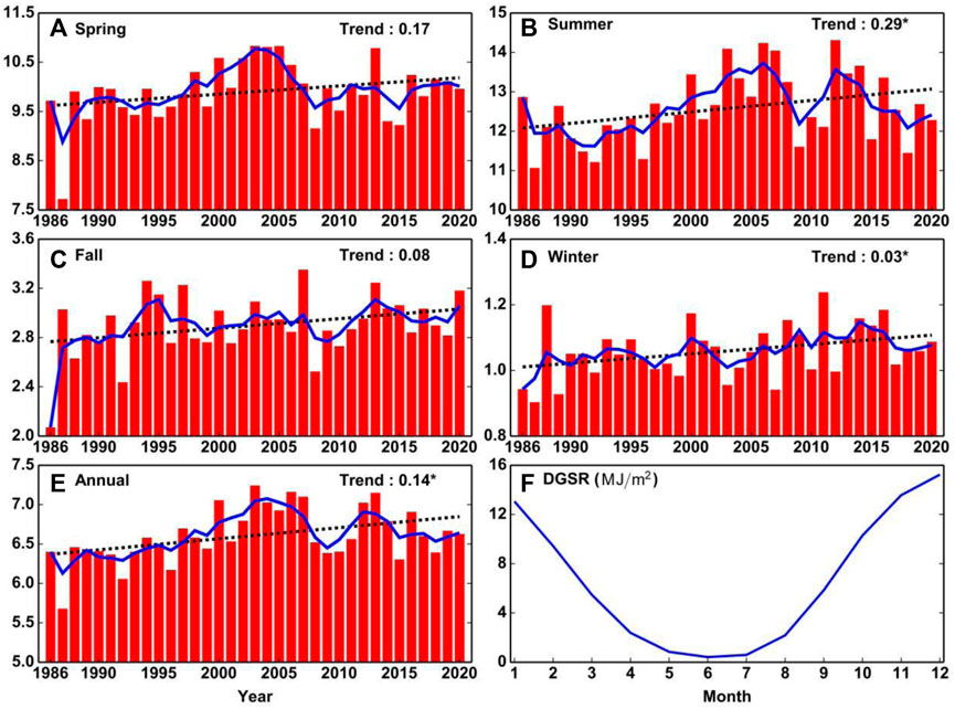
FIGURE 8. Trends in (A) spring, (B) summer, (C) autumn, (D) winter, (E) annual mean DGSR, and (F) DGSR monthly changes during 1986–2020. Star superscripts represent that the trend values of DGSR are statistically significant (p<0.05).

Figure 8E shows an increasing trend in the annual mean DGSR at the Great Wall Station over the period 1986–2020, with a trend value of 0.14 MJ/m²/decade. During the period 1990–2004, the annual mean DGSR showed an increasing trend of 0.46 MJ/m²/decade, while after 2005 the DGSR started to show a decreasing trend, which is more consistent with the trend of the Zhongshan Station, Antarctica (Zeng et al., 2021a). The annual mean DGSR value decreases slightly with a value of -0.2 MJ/m²/decade for the period 2005–2020. the reason for this phenomenon may be related to the increase in the number of precipitation days and clouds at the Great Wall station. To reveal the characteristics of the seasonal mean DGSR at Great Wall Station, we calculated the mean DGSR in spring, summer, autumn, and winter each year, and established a time series (Figures 8A–D). It can be seen that the inter-annual fluctuations in the seasonal average DGSR are large and the trend is toward an increasing trend in all four seasons. The trends in summer and winter are 0.29 MJ/m²/decade and 0.03 MJ/m²/decade, respectively, and both are statistically significant (p<0.05).

4 Conclusion

A reconstruction of the Antarctica Great Wall Station daily global solar radiation spanning 1986–2020 was presented, and is available upon request. The long-term DGSR data have the highest accuracy that agrees with the observed DGSR, and can describe the radiation characteristics and trend changes at the Great Wall Station, Antarctica. In addition, direct comparisons among ERA5, CRA40 reanalysis, and ICDR (AVHRR) satellite products were also performed in this study. The main conclusions are as follows.

Among the empirical equation models, the multi-meteorological variable model (hindcast test R², RMSE, and MAE of Multi2 are 0.911, 1.917 MJ/m², and 1.237 MJ/m², respectively) has the highest accuracy in estimating the historic DGSR at the Antarctica Great Wall Station, followed by the sunshine-based model, and the temperature-based model has the lowest accuracy (hindcast test R², RMSE, and MAE of T5 are 0.713, 3.439 MJ/m², and 2.346 MJ/m², respectively).

In the variable selection of the machine learning model, the manually observed meteorological variables have a certain impact on the model accuracy. This is mainly due to the fact that different observation crews can cause human observation errors, which in turn lead to a reduction in model accuracy. This suggests that it is important to do quality control and remove variables with poor data quality before constructing the model. All machine learning models show good historical estimation capability. The XGBoost model (hindcast test R², RMSE, and MAE are 0.938, 1.617 MJ/m², and 1.030 MJ/m², respectively) outperforms the other six models and stacking models in historical estimation performance. The RF model and LightGBM model are second only to the stacking model, while SVM has the worst historical estimation performance. In conclusion, the estimation performance of empirical formula models is generally lower than that of machine learning models. In addition, the empirical coefficients of the empirical formula model vary over time and space, require calibration using long-term radiation observations in certain regions, and cannot be generalized to other uncalibrated regions. In contrast, the machine learning model has a simple computational process, short time consumption, high simulation accuracy, and also has migration capability.

The most important result is that we found ERA5, CRA40 reanalysis, and ICDR (AVHRR) satellite products generally overestimate the DGSR, with a mean bias of 3.27 MJ/m², 6.90 MJ/m², and 1.05 MJ/m² during the austral summer half-year. The estimated DGSR, which agrees very well with the observed DGSR, has a mean bias of only −0.47 MJ/m².

In addition, the annual mean DGSR at the Great Wall Station, Antarctica over the period 1986–2020 followed a statistically significant increasing trend at a rate of 0.14 MJ/m²/decade. During the period 1990–2004, the annual mean DGSR showed an increasing trend at a rate of 0.46 MJ/m²/decade, while after 2005 the DGSR started to show a decreasing trend, which is more consistent with the trend of the Zhongshan Station, Antarctica.

Data availability statement

The raw data supporting the conclusion of this article will be made available by the authors, without undue reservation.

Author contributions

XW and MD designed the study. ZZ developed the model, performed the simulations, and analyses. ZW, WZ, DZ, KZ, and XM helped with scientific interpretation and discussion. ZZ, XW, and MD wrote the manuscript, and all authors provided input on the manuscript for revision before submission.

Funding

This work was supported by the National Natural Science Foundation of China (Nos 42122047 and 41941012), the National Basic Research Program of China (No. 2021YFC2802504), and the Basic Fund of the Chinese Academy of Meteorological Sciences (No. 2021Z006).

Conflict of interest

The authors declare that the research was conducted in the absence of any commercial or financial relationships that could be construed as a potential conflict of interest.

Publisher’s note

All claims expressed in this article are solely those of the authors and do not necessarily represent those of their affiliated organizations, or those of the publisher, the editors, and the reviewers. Any product that may be evaluated in this article, or claim that may be made by its manufacturer, is not guaranteed or endorsed by the publisher.

Supplementary material

The Supplementary Material for this article can be found online at: https://www.frontiersin.org/articles/10.3389/10.3389/feart.2022.961799/full#supplementary-material

References

Almorox, J., Bocco, M., and Willington, E. (2013). Estimation of daily global solar radiation from measured temperatures at Cañada de Luque, Córdoba, Argentina. Renew. Energy 60, 382–387. doi:10.1016/j.renene.2013.05.033

CrossRef Full Text | Google Scholar

Babar, B., Graversen, R., and Boström, T. (2018). Evaluating CM-SAF solar radiation CLARA-A1 and CLARA-A2 datasets in Scandinavia. Sol. Energy 170, 76–85. doi:10.1016/j.solener.2018.05.009

CrossRef Full Text | Google Scholar

Bahel, V., Bakhsh, H., and Srinivasan, R. (1987). A correlation for estimation of global solar radiation. Energy 12, 131–135. doi:10.1016/0360-5442(87)90117-4

CrossRef Full Text | Google Scholar

Bakirci, K. (2009). Models of solar radiation with hours of bright sunshine: A review. Renew. Sustain. Energy Rev. 13, 2580–2588. doi:10.1016/j.rser.2009.07.011

CrossRef Full Text | Google Scholar

Bergstra, J., and Bengio, Y. (2012). Random search for hyper-parameter optimization. J. Mach. Learn. Res. 13, 281–305. doi:10.1016/j.chemolab.2011.12.002

CrossRef Full Text | Google Scholar

Braun, M., and Hock, R. (2004). Spatially distributed surface energy balance and ablation modelling on the ice cap of King George Island (Antarctica). Glob. Planet. Change 42, 45–58. doi:10.1016/j.gloplacha.2003.11.010

CrossRef Full Text | Google Scholar

Brook, E. J., and Buizert, C. (2018). Antarctic and global climate history viewed from ice cores. Nature 558, 200–208. doi:10.1038/s41586-018-0172-5

PubMed Abstract | CrossRef Full Text | Google Scholar

Carrer, D., Moparthy, S., Vincent, C., Ceamanos, X., Freitas, S. C., and Trigo, I. F. (2019). Satellite retrieval of downwelling shortwave surface flux and diffuse fraction under All Sky Conditions in the framework of the LSA SAF Program (Part 2: Evaluation). Remote Sens. (Basel). 11, 2630. doi:10.3390/rs11222630

CrossRef Full Text | Google Scholar

Che, H., Zhang, X., Li, Y., Zhou, Z., and Qu, J. J. (2007). Horizontal visibility trends in China 1981-2005. Geophys. Res. Lett. 34, 247066–L24715. doi:10.1029/2007GL031450

CrossRef Full Text | Google Scholar

Che, H. Z., Shi, G. Y., Zhang, X. Y., Arimoto, R., Zhao, J. Q., Xu, L., et al. (2005). Analysis of 40 years of solar radiation data from China, 1961-2000. Geophys. Res. Lett. 32, L06803. doi:10.1029/2004GL022322

CrossRef Full Text | Google Scholar

Chen, J., Yin, J., Zang, L., Zhang, T., and Zhao, M. (2019). Stacking machine learning model for estimating hourly PM2.5 in China based on Himawari 8 aerosol optical depth data. Sci. Total Environ. 697, 134021. doi:10.1016/j.scitotenv.2019.134021

PubMed Abstract | CrossRef Full Text | Google Scholar

Ding, M., Han, W., Zhang, T., Yue, X., Fyke, J., Liu, G., et al. (2020). Towards more snow days in summer since 2001 at the great wall station, antarctic Peninsula: The role of the amundsen sea low. Adv. Atmos. Sci. 37, 494–504. doi:10.1007/s00376-019-9196-5

CrossRef Full Text | Google Scholar

Elagib, N. A., and Mansell, M. G. (2000). New approaches for estimating global solar radiation across Sudan. Energy Convers. Manag. 41, 419–434. doi:10.1016/S0196-8904(99)00123-5

CrossRef Full Text | Google Scholar

Feng, F., and Wang, K. (2021b). Merging ground-based sunshine duration observations with satellite cloud and aerosol retrievals to produce high-resolution long-term surface solar radiation over China. Earth Syst. Sci. Data 13, 907–922. doi:10.5194/essd-13-907-2021

CrossRef Full Text | Google Scholar

Feng, F., and Wang, K. (2021a). Merging high-resolution satellite surface radiation data with meteorological sunshine duration observations over China from 1983 to 2017. Remote Sens. (Basel). 13, 602. doi:10.3390/rs13040602

CrossRef Full Text | Google Scholar

Feng, L., Li, Y., Wang, Y., and Du, Q. (2020). Estimating hourly and continuous ground-level PM2.5 concentrations using an ensemble learning algorithm: The ST-stacking model. Atmos. Environ. X. 223, 117242. doi:10.1016/j.atmosenv.2019.117242

CrossRef Full Text | Google Scholar

Feng Y., Y., Gong, D., Jiang, S., Zhao, L., and Cui, N. (2020). National-scale development and calibration of empirical models for predicting daily global solar radiation in China. Energy Convers. Manag. 203, 112236. doi:10.1016/j.enconman.2019.112236

CrossRef Full Text | Google Scholar

Glover, J., and McCulloch, J. S. G. (1958). The empirical relation between solar radiation and hours of sunshine. Q. J. R. Meteorol. Soc. 84, 172–175. doi:10.1002/qj.49708436011

CrossRef Full Text | Google Scholar

Gui, K., Che, H., Zeng, Z., Wang, Y., Zhai, S., Wang, Z., et al. (2020). Construction of a virtual PM2.5 observation network in China based on high-density surface meteorological observations using the Extreme Gradient Boosting model. Environ. Int. 141, 105801. doi:10.1016/j.envint.2020.105801

PubMed Abstract | CrossRef Full Text | Google Scholar

Hargreaves, G. H., and Samani, Z. A. (1982). Estimating potential evapotranspiration. Trans. Am. Soc. Civ. Eng. 128, 324–338. doi:10.1061/taceat.0008673

CrossRef Full Text | Google Scholar

Hargreaves, G. L., Hargreaves, G. H., and Riley, J. P. (1985). Irrigation water requirements for Senegal river basin. J. Irrig. Drain. Eng. 111, 265–275. doi:10.1061/(asce)0733-9437(1985)111:3(265)(asce)0733-9437

CrossRef Full Text | Google Scholar

He, Y., Wang, K., and Feng, F. (2021). Improvement of ERA5 over ERA-interim in simulating surface incident solar radiation throughout China. J. Clim. 34, 3853–3867. doi:10.1175/JCLI-D-20-0300.1

CrossRef Full Text | Google Scholar

He, Y., Wang, K., Zhou, C., and Wild, M. (2018). A revisit of global dimming and brightening based on the sunshine duration. Geophys. Res. Lett. 45, 4281–4289. doi:10.1029/2018GL077424

CrossRef Full Text | Google Scholar

Hersbach, H., Bell, B., Berrisford, P., Hirahara, S., Horányi, A., Muñoz‐Sabater, J., et al. (2020). The ERA5 global reanalysis. Q. J. R. Meteorol. Soc. 146, 1999–2049. doi:10.1002/qj.3803

CrossRef Full Text | Google Scholar

Hock, R., De Woul, M., Radic, V., and Dyurgerov, M. (2009). Mountain glaciers and ice caps around Antarctica make a large sea-level rise contribution. Geophys. Res. Lett. 36. doi:10.1029/2008GL037020

CrossRef Full Text | Google Scholar

Huang, L., Kang, J., Wan, M., Fang, L., Zhang, C., and Zeng, Z. (2021). Solar radiation prediction using different machine learning algorithms and implications for extreme climate events. Front. Earth Sci. 9. doi:10.3389/feart.2021.596860

CrossRef Full Text | Google Scholar

Hunt, L. A., Kuchar, L., and Swanton, C. J. (1998). Estimation of solar radiation for use in crop modelling. Agric. For. Meteorol. 91, 293–300. doi:10.1016/S0168-1923(98)00055-0

CrossRef Full Text | Google Scholar

Jaross, G., and Warner, J. (2008). Use of Antarctica for validating reflected solar radiation measured by satellite sensors. J. Geophys. Res. 113, D16S34. doi:10.1029/2007JD008835

CrossRef Full Text | Google Scholar

Karlsson, K.-G., Anttila, K., Trentmann, J., Stengel, M., Fokke Meirink, J., Devasthale, A., et al. (2017). CLARA-A2: The second edition of the CM SAF cloud and radiation data record from 34 years of global AVHRR data. Atmos. Chem. Phys. 17, 5809–5828. doi:10.5194/acp-17-5809-2017

CrossRef Full Text | Google Scholar

Krähenmann, S., Obregon, A., Müller, R., Trentmann, J., and Ahrens, B. (2013). A satellite-based surface radiation climatology derived by combining climate data records and near-real-time data. Remote Sens. (Basel). 5, 4693–4718. doi:10.3390/rs5094693

CrossRef Full Text | Google Scholar

Lachlan-Cope, T. (2005). Role of sea ice in forcing the winter climate of Antarctica in a global climate model. J. Geophys. Res. 110, D03110. doi:10.1029/2004JD004935

CrossRef Full Text | Google Scholar

Li, C., Zhao, T., Shi, C., and Liu, Z. (2021). Assessment of precipitation from the CRA40 dataset and new generation reanalysis datasets in the global domain. Int. J. Climatol. 41, 5243–5263. doi:10.1002/joc.7127

CrossRef Full Text | Google Scholar

Li, M. F., Liu, H. B., Guo, P. T., and Wu, W. (2010). Estimation of daily solar radiation from routinely observed meteorological data in Chongqing, China. Energy Convers. Manag. 51, 2575–2579. doi:10.1016/j.enconman.2010.05.021

CrossRef Full Text | Google Scholar

Ma, Y., and Pinker, R. T. (2012). Modeling shortwave radiative fluxes from satellites. J. Geophys. Res. 117. doi:10.1029/2012JD018332

CrossRef Full Text | Google Scholar

McDonald, G. C. (2009). Ridge regression. WIREs. Comp. Stat. 1 (1), 93–100. doi:10.1002/wics.14

CrossRef Full Text | Google Scholar

Mohammadi, B., Moazenzadeh, R., Bao Pham, Q., Al-Ansari, N., Ur Rahman, K., Tran Anh, D., et al. (2022). Application of ERA-Interim, empirical models, and an artificial intelligence-based model for estimating daily solar radiation. Ain Shams Eng. J. 13, 101498. doi:10.1016/j.asej.2021.05.012

CrossRef Full Text | Google Scholar

Mohammadi, B., and Moazenzadeh, R. (2021). Performance analysis of daily global solar radiation models in Peru by regression analysis. Atmos. (Basel) 12, 389. doi:10.3390/atmos12030389

CrossRef Full Text | Google Scholar

Muñoz-Sabater, J., Dutra, E., Agustí-Panareda, A., Albergel, C., Arduini, G., Balsamo, G., et al. (2021). ERA5-Land: A state-of-the-art global reanalysis dataset for land applications. Earth Syst. Sci. Data 13, 4349–4383. doi:10.5194/essd-13-4349-2021

CrossRef Full Text | Google Scholar

Ögelman, H., Ecevit, A., and Tasdemiroǧlu, E. (1984). A new method for estimating solar radiation from bright sunshine data. Sol. Energy 33, 619–625. doi:10.1016/0038-092X(84)90018-5

CrossRef Full Text | Google Scholar

Oliva, M., Navarro, F., Hrbáček, F., Hernández, A., Nývlt, D., Pereira, P., et al. (2017). Recent regional climate cooling on the Antarctic Peninsula and associated impacts on the cryosphere. Sci. Total Environ. 580, 210–223. doi:10.1016/j.scitotenv.2016.12.030

PubMed Abstract | CrossRef Full Text | Google Scholar

Pattyn, F., and Morlighem, M. (2020). The uncertain future of the antarctic ice sheet. Science 367, 1331–1335. doi:10.1126/science.aaz5487

PubMed Abstract | CrossRef Full Text | Google Scholar

Pedregosa, F., Varoquaux, G., Gramfort, A., Michel, V., Thirion, B., Grisel, O., et al. (2011). Scikit-learn: Machine learning in python. J. Mach. Learn. Res. 12, 2825–2830. doi:10.48550/arXiv.1201.0490

CrossRef Full Text | Google Scholar

Prescott, J. A. (1940). Evaporation from a water surface in relation to solar radiation. Trans. Roy. Soc. Austr. 641, 114–125.

Google Scholar

Pinker, R. T., Zhang, B., and Dutton, E. G. (2005). Do satellites detect trends in surface solar radiation? Science 308, 850–854. doi:10.1126/science.1103159

PubMed Abstract | CrossRef Full Text | Google Scholar

Prăvălie, R., Patriche, C., and Bandoc, G. (2019). Spatial assessment of solar energy potential at global scale. A geographical approach. J. Clean. Prod. 209, 692–721. doi:10.1016/j.jclepro.2018.10.239

CrossRef Full Text | Google Scholar

Sanchez-Lorenzo, A., Enriquez-Alonso, A., Wild, M., Trentmann, J., Vicente-Serrano, S. M., Sanchez-Romero, A., et al. (2017). Trends in downward surface solar radiation from satellites and ground observations over Europe during 1983–2010. Remote Sens. Environ. 189, 108–117. doi:10.1016/j.rse.2016.11.018

CrossRef Full Text | Google Scholar

Scott, R. C., Lubin, D., Vogelmann, A. M., and Kato, S. (2017). West Antarctic ice sheet cloud cover and surface radiation budget from NASA A-Train satellites. J. Clim. 30, 6151–6170. doi:10.1175/JCLI-D-16-0644.1

CrossRef Full Text | Google Scholar

Sentian, J., Herman, F., Mohd Nadzir, M. S., and Wan Yee, V. K. (2020). Surface ozone variations at the great wall station, Antarctica during austral summer. Adv. Polar Sci. 31 (2), 11. doi:10.13679/j.advps.2020.0007

CrossRef Full Text | Google Scholar

Siji George, C. G., and Sumathi, B. (2020). Grid search tuning of hyperparameters in random forest classifier for customer feedback sentiment prediction. Int. J. Adv. Comput. Sci. Appl. 11. doi:10.14569/IJACSA.2020.0110920

CrossRef Full Text | Google Scholar

Soares, J., Alves, M., Dutra Ribeiro, F. N., and Codato, G. (2019). Meteorological and surface radiation data observed at the Brazilian Antarctic station on King George Island. Data Brief. 25, 104245. doi:10.1016/j.dib.2019.104245

PubMed Abstract | CrossRef Full Text | Google Scholar

Stanhill, G., and Cohen, S. (1997). Recent changes in solar irradiance in Antarctica. J. Clim. 10, 2078–2086. doi:10.1175/1520-0442(1997)010<2078:RCISII>2.0.CO;2

CrossRef Full Text | Google Scholar

Tang, W. J., Yang, K., Qin, J., Cheng, C. C. K., and He, J. (2011). Solar radiation trend across China in recent decades: A revisit with quality-controlled data. Atmos. Chem. Phys. 11, 393–406. doi:10.5194/acp-11-393-2011

CrossRef Full Text | Google Scholar

Thornton, P. E., and Running, S. W. (1999). An improved algorithm for estimating incident daily solar radiation from measurements of temperature, humidity, and precipitation. Agric. For. Meteorol. 93, 211–228. doi:10.1016/S0168-1923(98)00126-9

CrossRef Full Text | Google Scholar

Turner, J., Marshall, G. J., Clem, K., Colwell, S., Phillips, T., and Lu, H. (2020). Antarctic temperature variability and change from station data. Int. J. Climatol. 40, 2986–3007. doi:10.1002/joc.6378

CrossRef Full Text | Google Scholar

Tzallas, V., Hatzianastassiou, N., Benas, N., Meirink, J. F., Matsoukas, C., Stackhouse, P., et al. (2019). Evaluation of CLARA-A2 and ISCCP-H cloud cover climate data records over Europe with ECA&D ground-based measurements. Remote Sens. (Basel). 11, 212. doi:10.3390/rs11020212

CrossRef Full Text | Google Scholar

Urraca, R., Gracia-Amillo, A. M., Koubli, E., Huld, T., Trentmann, J., Riihelä, A., et al. (2017). Extensive validation of CM SAF surface radiation products over Europe. Remote Sens. Environ. 199, 171–186. doi:10.1016/j.rse.2017.07.013

PubMed Abstract | CrossRef Full Text | Google Scholar

van den Broeke, M., Reijemer, C., and van de Wal, R. (2004). Surface radiation balance in Antarctica as measured with automatic weather stations. J. Geophys. Res. 109, D09103. doi:10.1029/2003JD004394

CrossRef Full Text | Google Scholar

Wang, L., Kisi, O., Zounemat-Kermani, M., Salazar, G. A., Zhu, Z., and Gong, W. (2016). Solar radiation prediction using different techniques: Model evaluation and comparison. Renew. Sustain. Energy Rev. 61, 384–397. doi:10.1016/j.rser.2016.04.024

CrossRef Full Text | Google Scholar

Wang, Y., Trentmann, J., Yuan, W., and Wild, M. (2018). Validation of CM SAF CLARA-A2 and SARAH-E surface solar radiation datasets over China. Remote Sens. (Basel). 10, 1977. doi:10.3390/rs10121977

CrossRef Full Text | Google Scholar

Wei, J., Huang, W., Li, Z., Xue, W., Peng, Y., Sun, L., et al. (2019). Estimating 1-km-resolution PM2.5 concentrations across China using the space-time random forest approach. Remote Sens. Environ. 231, 111221. doi:10.1016/j.rse.2019.111221

CrossRef Full Text | Google Scholar

Wild, M., Gilgen, H., Roesch, A., Ohmura, A., Long, C. N., Dutton, E. G., et al. (2005). From dimming to brightening: Decadal changes in solar radiation at earth’s surface. Science 308, 847–850. doi:10.1126/science.1103215

PubMed Abstract | CrossRef Full Text | Google Scholar

Wild, M. (2009). Global dimming and brightening: A review. J. Geophys. Res. 114, D00D16. doi:10.1029/2008JD011470

CrossRef Full Text | Google Scholar

Wu, G., Liu, Y., and Wang, T. (2007). Methods and strategy for modeling daily global solar radiation with measured meteorological data - a case study in Nanchang station, China. Energy Convers. Manag. 48, 2447–2452. doi:10.1016/j.enconman.2007.04.011

CrossRef Full Text | Google Scholar

Xiao, Q., Chang, H. H., Geng, G., and Liu, Y. (2018). An ensemble machine-learning model to predict historical PM2.5 concentrations in China from satellite data. Environ. Sci. Technol. 52, 13260–13269. doi:10.1021/acs.est.8b02917

PubMed Abstract | CrossRef Full Text | Google Scholar

Xu, Y., Ho, H. C., Wong, M. S., Deng, C., Shi, Y., Chan, T. C., et al. (2018). Evaluation of machine learning techniques with multiple remote sensing datasets in estimating monthly concentrations of ground-level PM2.5. Environ. Pollut. 242, 1417–1426. doi:10.1016/j.envpol.2018.08.029

PubMed Abstract | CrossRef Full Text | Google Scholar

Yang, K., Huang, G. W., and Tamai, N. (2001). A hybrid model for estimating global solar radiation. Sol. Energy 70, 13–22. doi:10.1016/S0038-092X(00)00121-3

CrossRef Full Text | Google Scholar

Yang, Q., Yin, Z., Zhang, L., Xing, J., and Su, B. (2010). A case study on snow storm at great wall station, Antarctica. Chin. J. POLAR Res. 22, 141–149. doi:10.3724/sp.j.1084.2010.00141

CrossRef Full Text | Google Scholar

Yang, Q., Yu, L., Wei, L., Zhang, B., and Meng, S. (2013). Features of visibility variation at great wall station, Antarctica. Adv. Polar Sci. 24, 188. doi:10.3724/sp.j.1085.2013.00188

CrossRef Full Text | Google Scholar

Yu, L., Yang, Q., Zhou, M., Lenschow, D. H., Wang, X., Zhao, J., et al. (2019). The variability of surface radiation fluxes over landfast sea ice near Zhongshan station, east Antarctica during austral spring. Int. J. Digit. Earth 12, 860–877. doi:10.1080/17538947.2017.1304458

CrossRef Full Text | Google Scholar

Yu, X., Zhang, L., Zhou, T., and Liu, J. (2021). The asian subtropical westerly jet stream in CRA-40, ERA5, and CFSR reanalysis data: Comparative assessment. J. Meteorol. Res. 35, 46–63. doi:10.1007/s13351-021-0107-1

CrossRef Full Text | Google Scholar

Zeng, Z., Gui, K., Wang, Z., Luo, M., Geng, H., Ge, E., et al. (2021a). Estimating hourly surface PM2.5 concentrations across China from high-density meteorological observations by machine learning. Atmos. Res. 254, 105516. doi:10.1016/j.atmosres.2021.105516

CrossRef Full Text | Google Scholar

Zeng, Z., Wang, Z., Ding, M., Zheng, X., Sun, X., Zhu, W., et al. (2021b). Estimation and long-term trend analysis of surface solar radiation in Antarctica: A case study of zhongshan station. Adv. Atmos. Sci. 38, 1497–1509. doi:10.1007/s00376-021-0386-6

CrossRef Full Text | Google Scholar

Zeng, Z., Wang, Z., Gui, K., Yan, X., Gao, M., Luo, M., et al. (2020). Daily global solar radiation in China estimated from high‐density meteorological observations: A random forest model framework. Earth Space Sci. 7. doi:10.1029/2019EA001058

CrossRef Full Text | Google Scholar

Zhang, J., Zhao, L., Deng, S., Xu, W., and Zhang, Y. (2017). A critical review of the models used to estimate solar radiation. Renew. Sustain. Energy Rev. 70, 314–329. doi:10.1016/j.rser.2016.11.124

CrossRef Full Text | Google Scholar

Zhang, S. Q., Ren, G. Y., Ren, Y. Y., Zhang, Y. X., and Xue, X. Y. (2021). Comprehensive evaluation of surface air temperature reanalysis over China against urbanization-bias-adjusted observations. Adv. Clim. Change Res. 12, 783–794. doi:10.1016/j.accre.2021.09.010

CrossRef Full Text | Google Scholar

Zhang, T., Zhou, C., and Zheng, L. (2019). Analysis of the temporal–spatial changes in surface radiation budget over the Antarctic sea ice region. Sci. Total Environ. 666, 1134–1150. doi:10.1016/j.scitotenv.2019.02.264

PubMed Abstract | CrossRef Full Text | Google Scholar

Zou, L., Wang, L., Li, J., Lu, Y., Gong, W., and Niu, Y. (2019). Global surface solar radiation and photovoltaic power from Coupled Model Intercomparison Project Phase 5 climate models. J. Clean. Prod. 224, 304–324. doi:10.1016/j.jclepro.2019.03.268

CrossRef Full Text | Google Scholar