Modeling of soil–rock mixture landslides with the generalized interpolation material point method

Introduction

The soil–rock mixture (SRM) slope is a common slope type in nature, which is mainly composed of rock and soil with significant differences in properties (Yue and Morin, 1996). In southwest China, the development of water resources and the construction of many water conservancy facilities resulted in the formation of a more widely distributed reservoir bank slope, including a large number of slopes belonging to the SRM slope. Under the action of reservoir water soaking, wave scouring, and reservoir fluctuation, the weathering degree of rock and soil increases, the shear strength decreases, and then is destroyed, which poses a severe threat to water conservancy facilities and the lives and property of nearby residents.

The research method of the SRM slope is very distinct from that of the homogeneous slope (He and Kusiak, 2018; Li et al., 2021a; Zhou et al., 2021), and the typical methods often encounter great challenges in this problem (Li et al., 2021b; Cui et al., 2021; Li et al., 2022). Previous studies on SRM have focused on shear strength (Springman et al., 2003; Cen et al., 2017; Zhang et al., 2016), permeability characteristics (Yilmaz et al., 2012; Tang et al., 2015), and determining the reliability and failure risk of SRM slopes (Yang et al., 2019; Napoli et al., 2021). The spatial distribution, content, and particle size of block stones greatly influence the shear strength characteristics of the SRM. When the stone particle size is small, and the content is small, it has little effect on the shear performance. When the rock reaches a specific size and content, it becomes an essential factor affecting the mechanical properties of SRM. The permeability of SRM increases with the increase of fragment content, but the permeability of fractured rock mass with incomplete disintegration is relatively low. In the stability research of SRM slope, the digital image processing technology is usually used to establish the SRM slope model. Then the finite element method (FEM) is used for simulation analysis. The current analysis results show that the SRM slope is difficult to form the sliding surface from the slope toe to the slope top, and the rock mass has a particularly positive impact on the stability of the SRM slope.

The idea of this article is to study the dynamic evolution of unstable SRM slope landslide by means of numerical simulation, which is helpful for us to find out the dynamic characteristics of SRM slope when large deformation and failure occurs, the influence of stones on it during the landslide process and the accumulation characteristics that finally reach the stable state.

The numerical method used in this article is the material point method (MPM). The MPM (Mast 2013; Guide 2019) was proposed by Sulsky et al. (1994). They changed the constitutive equation to the calculation on the material point (MP), so the fluid in particle (FLIP) method is extended to the solid mechanics problem, and the MPM framework is established. It employs a Eulerian background grid and Lagrangian particle dual description; all the information is carried by the MP, the control equation is solved on the background grid, and the shape function is used to map the information between them. The grid will be reestablished at each time, which effectively avoids the numerical solution caused by grid distortion. Therefore, the MPM has excellent advantages in solving large deformation problems. In the past few years, MPM has been applied to the research of many physical problems, including explosion problems (Cui et al., 2013), high-speed impact problems (Liu et al., 2015; Liu et al., 2016; Ye et al., 2018) and the analysis of granular materials (Jiang et al., 2020). The application of MPM in geotechnical problems includes landslide (Andersen and Andersen, 2010; Liu et al., 2018; Ying et al., 2021), dam failure (Zabala and Alonso, 2012; Zhao et al., 2017), debris flow (Zhang and Jayaraman, 2013) and rock cracking (Nairn and Guo, 2005).

MPM has many similarities with other numerical methods, such as the particle finite element method (PFEM), smoothed particle hydrodynamics method (SPH), and discrete element method (DEM). Ye et al. (2018) conducted a detailed comparative discussion on the similarities and differences of these methods. The original MP method adopts a piecewise linear shape function, and its gradient is discontinuous at the grid boundary, resulting in the numerical oscillation of the MP when crossing the grid. In 2004, Bardenhgen and Kober extended the MPM based on the Petrov–Galerkin method and proposed the generalized interpolation material point method (GIMP), which improved the smoothness of shape function and effectively suppressed the stress oscillation of MPM (Bardenhagen and Kober, 2004). GIMP is adopted in this article, and the specific simulation procedure is as follows:

• Determine the initial state of the SRM slope.

• Trigger landslide.

• Simulate the dynamic evolution process of the sliding body.

The explicit time integration scheme is adopted in the simulation, and the Jaumann stress rate tensor is used to ensure the objective stress rate (Chen and Brannon, 2002; Zhang et al., 2016). The constitutive characteristics of soil are described by the elastic-plastic material model based on the D-P yield criterion. In order to make the simulation process more stable, this article adopts a minor time step and a stable momentum mapping scheme. Based on the aforementioned numerical methods, the dynamic evolution characteristics of homogeneous soil slope and SRM slope are compared. Under the same stone content, the influence of the shape and size of block stones on the landslide is studied.

MPM and GIMP

Like the FEM, the MPM is also a numerical method based on the Galerkin framework, so some scholars regard it as a variant of the FEM (Wang et al., 2016). The most significant difference between MPM and FEM is that MPM uses two systems of MPs and a background grid to describe the simulated object (Mast, 2013), but it should be pointed out that the status of MPs and background grid is different. MPs occupy a dominant position, and all the information is stored on the MPs. Unlike SPH and DEM, these MPs are only the integral point of the control equation in space and do not represent the actual particles. The grid occupies a secondary position and is mainly used to solve the control equation. The information mapping between the MPs and the grid is controlled by the shape function built on the background grid node (Jiang et al., 2020).

Governing equation and discretization

Before discussing GIMP, we briefly discuss the original MPM. MPs always carry mass information and will not be lost, so the MPM inherently meets the mass conservation. In this study, the heat exchange is not considered, so the energy conservation law is also satisfied. To sum up, the system’s state can be determined only by solving the momentum equation. Based on the updated Lagrangian scheme, the momentum equation of the continuum can be expressed as

$\rho {\ddot{u}}_i={\sigma }_{ij,j}+\rho b_i,(1)$

where $\rho$ represents the current mass density of the material, $u_i$ represents the displacement, ${\sigma }_{ij}$ represents the Cauchy stress, the superscript represents the time derivative, the subscript represents the component of the tensor, the partial derivative, and $b_i$ represents the volume force of unit mass, such as gravity.

The momentum Equation 1 needs to be satisfied in the current configuration of the continuum, and the boundary conditions are

$\{\begin{array}{l}\left(n_j{\sigma }_{ij}\right)|{\mathrm{\Gamma }}_t=\overline{t_i},\hfill \\ v_i|{\mathrm{\Gamma }}_u=\overline{v_i},\hfill \end{array}(2)$

where ${\Gamma }_t$ and ${\Gamma }_u$ represent the given surface force boundary and the given displacement boundary, respectively, $n_j$ is the unit vector of the outer normal of boundary ${\Gamma }_t$, ${\overline{t}}_i$ is the surface force acting on the boundary ${\Gamma }_t$, and ${\overline{v}}_i$ is the velocity of the displacement boundary ${\Gamma }_u$.

According to the principle of virtual displacement and the technique of partial integration, a weak form of governing equation can be obtained:

${\displaystyle {\int }_{\mathrm{\Omega }}\rho }{\ddot{u}}_i\delta u_{i}dV+{\displaystyle {\int }_{\mathrm{\Omega }}\rho }{\sigma }_{ij}^s\delta u_{i,j}dV-{\displaystyle {\int }_{\mathrm{\Omega }}\rho }{b}_i\delta u_{i}dV-{\displaystyle {\int }_{{\mathrm{\Gamma }}_{\mathrm{t}}}\rho }{\overline{t}}_i^s\delta u_{i}dA=\text{0,}(3)$

where $\delta u_i$ represents a virtual displacement equal to 0 on ${\Gamma }_u$, ${\sigma }_{ij}^s={\sigma }_{ij}/\rho$ represents specific stress, and ${\overline{t}}_i^s={\overline{t}}_i/\rho$ represents the boundary surface force.

As shown in Figure 1, the region $\Omega$ is discretized into blue MPs, and the density of the continuum can be approximated as

$\rho \left(x_i\right)={\displaystyle \sum _p{m}_p\delta (x_i-x_{ip})},(4)$

where $\delta$ is the Dirac-delta function, $m_p$ represents the mass of the MP $p$, and $x_{ip}$ is the coordinate of the MP $p$. As a result, Equation 3 can be transformed into a particle summation form.

${\displaystyle \sum _p{m}_p}{\ddot{u}}_{ip}\delta u_{ip}+{\displaystyle \sum _p{m}_p}{\sigma }_{ijp}^s\delta u_{ip}-{\displaystyle \sum _p{m}_p}{b}_{ip}\delta u_{ip}-{\displaystyle \sum _p{m}_p}{\overline{t}}_{ip}^s{h}^{-1}\delta u_{ip}=0,(5)$

where the subscript $p$ denotes the physical quantity carried by the MP at the $x_{ip}$ position, and $h$ is the imaginary boundary layer thickness introduced to transform the last item at the left end of Equation 3 into volume integral.

FIGURE 1

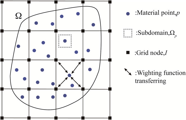
FIGURE 1. Discrete diagram of material point method.

In each calculation step of the MPM, the MP and the background grid are fixed together, so the information mapping can be realized by interpolating the shape function $N_I\left(x_i\right)$ established on the background grid node, and the variables on the background grid node are represented by the quantity with a subscript $I$. The displacement $u_{ip}$ and virtual displacement $\delta u_{ip}$ of the MPs can be expressed as

$u_{ip}=N_{Ip}{u}_{iI},(6)$

$\delta u_{ip}=N_{Ip}\delta u_{iI},(7)$

where $N_{Ip}$ represents the value of the shape function of the grid node I at the MP. In two-dimensional problems, the background grid of the original MPM usually adopts a regular four-node plane element, and its shape function is always a piecewise linear shape function

$N_{Ip}=\frac{1}{4}(1+{\xi }_I{\xi }_p)(1+{\eta }_I{\eta }_p),I=\mathrm{1,2,3,4}(8)$

in the equation, ${\xi }_p$ and ${\eta }_p$ denote the natural coordinates of the MPs, ${\xi }_I$ and ${\eta }_I$ are the natural coordinates of the grid node.

According to Equations 6, 7, the motion equation of the background grid can be rewritten as

${\dot{p}}_{iI}=f_{iI}^{int}+f_{iI}^{ext},x_I\notin {\mathrm{\Gamma }}_u,(9)$

$p_{iI}=m_I{\dot{u}}_{iI},(10)$

$f_{iI}^{int}=-{\displaystyle \sum _p{N}_{Ip,j}}{\sigma }_{ijp}\frac{m_p}{{\rho }_p},(11)$

$f_{iI}^{ext}={\displaystyle \sum _p{N}_{Ip}}{m}_p{b}_{ip}+{\displaystyle \sum _p{N}_{Ip}}\frac{m_p}{{\rho }_p}{\overline{t}}_{ip}{h}^{-1}\frac{m_p}{{\rho }_p},(12)$

where $p_{iI}$ represents the momentum of the background grid node $I$ in the $i$ direction. For simplicity, $m_I$ adopts the lumped mass matric. $f_{iI}^{int}$ and $f_{iI}^{ext}$ represent the internal force and external force of node $I$ in the $i$ direction, respectively.

Considering that the computational domain $\mathrm{\Omega }$ is time-varying, Equation 9 must be satisfied at each time step; the continuous-time is discretized by the central difference method

$p_{iI}^{n+1/2}=p_{iI}^{n-1/2}+f_{iI}^n\mathrm{\Delta }t,(13)$

where $\mathrm{\Delta }t$ represents the increment of each time step, which is a fixed value in this article, the superscript n represents the time step and $f_{iI}^n=f_{iI}^{int}+f_{iI}^{ext}$.

From MPM to GIMP

The original MPM always experiences the cell crossing error (Guide, 2019), which leads to incorrect simulation results. GIMP can effectively overcome this error. Compared with the SPH method, it introduces particle characteristic function to expand the integration area of particle variable. When the MPs pass through the boundary of the background grid, the integration of particle variables can remain continuous. As shown in Figure 2A, $L_p$ represents the partition of the total domain $\Omega$ occupied by an MP, so the MP is not associated with a point, but with an interval. Figure 2B shows the distribution of the contribution of the MP to the background grid in the same configuration. At this time, the MP contributes to two adjacent grids, so the grid intersects, that is, the influence domain of the shape function is larger than that of a grid space. Compared with the piecewise linear shape function, the MP is not only associated with one background grid (de Vaucorbeil et al., 2020).

FIGURE 2

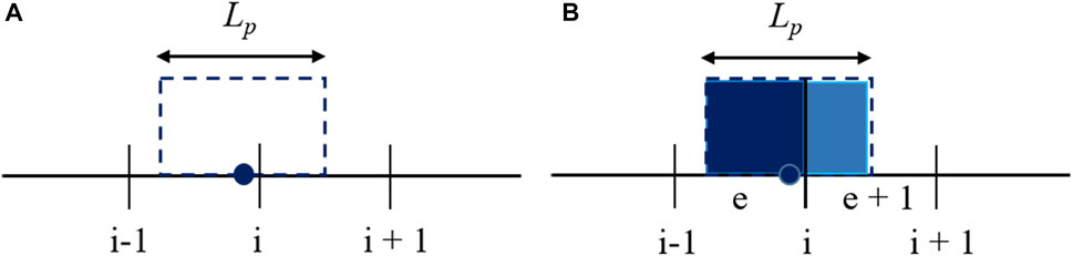
FIGURE 2. (A) Characteristic function ${\chi }_p\left(x\right)$ for one MP. (B) Treating the grid-crossing problem in GIMP.

The characteristic function of the MP satisfies the unit decomposition condition, so it can ensure that the physical quantity is conserved in the simulation process. When the characteristic function is equal to the Dirac Delta function, GIMP is equivalent to MPM. In this article, the characteristic function is

${\chi }_p\left(x_{ip}\right)=\{\begin{array}{cc}1,& \mathrm{if}x\in {\mathrm{\Omega }}_p,\\ 0,& \mathrm{else}\mathrm{.}\end{array}(14)$

Characteristic function (14) is a simple example, which can be defined as the unit partition of the initial configuration. This GIMP technique is called continuous particle GIMP or cpGIMP. Weight functions $S_{Ip}$ and their gradient functions $S_{Ip,j}$ are shown in Equations 15, 16.

$S_{Ip}=\frac{1}{V_p}{\displaystyle {\int }_{{\mathrm{\Omega }}_p\cap \mathrm{\Omega }}\chi \left(x_{ip}\right)N_{Ip}\left(x_{ip}\right)dx},(15)$

$S_{Ip,j}=\frac{1}{V_p}{\displaystyle {\int }_{{\mathrm{\Omega }}_p\cap \mathrm{\Omega }}\chi \left(x_{ip}\right)N_{Ip,j}\left(x_{ip}\right)dx},(16)$

where $V_p={\displaystyle {\int }_{\mathrm{\Omega }}{\chi }_p\left(x_{ip}\right)d\mathrm{\Omega }}$ represents the volume of an MP. Equation 5 can be rewritten as Equation 17 by applying Equations 15, 16.

${\displaystyle \sum _p{\displaystyle {\int }_{{\mathrm{\Omega }}_p\cap \mathrm{\Omega }}\frac{m_p{\ddot{u}}_{ip}}{V_p}{\chi }_p\delta u_{ip}d\mathrm{\Omega }}}+{\displaystyle \sum _p{\displaystyle {\int }_{{\mathrm{\Omega }}_p\cap \mathrm{\Omega }}{m}_p\frac{{\sigma }_{ijp}^s}{V_p}{\chi }_p\delta u_{ip}d\mathrm{\Omega }}}-{\displaystyle \sum _p{\displaystyle {\int }_{{\mathrm{\Omega }}_p\cap \Omega }\frac{m_p}{V_p}{b}_{ip}{\chi }_p\delta u_{ip}d\mathrm{\Omega }}}-{\displaystyle \sum _p{\displaystyle {\int }_{\partial \mathrm{\Omega }}\frac{m_p}{V_p}}{\overline{t}}_{ip}^s{\chi }_p{h}^{-1}\delta u_{ip}d\mathrm{\Gamma }=0}.(17)$

The displacement $u_{ip}$ and virtual displacement $\delta u_{ip}$ of the MPs can also be obtained by interpolating the background grid nodes according to the weight function $S_{Ip}$.The solution of the momentum equation is the same as that of the original MPM, but GIMP provides a more smooth weight function, and specifically, $S_{Ip,j}$ has C¹ continuity. It should be pointed out that since the influence domain of $S_{Ip,j}$exceeds one grid, the farthest grid that the MPs can influence should be considered when applying boundary conditions.

Time integration scheme

In this article, the update-stress-first (USF) format with good energy conservation is used for stress updating (Zhang et al., 2016; Guide 2019), and the detailed time integration schemes are as follows:

1) The weight function $S_{Ip}$ is used to map the mass and momentum of the MPs to the corresponding background grid node and then the node speed $v_{Ii}$ is solved:

$m_I^n={\displaystyle \sum _p{m}_p{S}_{Ip}^n},(18)$

$P_{iI}^{n-1/2}={\displaystyle \sum _p{S}_{Ip}^n{m}_p{v}_{ip}^{n-1/2}},(19)$

$v_{iI}^{n-1/2}=\frac{p_{iI}^{n-1/2}}{m_I^n}.(20)$

2) Strain rate ${\dot{\epsilon }}_{ijp}^{n-1/2}$ and rotation rate ${\Omega }_{ijp}^{n-1/2}$ of MPs are solved according to node velocity and then the mass density is updated:

${\dot{\epsilon }}_{ijp}^{n-1/2}={\displaystyle \sum _I\frac{1}{2}\left(S_{Ip,j}^n{v}_{iI}^{n-1/2}+S_{Ip,i}^n{v}_{jI}^{n-1/2}\right)},(21)$

${\mathrm{\Omega }}_{ijp}^{n-1/2}={\displaystyle \sum _I\frac{1}{2}\left(S_{Ip,j}^n{v}_{iI}^{n-1/2}-S_{Ip,i}^n{v}_{jI}^{n-1/2}\right)},(22)$

${\rho }_p^{n+1}={\rho }_p^n/\left(1+{\dot{\epsilon }}_{ijp}^{n-1/2}\mathrm{\Delta }t\right).(23)$

The elastic test stress is calculated by the elastic constitutive model:

${\tilde{\sigma }}_{ijp}^n={\sigma }_{ijp}^{n-1}+{\dot{\sigma }}_{ijp}^{n-1/2}\mathrm{\Delta }t.(24)$

The stress rate is calculated by the following equations:

$\begin{array}{cc}{\dot{\sigma }}_{ij}={\sigma }_{ij}^{\nabla }+{\sigma }_{ik}{\mathrm{\Omega }}_{jk}+{\sigma }_{jk}{\mathrm{\Omega }}_{ik},& {\sigma }_{ij}^{\nabla }=C_{ijkl}^{\sigma J}{\dot{\epsilon }}_{kl}\end{array},(25)$

where ${\sigma }_{ij}^{\nabla }$ is the Johman stress rate and $C_{ijkl}^{\sigma J}$ is the elastic stiffness tensor. Using the return mapping algorithm, the test stress is brought into the D-P criterion and the stress beyond the yield surface is pulled back to the yield surface to obtain the true stress ${\sigma }_{ijp}^n$.

3) The internal and external forces of nodes are calculated according to Equations 11, 12, and the node momentum is updated according to Equation 9. The weight function $S_{Ip}$ is used for the calculation.

4) The updated momentum is mapped back to the MP, and the hybrid momentum mapping scheme is adopted in this article, namely the mixture of PIC (particle in cell) and FLIP schemes due to the FLIP scheme experiences relatively strong numerical instability, and the momentum dissipation of the pure PIC scheme is very serious (Mast 2013; Zhang and Jayaraman, 2013).

$v_{ip}^{n+1/2}=\alpha {\displaystyle \sum _I{P}_I^{n+1/2}{S}_{Ip}^n/m_I^n}+\left(1-\alpha \right)\left(v_{ip}^{n-1/2}+\mathrm{\Delta }t{\displaystyle \sum _I{f}_{iI}^n{S}_{Ip}^n/m_I^n}\right).(26)$

The range of $\alpha$ is [0, 1]. When the values at both ends are taken, they represent the pure FLIP format or the pure PIC format, respectively. Generally, 0.01 for $\alpha$ can obtain better numerical stability and keep momentum conservation.

Model setup

In this article, four types of slopes are established, as shown in Figure 3. They are pure soil slopes, SRM slopes with arbitrary shape stones, SRM slopes with round stones, and SRM slopes with oval stones. The diameter of round stones is 0.54 m, and the long and short axes of oval stones are 0.86 and 0.34 m, respectively. The stone content of the three kinds of SRM slope is the same, 18%. The shape of the block stone mainly considers the three situations of irregular rock in nature, round and oval pebbles formed by long-term scouring by flowing water. In order to make the results more analytical, the initial position of the blocks are the same as possible when the models are established. The specific material parameters are shown in Table 1.

FIGURE 3

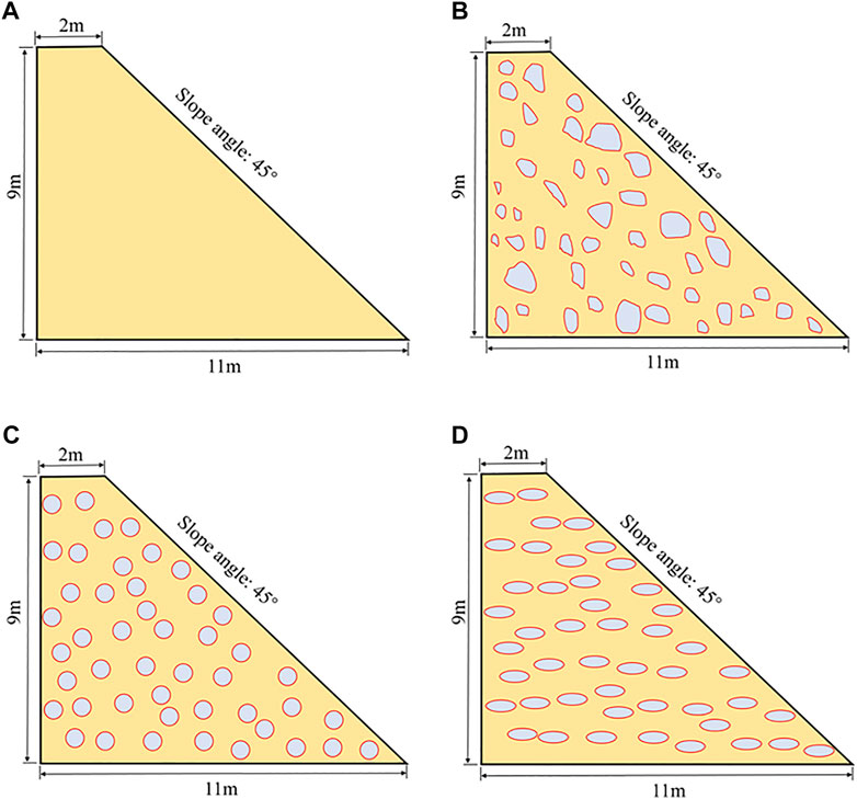
FIGURE 3. Digital model of soil slope and SRM slope. (A) Soli slope. (B) SRM slope with arbitrary shapes of stones. (C) SRM slope with round stones. (D) SRM slope with oval stones.

TABLE 1

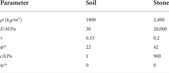
TABLE 1. Material parameters for the SRM slope.

The background grid size is 0.1 m, and four MPs are arranged in each grid. The spacing of each MP is 0.05 m, with a total of 23,490 MPs. The number of MPs of soil and rocks in the soil-rock mixture slope is 19,090, and 4,400, respectively. The time step is 0.01 ms, simulating 100,000-time steps, a total of 10 s. Before the simulation starts, the gravity is linearly loaded, and the linear elastic model is employed to update the stress; until the linear stage is completed, the dynamic damping is applied to make the kinetic energy of the slope return to 0 so as to obtain the initial state of the slope model. The essential boundary condition is applied on the left side of the model, the Coulomb friction boundary is applied on the bottom, and the friction coefficient is 0.2.

Dynamic evolution analysis

According to the simulation results, three aspects of the SRM slopes and homogeneous soil slope are compared and analyzed in this section. In Sections 4.1–4.3, we analyze the kinetic energy variation and the velocity distribution, the equivalent plastic deformation, the final configuration, and maximum sliding distance in the process of slope failure.

The kinetic energy and rate

The kinetic energy curves of homogeneous soil slope and SRM slopes during the failure process are shown in Figure 4. Overall, although the nature of the slopes is different, the duration of the landslide is the same, about 4 s; from the kinetic energy curve, the landslide can be divided into accelerated sliding, deceleration sliding, and stable stage. The acceleration time of SRM slope with round stones is the shortest, only 1.5 s. The acceleration time of SRM slope with arbitrary shapes stones is the most extended, 2s. Correspondingly, the longest and shortest deceleration stages are the SRM slope with round stones and the SRM slope with arbitrary stones.

FIGURE 4

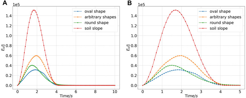
FIGURE 4. Kinetic energy curve. (A) Kinetic energy curve during simulation. (B) 0 ∼ 5s apparent kinetic energy curve.

The highest peak kinetic energy is the homogeneous soil slope, followed by the SRM slope (arbitrary shape stones). The former is about 2.5 times that of the latter, and it should be noted that the mass of the homogeneous soil slope is less than that of the SRM slopes. Therefore, the variation of the kinetic energy of homogeneous soil slope is very violent. Comparing the peak kinetic energy of the SRM slopes, it can be found that the SRM slope with oval stones is the smallest, which proves that the contribution of stone shape to slope stability is also different when the stone content is the same. From the morphological analysis, the round stones have a high degree of symmetry; however, because it does not contain small blocks, the round stones have a more significant contribution than arbitrary stones to maintaining slope stability. In contrast, the anisotropy of the long and short axes of the oval stones is large, so the peak kinetic energy of the SRM slope (oval stones) is the smallest.

The velocity distribution at different moments during the slope failure process is shown in Figure 5; A to D, respectively, represent the four different slope types mentioned aforementioned. The pictures with subscripts 1, 2, and 3, respectively, show the velocity maps of the acceleration stage, peak kinetic energy moment, and deceleration stage.

FIGURE 5

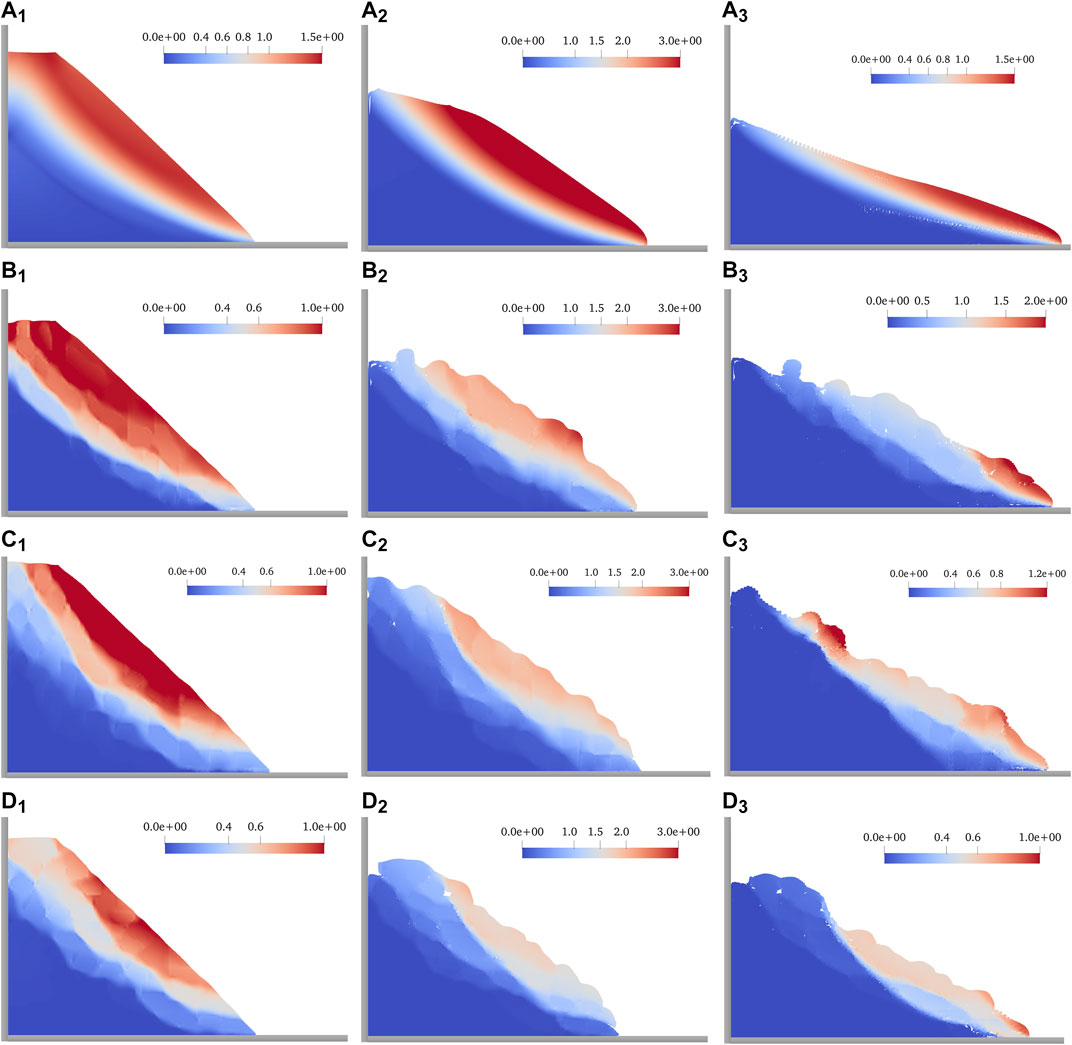
FIGURE 5. Rate cloud maps. (A₁) ∼(A₃) Rate (m/s) distribution of the homogeneous soil slope at 0.5, 1.6, and 3.5 s. (B₁) ∼(B₃) Rate (m/s) distribution of the SRM slope (arbitrary shapes stones) at 0.5, 2.0 and 3.5 s. (C₁) ∼(C₃) Rate (m/s) distribution of the SRM slope (round stones) at 0.5, 1.5, and 3.5 s. (D₁) ∼(D₃) Rate (m/s) distribution of the SRM slope (oval stones) at 0.5, 1.8, and 3.5 s.

From the velocity distribution of the four slopes, the homogeneous soil slope is uniform and continuous; the SRM slope shows layered characteristics, and their distribution patterns also show different features due to various stones. In terms of speed, the maximum speed of the four slopes is the same in the acceleration stage (0.5s). At the peak energy moment, the velocity of the homogeneous soil slope is the largest, exceeding 3 m/s, and the smallest is the SRM slope with oval stones. The maximum velocity distribution range of homogeneous soil slope is the widest, followed by the SRM slope with arbitrary stones, and the smallest is the SRM slope with oval stones. In the deceleration stage (3.5s), the SRM slope with arbitrary shape stones has the highest velocity, which reaches 2 m/s, but it is only distributed at the front of the sliding body, and the speed in other areas is less than 1 m/s.

The plastic zone

Figure 6 draws the plastic zone distribution of 1s, 5s, and their peak kinetic energy moments, respectively. The plastic zone of the homogeneous soil slope is continuous and smooth from start to end, and the plastic zone of soil around the main plastic zone decreases uniformly. SRM slopes contain multiple plastic zones interlaced with each other and show an obvious rock-around phenomenon; that is, the plastic zone is distributed around the hard block, and that is, the stone shape plays a key role in the distribution of the plastic zone.

FIGURE 6

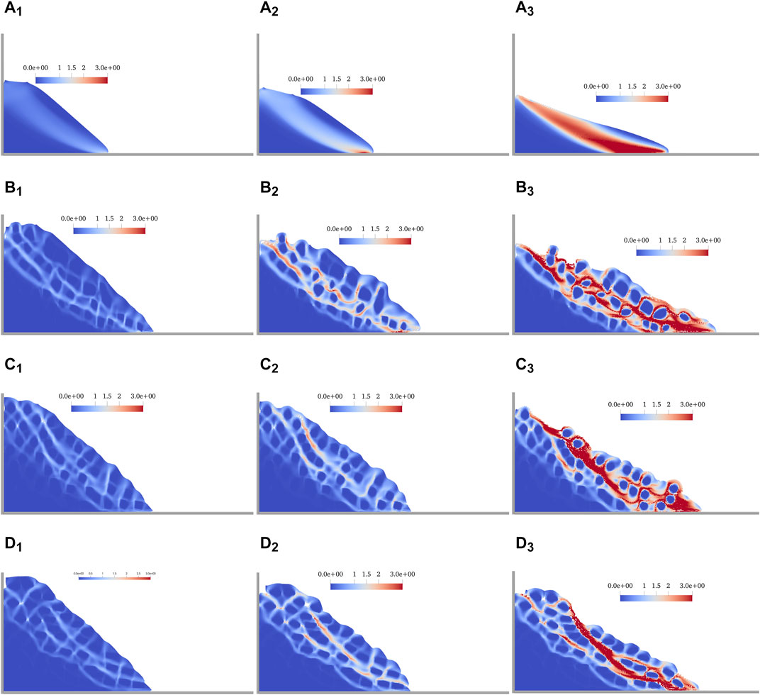
FIGURE 6. Variation of the plastic zone. (A₁) ∼ (A₃) Plastic zone distribution of the homogeneous soil slope at 1.0, 1.6, and 5.0 s. (B₁) ∼ (B₃) Plastic zone distribution of the SRM slope (arbitrary shape stones) at 1.0, 2.0, and 5.0 s. (C₁) ∼ (C₃) Plastic zone distribution of the SRM slope (round stones) at 1.0, 1.5, and 5.0 s. (D₁) ∼ (D₃) Plastic zone distribution of the SRM slope (oval stones) at 1.0, 1.8, and 5.0 s.

By comparing the plastic zone distribution of the SRM slopes, it can be found that the SRM slope with arbitrary shape stones is the most complex, and there is more soil entering the plastic yield state. In other words, the proportion of rock and soil still in a stable state is the smallest. The properties of the SRM at the bottom are as stable as those of bedrock. In summary, it can be concluded that under the same rock content, the larger volume and shape anisotropy of the rock is more beneficial to slope stability.

The displacement and final configuration

The accumulation configuration and maximum displacement of the slope after stability are shown in Figure 7, and Figure 8 shows the horizontal, vertical, and total displacements of four slopes after re-stabilization.

FIGURE 7

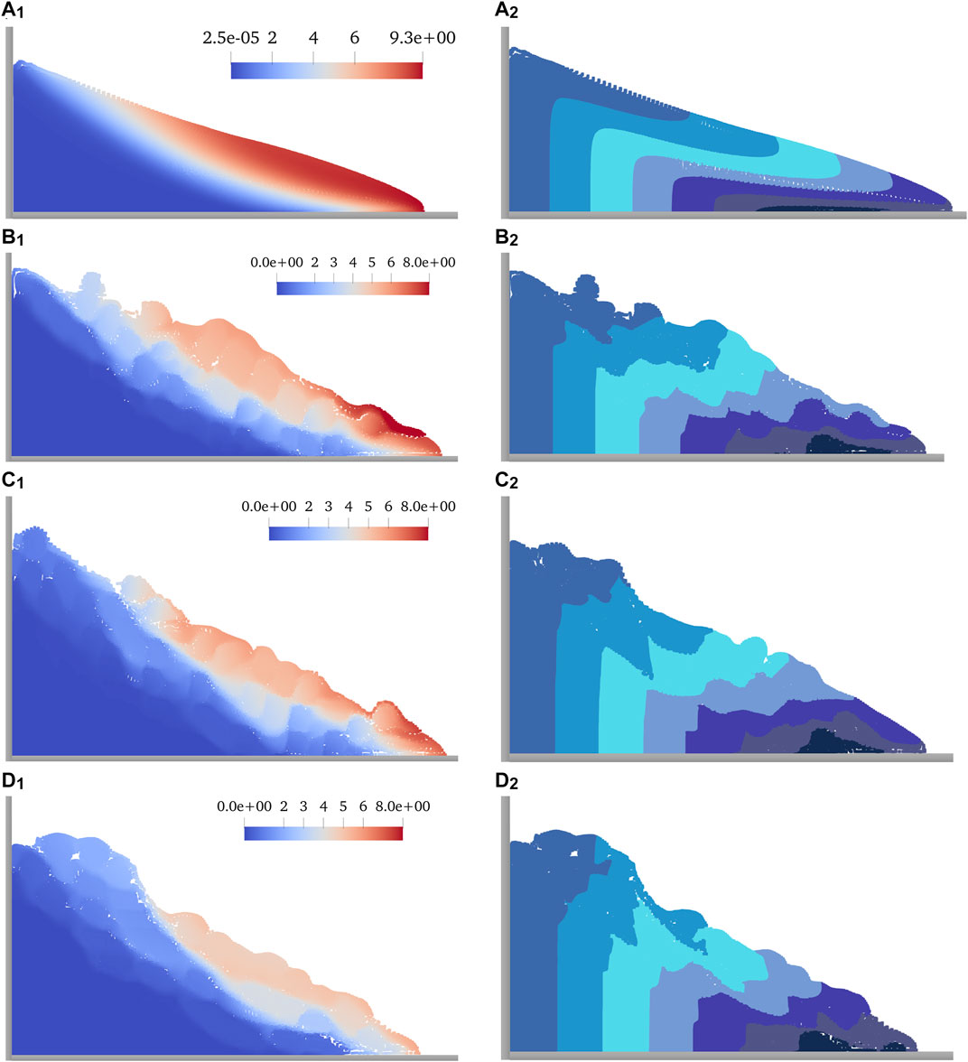
FIGURE 7. Displacement distribution and final configuration after the landslide. (A₁) Displacement (m) cloud map of the homogeneous soil slope at 10.0 s. (A₂) Final configuration of the homogeneous soil slope at 10.0 s. (B₁) Displacement (m) cloud map of the SRM slope (arbitrary shapes stones) at 10.0 s. (B₂) Final configuration of the SRM slope (arbitrary shapes stones) at 10.0 s. (C₁) Displacement (m) cloud map of the SRM slope (round stones) at 10.0 s. (C₂) Final configuration of the SRM slope (round stones) at 10.0 s. (D₁) Displacement (m) cloud map of the SRM slope (oval stones) rate at 10.0 s. (D₂) Final configuration of the SRM slope (oval stones) at 10.0 s.

FIGURE 8

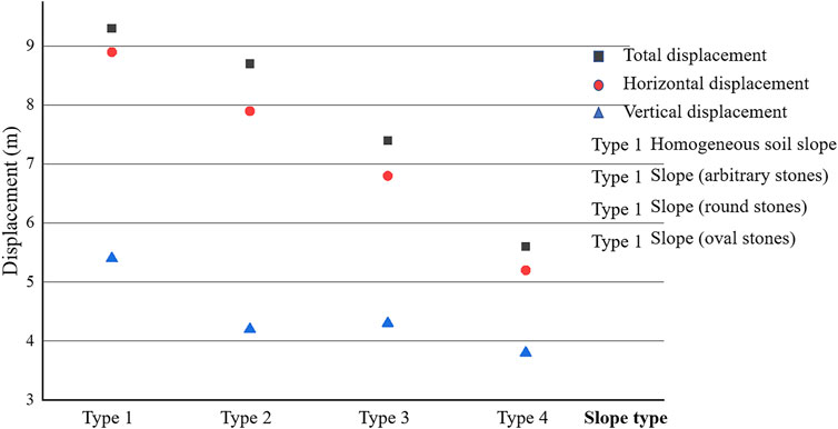
FIGURE 8. Total, horizontal, and vertical displacements after the slope is stabilized again.

According to Figure 8, the vertical displacement in the four slope models is very close to the total, indicating that the slope collapse mainly occurs in the vertical direction. The displacement of homogeneous soil slope is the largest, and the total, vertical, and horizontal displacement reach 9. 3, 8.9, and 5.4 m, respectively. Comparing the displacement of the SRM slopes, the SRM slope with oval stones has the minor displacement, followed by the SRM slope with round stones, and the SRM slope with arbitrary shape has the most significant displacement, about 8.7 m. Smaller stones can easily be carried by the soil and move together, while larger stones have large inertia, so it is difficult to change their motion state.

According to the final configuration and displacement distribution of each slope in Figure 7, compared with SRM slope with oval stones and SRM slope with round stones, the sliding area of the former is smaller, and the displacement of most areas is less than 2 m. Most of the bottom areas are stable without sliding. Areas with a more than 4 m displacement are concentrated in the front of the slope, mainly caused by the upper rock and soil collapse. By comparing their shapes, the SRM slopes with pebbles (i.e., C and D in Figure 7) are smoother than the SRM slope with stones of arbitrary shapes, second only to the homogeneous soil slope. The surface of SRM slope with arbitrary stones is not uniform, which indicates that the accumulation shape after SRM slope failure is closely related to the smoothness of stones.

Discussion

This article investigates the dynamic evolution of SRM slopes based on GIMP and compares it with that of homogeneous soil slopes, and investigates the influence of stone shape and size on the dynamic evolution of SRM slopes at the same stone content. However, there are some shortcomings in this research that need to be optimized, and they are discussed in detail as follows:

1) In actual engineering, the stone distribution of SRM slopes is highly random. Only four sets of simulations were performed in this article, which was limited by the arithmetic power of calculation when conducting the research. More and more randomly distributed stones should be set up for simulation and analysis in the future, and then a statistical rule can be derived. In addition, the factor of stone composition is not negligible under the same stone content, and the simulation analysis of SRM slopes with many different compositions may be able to obtain quantifiable results, which is self-evident for the guidance of practical engineering.

2) It is crucial to carry out model experiments and compare them with the results of numerical simulations. Subsequent collapse experiments should be carried out for homogeneous soils as well as SRM piles to record the pile morphology and rate at typical moments and the pile configuration when the collapse stops. Different SRM pile models are set up with different stones, and the location of each stone should be recorded to ensure that the numerical model is consistent with the physical model. It is guaranteed that each set of experiments is a single variable to improve the credibility of the experiments.

3) As SRM slopes mostly exist near the reservoir area, the influence of water on its stability is crucial, and the impact on the reservoir area after the slope collapse and slides into the reservoir area should also be considered. The subsequent work on fluid-solid coupling should be carried out based on the multiphase material point method, considering the water factor, conducting the targeted simulation, and improving numerical experiments.

Conclusion

In this article, the complex engineering problem of the SRM slope is studied, mainly considering two factors: the size and the shape of the stones. First, four slope models are established according to the engineering practice, and then the failure process is simulated and analyzed by GIMP. The conclusions are as follows:

1) For slopes with the same geometric size, the duration of their failure is the same, regardless of whether they contain stones; the homogeneous slope has more tremendous kinetic energy during a landslide, and it slides out farther. The order of kinetic energy of SRM slope is: SRM slope with arbitrary stones, SRM slope with round stones, SRM slope with oval stones. The reason is that the small stones will be wrapped in the soil and slide together, and the contribution of oval pebbles with large-scale differences in an orthogonal direction to the stability of the slope is better than that of round pebbles.

2) The plastic zone of homogeneous slope failure is a penetrating strip, while the plastic zone of SRM slope is interlaced with multiple plastic zones, showing an apparent rock-surrounding phenomenon. Under the condition of the same stone content, the soil entering the plastic zone in the SRM slope with large stones is smaller than that with little stones. The soil entering the plastic yield in SRM slope with oval stones with large shapes anisotropy is the least, and there are many rocks and soil at the bottom without any plastic deformation.

3) The accumulation form after the failure of the slope is closely related to whether there are stones in it. Whether the stones are smooth will also affect the shape of the accumulation body. Any shape of stones will lead to an uneven slope surface, while the slope containing smooth pebbles is relatively smooth.

Data availability statement

The original contributions presented in the study are included in the article/Supplementary Material; further inquiries can be directed to the corresponding author.

Author contributions

XL: resources, data curation, and project; P-FX: software; YZ: writing—original draft preparation; JL and L-JW: resources, data curation, and project; K-YH: validation and investigation; TJ: editing.

Funding

This work was financially supported by the National Natural Science Foundation of China (No. 52108304) and the Open Fund of Chongqing Key Laboratory of Energy Engineering Mechanics and Disaster Prevention and Mitigation (No. EEMDPM2021101).

Conflict of interest

JL and L-JW were employed by the company Chongqing Water Conservancy and Electric Power Survey and Design Institute Co., Ltd.

The remaining authors declare that the research was conducted in the absence of any commercial or financial relationships that could be construed as a potential conflict of interest.

Publisher’s note

All claims expressed in this article are solely those of the authors and do not necessarily represent those of their affiliated organizations, or those of the publisher, the editors, and the reviewers. Any product that may be evaluated in this article, or claim that may be made by its manufacturer, is not guaranteed or endorsed by the publisher.

References

Andersen, S., and Andersen, L. (2010). Modelling of landslides with the material-point method. Comput. Geosci. 14 (1), 137–147. doi:10.1007/s10596-009-9137-y

CrossRef Full Text | Google Scholar

Bardenhagen, S. G., and Kober, E. M. (2004). The generalized interpolation material point method. CMES - Comput. Model. Eng. Sci. 5 (6), 477–495. doi:10.3970/cmes.2004.005.477

CrossRef Full Text | Google Scholar

Cen, D., Huang, D., and Ren, F. (2017). Shear deformation and strength of the interphase between the soil-rock mixture and the benched bedrock slope surface. Acta Geotech. 12 (2), 391–413. doi:10.1007/s11440-016-0468-2

CrossRef Full Text | Google Scholar

Chen, Z., and Brannon, R. (2002). An evaluation of the material point method. Albuquerque, New Mexico, United States: Sandia National Laboratories, 46. doi:10.2172/793336February

CrossRef Full Text | Google Scholar

Cui, S., Pei, X., Jiang, Y., Wang, G., Fan, X., Yang, Q., et al. (2021). Liquefaction within a bedding fault: Understanding the initiation and movement of the daguangbao landslide triggered by the 2008 wenchuan earthquake (Ms=8.0). Eng. Geol. 295, 106455. doi:10.1016/j.enggeo.2021.106455

CrossRef Full Text | Google Scholar

Cui, X. X., Zhang, X., Sze, K. Y., and Zhou, X. (2013). An alternating finite difference material point method for numerical simulation of high explosive explosion problems. CMES - Comput. Model. Eng. Sci. 92 (5), 507–538. doi:10.3970/cmes.2013.092.507

CrossRef Full Text | Google Scholar

de Vaucorbeil, A., Nguyen, V. P., Sinaie, S., and Wu, J. Y. (2020). “Material point method after 25 Years: Theory, implementation, and applications,” in Advances in applied mechanics (Amsterdam, Netherlands: Elsevier), 53, 185–398.

CrossRef Full Text | Google Scholar

Guide, A. P. (2019). The material point method for geotechnical engineering: A practical Guide. Boca Raton: CRC Press, 3–22.

Google Scholar

He, Y., and Kusiak, A. (2018). Performance assessment of wind turbines: Data-derived quantitative metrics. IEEE Trans. Sustain. Energy 9 (1), 65–73. doi:10.1109/TSTE.2017.2715061

CrossRef Full Text | Google Scholar

Jiang, Y., Li, M., Jiang, C., and Alonso-Marroquin, F. (2020). A hybrid material-point spheropolygon-element method for solid and granular material interaction. Int. J. Numer. Methods Eng. 121 (14), 3021–3047. doi:10.1002/nme.6345

CrossRef Full Text | Google Scholar

Li, H., Deng, J., Feng, P., Pu, C., Arachchige, D. D. K., Cheng, Q., et al. (2021a). Short-term nacelle orientation forecasting using bilinear transformation and ICEEMDAN framework. Front. Energy Res. 9, 780928. doi:10.3389/fenrg.2021.780928

CrossRef Full Text | Google Scholar

Li, H., Deng, J., Yuan, S., Feng, P., and Arachchige, D. D. K. (2021b). Monitoring and identifying wind turbine generator bearing faults using deep belief network and EWMA control charts. Front. Energy Res. 9, 799039. doi:10.3389/fenrg.2021.799039

CrossRef Full Text | Google Scholar

Li, H., He, Y., Xu, Q., Deng, J., Li, W., Wei, Y., et al. (2022). Detection and segmentation of loess landslides via satellite images: A two-phase framework. Landslides 19 (3), 673–686. doi:10.1007/s10346-021-01789-0

CrossRef Full Text | Google Scholar

Liu, P., Liu, Y., and Zhang, X. (2015). Improved shielding structure with double honeycomb cores for hyper-velocity impact. Mech. Res. Commun. 69, 34–39. doi:10.1016/j.mechrescom.2015.06.003

CrossRef Full Text | Google Scholar

Liu, P., Liu, Y., and Zhang, X. (2016). Simulation of hyper-velocity impact on double honeycomb sandwich panel and its staggered improvement with internal-structure model. Int. J. Mech. Mat. Des. 12 (2), 241–254. doi:10.1007/s10999-015-9300-7

CrossRef Full Text | Google Scholar

Liu, X., Wang, Y., and Li, D. Q. (20182019). Investigation of slope failure mode evolution during large deformation in spatially variable soils by random limit equilibrium and material point methods. Comput. Geotechnics 111, 301–312. doi:10.1016/j.compgeo.2019.03.022

CrossRef Full Text | Google Scholar

Mast, C. M. (2013). Modeling landslide-induced flow interactions with structures using the material point method. Washington: University of Washington, 263.

Google Scholar

Nairn, J. A., and Guo, Y. J. (2005). Material point method calculations with explicit cracks, fracture parameters, and crack propagation, 11th International Conference on Fracture 2005, Turin, March 20–March 25, 2005, 2, 6. ICF11, 1192–1197.

Google Scholar

Napoli, M. L., Barbero, M., and Scavia, C. (2021). Effects of block shape and inclination on the stability of melange bimrocks. Bull. Eng. Geol. Environ. 80 (10), 7457–7466. doi:10.1007/s10064-021-02419-8

CrossRef Full Text | Google Scholar

Springman, S. M., Jommi, C., and Teysseire, P. (2003). Instabilities on moraine slopes induced by loss of suction: A case history. Geotechnique 53 (1), 3–10. doi:10.1680/geot.2003.53.1.3

CrossRef Full Text | Google Scholar

Sulsky, D., Chen, Z., and Schreyer, H. L. (1994). A particle method for history-dependent materials. Comput. Methods Appl. Mech. Eng. 118 (1–2), 179–196. doi:10.1016/0045-7825(94)90112-0

CrossRef Full Text | Google Scholar

Tang, M., Xu, Q., and Huang, R. (2015). Site monitoring of suction and temporary pore water pressure in an ancient landslide in the three Gorges reservoir area, China. Environ. Earth Sci. 73 (9), 5601–5609. doi:10.1007/s12665-014-3814-4

CrossRef Full Text | Google Scholar

Wang, B., Vardon, P. J., Hicks, M. A., and Chen, Z. (2016). Development of an implicit material point method for geotechnical applications. Comput. Geotechnics 71, 159–167. doi:10.1016/j.compgeo.2015.08.008

CrossRef Full Text | Google Scholar

Yang, Y., Sun, G., Zheng, H., and Qi, Y. (2019). Investigation of the sequential excavation of a soil-rock-mixture slope using the numerical manifold method. Eng. Geol. 256, 93–109. doi:10.1016/j.enggeo.2019.05.005

CrossRef Full Text | Google Scholar

Ye, Z., Zhang, X., Zheng, G., and Jia, G. (2018). A material point method model and ballistic limit equation for hyper velocity impact of multi-layer fabric coated aluminum plate. Int. J. Mech. Mat. Des. 14 (4), 511–526. doi:10.1007/s10999-017-9387-0

CrossRef Full Text | Google Scholar

Yilmaz, I., Marschalko, M., Bednarik, M., Kaynar, O., and Fojtova, L. (2012). Neural computing models for prediction of permeability coefficient of coarse-grained soils. Neural comput. Appl. 21 (5), 957–968. doi:10.1007/s00521-011-0535-4

CrossRef Full Text | Google Scholar

Ying, C., Zhang, K., Wang, Z. N., Siddiqua, S., Makeen, G. M. H., Wang, L., et al. (2021). Analysis of the run-out processes of the xinlu village landslide using the generalized interpolation material point method. Landslides 18 (4), 1519–1529. doi:10.1007/s10346-020-01581-6

CrossRef Full Text | Google Scholar

Yue, Z. Q., and Morin, I. (1996). Digital image processing for aggregate orientation in asphalt concrete mixtures. Can. J. Civ. Eng. 23 (2), 480–489. doi:10.1139/l96-052

CrossRef Full Text | Google Scholar

Zabala, F., and Alonso, E. E. (2012). “The material point method and the analysis of dams and dam failures,” in Innovative numerical modelling in geomechanics (Boca Raton, Florida, United States: CRC Press), 171–177.

Google Scholar

Zhang, D. Z., and Jayaraman, B. (2013). Equations and closure models for material pulverization and debris flow. Int. J. Multiph. Flow 56, 149–159. doi:10.1016/j.ijmultiphaseflow.2013.06.001

CrossRef Full Text | Google Scholar

Zhang, Z. L., Xu, W. J., Xia, W., and Zhang, H. Y. (2016). Large-scale in-situ test for mechanical characterization of soil-rock mixture used in an embankment dam. Int. J. Rock Mech. Min. Sci. 86, 317–322. doi:10.1016/j.ijrmms.2015.04.001

CrossRef Full Text | Google Scholar

Zhao, X., Liang, D., and Martinelli, M. (2017). MPM simulations of dam-break floods. J. Hydrodyn. 29 (3), 397–404. doi:10.1016/S1001-6058(16)60749-7

CrossRef Full Text | Google Scholar

Zhou, J., Wei, J., Yang, T., Zhang, P., Liu, F., Chen, J., et al. (2021). Seepage channel development in the crown pillar: Insights from induced microseismicity. Int. J. Rock Mech. Min. Sci. 145, 104851. doi:10.1016/j.ijrmms.2021.104851

CrossRef Full Text | Google Scholar