Positive mass budgets of high-altitude and debris-covered fragmented tributary glaciers in Gangotri Glacier System, Himalaya

1 Introduction

The Himalayan region—The Third Pole—is the source of several perennial river systems in South Asia including the Indus, Ganga, and the Brahmaputra, and provides a steady supply of freshwater for over a billion people, which is used for drinking, hydropower generation, agriculture, sanitation, and other purposes (Azam et al., 2021). With an area of 42,525 km² (including the Karakoram Range), the Himalaya implies the largest concentration of glaciers outside the polar regions (Nuimura et al., 2015). Emerging evidence of continuous, accelerated, and spatially heterogeneous rates of glacier mass loss in the Himalaya since the mid-nineteenth century raised the scientific community’s attention to the regional differences in climatic conditions and the paucity of in situ observations in the Himalaya (Brun et al., 2017; Sakai and Fujita, 2017; Azam et al., 2018; Bolch et al., 2019; Maurer et al., 2019; Shean et al., 2020). In the west of the Himalaya, Karakoram glaciers have demonstrated an exceptional worldwide case of balanced or positive mass budgets, termed the “Karakoram Anomaly” (Hewitt, 2005; Kääb et al., 2012; Gardelle et al., 2013).

In situ glacier-wide mass balance (MB) monitoring of glaciers provides an understanding of the quick response of the glaciers to local meteorological conditions (Oerlemans, 2001). Several in situ glaciological studies are being conducted over the different basins of the Himalaya (Dobhal et al., 2013; Mandal et al., 2020; Wagnon et al., 2021; Stumm et al., 2021) but these observations are still sparser compared to the other glacierized regions of the world (Zemp et al., 2015; Azam et al., 2018). Due to the harsh climatic conditions, low oxygen level, and steep terrain of the Himalaya, the in situ MBs have only been observed for a short period and on a few small glaciers (Azam et al., 2018). However, as satellite missions and remote sensing methods progressed, it has become possible to work at a regional scale using geodetic method (Bolch et al., 2019; Shean et al., 2020), but the uncertainty associated with the sensors and inability to estimate the interannual and seasonal variations of glacier MB limit its applicability to understand the glacier-climate relationship (Vincent et al., 2018).

Due to the scarcity of in situ MB observations in the Himalaya, modelling approaches have been used to understand the MB variability with climatic parameters (Azam et al., 2018). These models range from simple temperature-index (T-index) to complex surface energy balance (SEB) models (Hock and Holmgren, 2005; Pellicciotti et al., 2005; Srivastava and Azam, 2022a). The SEB model applications, required to understand the impact of different climate variables on glacier health, are limited in the Himalaya because of the need of extensive input data (Azam et al., 2014a; Mandal et al., 2022; Oulkar et al., 2022). On the other hand, the T-index models require minimal data, often only the temperature (Hock, 2003). The good performance of T-index models compared to SEB models is attributed to the fact that many components of energy balance, such as long wave radiation, sensible heat flux, are strongly correlated with temperature (Ohmura, 2001). Therefore, despite the simple computation of the T-index models, they have been applied widely to the Himalayan glaciers to reconstruct the long-term glacier MBs (Azam et al., 2014b; Shea et al., 2015; Litt et al., 2019; Pratap et al., 2019; Srivastava and Azam, 2022b).

Glacier MB reconstructions using the simple T-index models have been carried out in different parts of the Himalaya, especially on the glaciers where some in situ data is available (Azam et al., 2018). A short-term study on the Chandra Basin (8 glaciers from whole basin, area ranging from 2 to 78 km²) showed the mean MB of –0.71 ± 0.34 m w. e. a^‒ˡ over 2000–2009 (Tawde et al., 2016). Another study modelled the mean MB of –0.68 m w. e. a^‒ˡ over 1985–2014 on four selected glaciers (Naradu, Shaune Garang, Gor-Garang and Gara glaciers) in the Baspa Basin (Gaddam et al., 2017). The MB of Naimona’nyi Glacier (14.4 km²) was reconstructed as –0.40 ± 0.17 m w. e. a^‒ˡ over 1974–2014 (Zhao et al., 2016). Patsio Glacier (Bhaga Basin having area of 2.5 km²) showed the modelled mean mass loss of –0.10 ± 0.10 m w. e. a^‒ˡ over the period 1993–2018 (Kumar et al., 2021). The longest reconstructed MB series is available from Chhota Shigri and Dokriani Bamak glaciers with moderate mass wastages of –0.12 ± 0.28 m w. e. a^‒ˡ and –0.09 ± 0.35 m w. e. a^‒ˡ over the last 7 decades (1950–2020) (Srivastava et al., 2022). These recent applications suggest that the T-index models can reconstruct the mass balances, especially in data-scarce region like the Himalaya.

Further, the in situ observations, as well as the model applications, are often available from small glaciers, and the large glaciers have not been investigated in the Himalaya. The presence of ice cliffs and supra-glacial lakes on the debris-covered surface of the large Himalayan glaciers is another challenge that cannot be included in T-Index model due to extensive data requirement to compute melt over these surfaces.

For the present study, we have selected Gangotri Glacier System (Gangotri, Chaturangi, Raktavaran and Meru glaciers) and reconstructed its annual and seasonal MBs since 1979 using a simple T-Index model combined with an accumulation model. The Gangotri Glacier System is selected because it has one of the biggest glaciers (Gangotri Glacier) in India and has already been studied using the geodetic approaches (Bhattacharya et al., 2016; Bhushan et al., 2017). The major objectives of this study are 1) to test T-index model applicability for a large, highly-debris covered glacier with ice cliffs and supra-glacial lakes, 2) to model the long-term annual and seasonal MB series for all glaciers of the Gangotri Glacier System and 3) to understand the modelled MB sensitivity to input parameters and climate data.

2 Study area and climatic conditions

2.1 Study area

The Gangotri Glacier System (30.72°–31.02° N, 78.99°–79.29° E) is the largest glacier system in the Bhagirathi Basin, located in the Garhwal range of the central Himalaya in the Uttarakhand state of India. It is having four glaciers namely: Gangotri, Chaturangi, Raktavaran and Meru (Figure 1; GSI, 2009). The system originates from the Chaukhamba massif ∼7,000 m a.s.l, flows from SE to NW within the granitic terrain, and terminates at ∼4,000 m a.s.l. with a total glacierized area of ∼252 km² (Figure 1). Gangotri Glacier System shapefile was extracted from the GAMDAM Glacier Inventory, in which the glacier outlines were delineated manually using high resolution Google earth images, DEM, and Landsat ETM data from 1999 to 2003. (Nuimura et al., 2015). Gangotri Glacier System also has its religious importance, and its snout is called Gaumukh (mouth of a cow). The Bhagirathi River flows from the Gaumukh to Devprayag, where it joins the Alaknanda River to form the Ganga River.

FIGURE 1

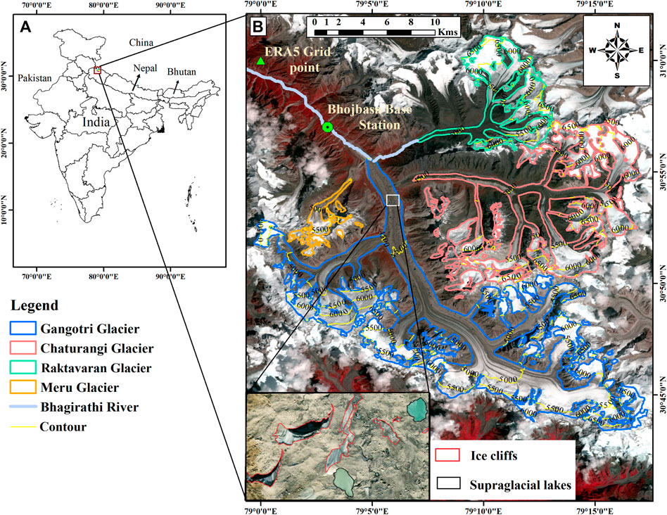
FIGURE 1. (A) Panel shows the location of the Gangotri Glacier System, India. (B) Panel shows all four glaciers Gangotri (blue), Chaturangi (red), Raktavaran (green) and Meru (yellow) on Landsat eight image of 13th September 2017, and the inset (left bottom of B) shows the enlarged view of ice cliffs (red outlines) and supra-glacial lakes (black outlines) on the surface of Gangotri Glacier.

The Gangotri Glacier System is surrounded by mystic peaks (ranging from 6,000–7,000 m a.s.l.). The main trunk of Gangotri Glacier is ∼32 km long and 1–3 km wide, with Meru Glacier on the left and Chaturangi and Raktavaran glaciers on the right (Figure 1). Historical evidences indicate that Meru, Chaturangi and Raktavaran glaciers were tributary glaciers of the main Gangotri Glacier and got fragmented in the past (GSI, 2004). The topographical details of all glaciers in the Gangotri Glacier System are given in Table 1. All four glaciers of the Gangotri Glacier System are heavily debris-covered (Figure 1) and have around 20% debris cover area, found increasing with an increasing rate over recent decades (Bhattacharya et al., 2016). Gangotri Glacier has the highest debris cover (24% of its total area) and has numerous ice cliffs and glacial lakes on its lower ablation area (inset of Figure 1) that are expected to act as melting hotspots hence amplify the local melting (Brun et al., 2018; King et al., 2019; Shugar et al., 2020). Debris covers, ice cliffs and supraglacial lakes were manually delineated on the Google earth image of 6 October 2019, near the end of the melting season for clear visibility of all these features. The climatic condition of the Gangotri Glacier System is influenced regionally by the Indian summer Monsoon (ISM) and Indian winter Monsoon (IWM) (Dimri et al., 2016; Kotlia et al., 2018).

TABLE 1

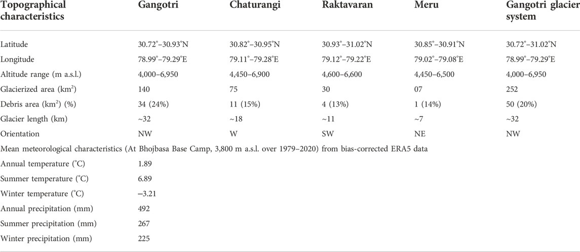
TABLE 1. Topographical and meteorological characteristics of the Gangotri Glacier System.

2.2 Data, bias correction and climatic conditions

Daily reanalysis temperature and precipitation data available at 0.25° X 0.25° resolution from ERA5 (https://cds.climate.copernicus.eu) were used to determine the annual and seasonal MBs of all glaciers in the Gangotri Glacier System since 1979. The ERA5 reanalysis temperature and precipitation data were downloaded at the nearest grid point (∼8 km) to the Bhojbasa Base Camp (3,800 m a.s.l.) (Figure 1).

The mean monthly temperature data from May 2006 to April 2007 from an Automatic Weather Station (AWS) at Bhojbasa Base Camp (Agrawal et al., 2018) was used for bias correction of raw ERA5 temperature data. Raw ERA5 mean monthly temperature exhibited a high correlation with AWS temperature (Figure 2A). In situ precipitation data was available only for the summer months (May-October) over 2000–2003 (Singh et al., 2006) and utilised for bias correction of the raw ERA5 precipitation data. ERA5 precipitation data also showed high correlation but high overestimation (Figure 2B) with the available mean monthly precipitation data. The multiplicative monthly bias-correction factors, developed from the linear regression equation between the mean monthly ERA5 and in situ temperature and precipitation data, were applied to bias-correct the daily data. The multiplicative factors were 1.12 and 0.42 for the temperature and precipitation data, respectively (Figures 2A,B).

FIGURE 2

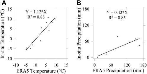
FIGURE 2. (A) Panel shows the regression fit between in situ temperature and reanalysed ERA5 temperature over 2006–2007 (B) Panel shows the regression fit between in situ precipitation and reanalysed ERA5 precipitation over 2000–2003.

The long-term in situ meteorological data is not available hence in this study we used the bias-corrected ERA5 temperature and precipitation for the period 1979–2020 to understand the local temperature and precipitation distribution over the year. The bias-corrected ERA5 annual mean temperature at the Bhojbasa Base Camp was 1.89 °C, with the highest and lowest annual mean temperatures of 3.26°C and 0.62°C for 2016 and 1997, respectively (Figure 3A). The mean temperatures in the summer (May–October) and winter (November–April) months were 6.89°C and –3.21°C, respectively. July was the hottest month with a mean temperature of 10.1°C and January was the coldest with a minimum temperature of –6.74°C over 1979–2020 (Figure 3B). The bias-corrected ERA5 mean annual precipitation was 492 mm, with 54% occurring during the summer season and 46% during the winter season, indicating that Gangotri Glacier System receives nearly equal precipitations in both the seasons (Figure 3B).

FIGURE 3

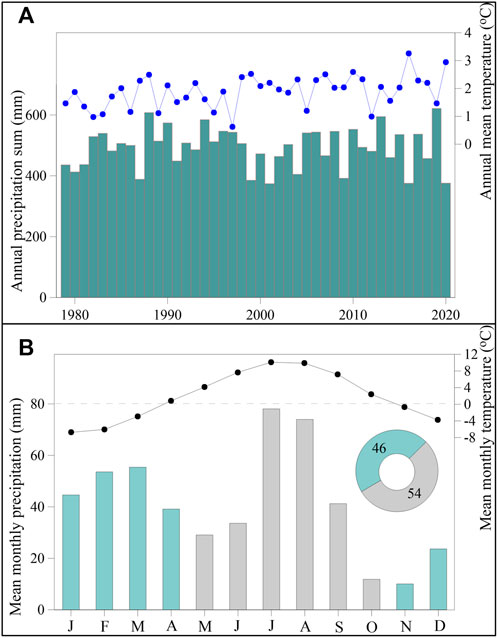
FIGURE 3. (A) Bias-corrected annual mean temperature (blue dots) and annual precipitation sums (green bars) over 1979–2020 and (B) bias-corrected mean monthly precipitation and temperature patterns at Bhojbasa Base Camp (black dots represent the temperature, blue-green bars represent the winter precipitation, and the grey bars represent the summer precipitation) and the pie chart inset shows the percent of seasonal precipitation contribution.

Gangotri Glacier System is located on the leeward side of the mountain range. The mean annual precipitation at Bhojbasa Base Camp (492 mm) is only 30% of that of Dokriani Bamak Glacier Base Camp (1,616 mm), a glacier that is located on the orographic front in the same range around 30 km SW of Gangotri Glacier (Azam and Srivastava, 2020). Because high-altitude orographic forcing influences the amount of precipitation (Bhaskaran et al., 1996; Dimri et al., 2013), the ISM reach over the Gangotri Glacier System is quite poor. Dokriani Bamak Glacier receives its 77% of annual precipitation from the summer months and is thought to be a summer-accumulation type glacier (Srivastava and Azam, 2022a), while Gangotri Glacier System receives an almost equal amount of summer and winter precipitations (Table 1) that makes it difficult to say whether it is summer- or winter-accumulation type glacier system. This comparison clearly demonstrates that different types of glaciers can co-exist in the same range due to the complex topography that gives rise to the local microclimate.

3 Methodology

3.1 Mass balance model

The annual and seasonal MBs of all glaciers in the Gangotri Glacier system are reconstructed by applying a T-index model together with an accumulation model that has been applied in several previous studies for MB reconstructions in the Himalaya (Azam et al., 2014b; Srivastava and Azam, 2022a). The model is forced with the bias-corrected ERA5 daily precipitation and temperature data since 1979. The model runs at a daily time scale and estimates the daily accumulation and ablation for each altitudinal range of 50-m for a full hydrological year, from November 1 to October 31.

The daily precipitation and temperature are extrapolated to each 50-m altitudinal range by applying the altitudinal precipitation gradient (P_g) and temperature lapse rates (LRs), respectively.

$P=P_i+P_{g}X\mathit{\Delta }H(1)$

Where P is the calculated precipitation at different altitudinal bands, P_i is the precipitation at base camp, ΔH is the altitudinal difference between Bhojbasa Base Camp and the corresponding altitudinal band (m) and P_g is the precipitation gradient in % precipitation change per 1,000 m altitude. P_g has been used to extrapolate the precipitation at a daily scale because our model runs at a daily scale.

$T=T_i–LRX\mathit{\Delta }H(2)$

Where T is the calculated temperature at different altitudinal bands, T_i is the temperature at Bhojbasa Base Camp, ΔH is the altitudinal difference between base camp and corresponding altitudinal band (m) and LR is the monthly lapse rate.

The daily accumulation (A) is estimated by using the threshold temperature for snow/rain (T_P) and the daily ablation (M) is estimated by using the threshold temperature for melt (T_M). Accumulation of snow is taken place when T < T_P, and if T > T_P all the snow is melted.

The daily accumulation A (mm w. e. d⁻¹) at each altitudinal range is computed by:

$A=\{\begin{array}{c}P:T\le T_P\\ 0:T>T_P\end{array}(3)$

Where P and T are daily precipitation (mm) and temperature (°C) respectively extrapolated at each altitudinal range and T_P is the threshold temperature (°C) for snow-rain.

Ablation (M) is taken place when T > T_M, otherwise it is computed to be zero. During melting, first, the accumulated snow is melted out and then ice is started melting depending on the surface condition whether it is debris cover or clean ice.

The daily ablation M (mm w. e. d⁻¹) at each altitudinal range is computed by:

$M=\{\begin{array}{c}DD{F}_{S/I/D}\cdot \left(T-T_M\right):T>T_M\\ 0:T\le T_M\end{array}(4)$

where, DDF_S/I/D denotes the degree-day factor (mm d⁻¹°C⁻¹) for snow (S), ice (I) and debris-covered ice (D) surfaces, and T is extrapolated daily air temperature (°C) at each altitudinal range. In addition, DDF_I was also employed for ablation on the thick debris-covered surface of Gangotri Glacier which has numerous ice cliffs and supra-glacial lakes (Section 5.2).

Daily mean altitudinal MB (b_i) at each 50-m altitudinal range is calculated using daily M and daily A (from Eqs. 3, 4):

$b_i=A–M(5)$

Glacier-wide MB (B_a) is calculated as:

$B_a=\mathrm{\Sigma }{b}_i\left(a_i/A\right)(6)$

where b_i is the altitudinal MB at each altitude, a_i is the area for each altitude, and A is the total glacier area.

3.2 Model parameters

The temperature is the most important variable controlling the distribution of snow/rain on the surface and the melting of snow and ice surface in T-index glacier MB modelling (Shea et al., 2015). The in situ DDF for snow, ice, and debris-cover are not available for Gangotri Glacier System and were taken as 6.1, 7.7 and 4.8 mm d⁻¹°C⁻¹, respectively, which were calculated (Azam and Srivastava, 2020) based on the previous in situ observations from different studies on the Dokriani Bamak Glacier located ∼30 km west of Gangotri Glacier System (Singh et al., 2000; Pratap et al., 2015). The T_P is taken as 0.7°C from (Jennings et al., 2018), which corresponds to 70–80% relative humidity ranges for Gangotri Glacier System. The temperature is extrapolated at different altitudinal ranges using the monthly LRs developed on the Dokriani Bamak Glacier catchment (Azam and Srivastava, 2020). Monthly LRs vary with the highest mean monthly LR (6.94°C km⁻¹) in May and the lowest mean monthly LR (5.42°C km⁻¹) in August. T_M and P_g are used to calibrate the model (Section 3.3). All the model parameters are listed in Table 2.

TABLE 2

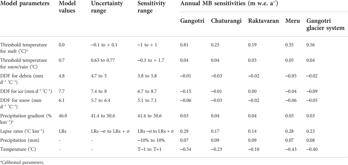
TABLE 2. List of model parameters and range of parameters used for uncertainties and sensitivities of MB.

3.3 Model calibration

The precipitation distribution in the complex Himalayan terrain is poorly known because of very limited in situ observations (Azam et al., 2021), hence the suitable selection of P_g for precipitation distribution on the glaciers is always challenging in the mountainous region (Immerzeel et al., 2015; Bolch et al., 2019). Another critical parameter is T_M, for which the MB models are very sensitive (Engelhardt et al., 2017; Azam and Srivastava, 2020). Further, studies suggest that sometimes melting does not even happen at an air temperature of >0°C (Kuhn, 1987; Hock, 2003) however, some T-index model studies suggest that the calibrated T_M can be negative at the daily time step (van den Broeke et al., 2010; Engelhardt et al., 2017; Azam and Srivastava, 2020). So, P_g and T_M are chosen as the calibrating parameters and varied to fit the model output with the observed geodetic MB data. The T_M and P_g were altered between ‒5 and 5°C, and 0% km⁻¹ and 100% km⁻¹, respectively. The Monte Carlo simulations (10,000 runs) were performed for the model calibration while minimizing the root mean square errors (RMSE) between the modelled and available geodetic MB (‒0.29 ± 0.19 m w. e. a^‒ˡ) over 2006–2014 for Gangotri Glacier System (Bhattacharya et al., 2016). The geodetic MBs for different glaciers in Gangotri Glacier System are not available separately hence the geodetic MB available for the whole Gangotri Glacier System has been used for model calibration. T_M of 0°C and P_g of 46% km⁻¹ showed the least RMSE of 0.08, corresponding to a mass wastage of ‒0.27 ± 0.25 m w. e. a^‒ˡ over 2006–2014 for the Gangotri Glacier System. Same calibrated parameters were applied separately on Gangotri Glacier and other fragmented tributary glaciers of the Gangotri Glacier System to simulate the corresponding annual and seasonal MBs.

3.4 Model validation

The model is validated against the manually delineated snow line altitudes (SLAs) derived from the Landsat satellite images with the modelled SLAs. The modelled SLAs are independently derived with the calibrated parameters at the 5-m altitudinal range. The uncertainty in modelled SLAs was assumed to be equal to 10 m as the model ran at a 5-m altitudinal range. Total of 19 SLAs are derived from Landsat satellite images on cloud-free days from 1989 to 2019. The modelled and satellite-derived SLAs showed a good agreement but high RMSE (r = 0.69 and RMSE = 208 m, Figure 4). The possible reasons for mismatch could be due to an error in the manual delineation of SLAs caused by the presence of shadows in the satellite images as well as the coarser resolution of the images. Additionally, the assumption of a single SLA for the entire glacier in the model estimation could be the cause of the larger RMSE, as SLA may have several altitudes in different parts of the glacier due to various aspects and local topography (Racoviteanu et al., 2019).

FIGURE 4

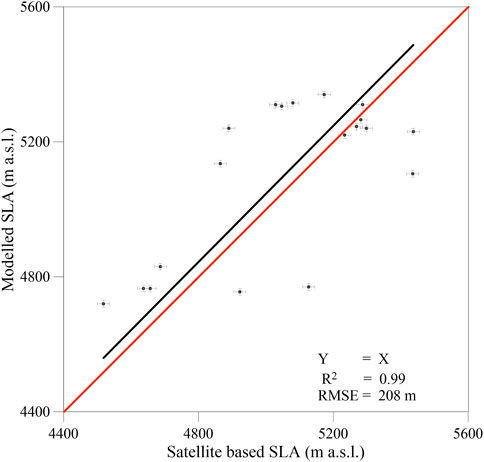
FIGURE 4. Validation of modelled snow line altitudes (SLAs) with satellite-derived SLAs for selected 19 days between 1989 and 2019. Vertical and horizontal bars show the uncertainties in modelled SLAs and satellite-derived SLAs, respectively.

The uncertainty in SLA is estimated using the similar method as followed in (Racoviteanu et al., 2019), in which the accuracy of the digital elevation model (DEM) and buffer size are used for the partition of surface and SLA extraction, respectively and the uncertainty in the snow and ice area estimates are also considered. We used Cartosat-1 DEM for surface partition and Landsat satellite images for snow and ice area estimation (Racoviteanu et al., 2019). The SLA uncertainty as $\pm$ 18.03 m was calculated with the formula:

${\varepsilon }_{SLA}=\sqrt{{\varepsilon }_{DEM}^2+{\varepsilon }_{SNOWLINE}^2}(7)$

Where ɛ_DEM is the vertical error of the Cartosat-1 DEM as $\pm$ 9.6 m (Singh et al., 2013) and ɛ_SNOWLINE is half the pixel size of the Landsat image as $\pm$ 15 m (Racoviteanu et al., 2019).

3.5 Uncertainty estimation

Each model parameter is altered one by one, within a 10% range of its calibrated value (except for parameters that are constrained using in situ data, and uncertainty range is known and used) to estimate the parametric uncertainty on the model outputs, while the other parameters are maintained constant (Anslow et al., 2008; Heynen et al., 2013; Ragettli et al., 2013). The plausible ranges of model parameters are given in Table 2. The overall model uncertainties for the modelled MBs were estimated using error propagation law and found as ± 0.31, ±0.17, ±0.15, ±0.29, ±0.25 m w. e. a^‒ˡ for Gangotri Glacier, Chaturangi Glacier, Raktavaran Glacier, Meru Glacier and Gangotri Glacier System, respectively.

The areal extent and hypsometry of the study area have been kept fixed for modelling the MBs in the present study. The areal shrinkage on Gangotri Glacier between 1962 and 2006 was only 6% of its area in 1962 which accounts for a very low rate of 0.14% a^‒ˡ (Negi et al., 2012) so the uncertainty due to the fixed-area assumption can be assumed negligible. In line, (Bhattacharya et al., 2016), also estimated a very limited area loss of 0.33% (0.01% a^‒ˡ) between 1965 and 2015 for Gangotri Glacier. The changes in surface elevation due to the temperature change also induce some MB uncertainty, which is negligible compared to the overall uncertainty in MB (Azam et al., 2019) hence it was ignored.

4 Results

4.1 Modelled annual and seasonal glacier-wide mass balance

The annual and seasonal MBs were computed separately for Gangotri, Chaturangi, Raktavaran and Meru glaciers, and for the whole Gangotri Glacier System over 1979–2020 (Figure 5). summer MB was estimated between 1st May to 31st October while the winter MB was estimated between 1st November and 30th April for each hydrological year.

FIGURE 5

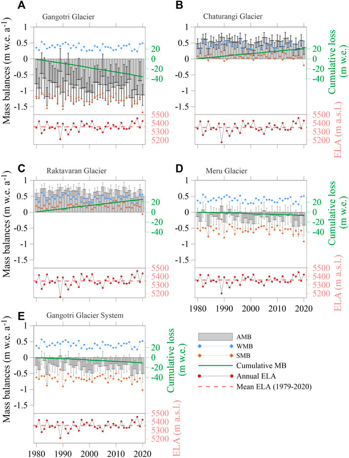
FIGURE 5. Annual and seasonal modelled MBs for (A) Gangotri Glacier, (B) Chaturangi Glacier, (C) Raktavaran Glacier, (D) Meru Glacier and (E) Gangotri Glacier System. Grey bars represent annual MBs along with the associated uncertainties. Blue and red-brown rhombus represent the winter and summer MBs, respectively. Green lines show the cumulative MBs, red dots with black boundaries show the annual ELAs, and the red dashed lines show the mean ELAs over 1979–2020 for the respective glacier.

The mean modelled annual MBs were found as –0.88 ± 0.31, 0.49 ± 0.17, 0.62 ± 0.15, ‒0.17 ± 0.29, and ‒0.27 ± 0.25 m w. e. a^‒ˡ for Gangotri, Chaturangi, Raktavaran, Meru glaciers and Gangotri Glacier System, respectively over 1979–2020. Although the glaciers are in the same catchment (close to each other), but they showed different MBs because of different areal extent, different altitudinal range hence different accumulation and ablation areas. The minimum annual MBs were ‒1.26 ± 0.35, 0.27 ± 0.17, 0.40 ± 0.14, ‒0.44 ± 0.33, and ‒0.57 ± 0.27 m w. e. for the years 2016, 2001, 2001, 2016, and 2016, and the maximum annual MBs were ‒0.44 ± 0.25, 0.68 ±0.12, 0.80 ± 0.13, 0.19 ± 0.22, and 0.06 ± 0.19 m w. e. for the years 1989, 1989, 2005, 1989, and 1989 for Gangotri, Chaturangi, Raktavaran, Meru glaciers and Gangotri Glacier System, respectively (Figure 5). The minimum MBs for Gangotri, Meru and the Gangotri Glacier System were estimated in 2016 due to the higher temperature (3.26°C) and lower precipitation (375.93 mm), and for Chaturangi and Raktavaran glaciers estimated in year 2001 due to the lower precipitation (374.5 mm) and comparatively higher temperature (2.20°C). Similarly, the maximum MBs for Gangotri, Meru and the Gangotri Glacier System estimated in year 1989 due to the lower temperature (1.11°C) and higher precipitation (514.6 mm) and for Chaturangi and Raktavaran glaciers estimated in year 1989 and 2005, respectively due to the lower temperature (1.11, 1.20°C, respectively) and higher precipitation (514.6, 541.6 mm, respectively). The cumulative MBs were ‒35.9 ± 1.96, 20.2 ± 1.12, 25.5 ± 0.94, ‒6.9 ± 1.85, and ‒11.1 ± 1.58 m w. e. for Gangotri, Chaturangi, Raktavaran, Meru glaciers and Gangotri Glacier System, respectively (Figure 5).

Modelled summer MBs (mean) varied from ‒0.84 to ‒1.68 (‒1.25 ± 0.30), ‒0.20 to 0.23 (0.06 ± 0.17), ‒0.06 to 0.37 (0.19 ± 0.14), ‒0.23 to ‒0.92 (‒0.56 ± 0.29), and ‒0.37 to ‒1.02 (‒0.67 ± 0.24) m w. e. a^‒ˡ and the winter MBs (mean) varied from 0.24 to 0.54 (0.38 ± 0.02), 0.27 to 0.61 (0.43 ± 0.02), 0.28 to 0.62 (0.44 ± 0.02), 0.25 to 0.56 (0.39 ± 0.02), and 0.25 to 0.57 (0.40 ± 0.02) m w. e. a^‒ˡ for Gangotri, Chaturangi, Raktavaran, Meru glaciers and Gangotri Glacier System, respectively (Figure 5).

The Gangotri Glacier continuously lost mass for all years over 1979–2020, while the Meru Glacier experienced a few balanced/slightly positive MB years (1982, 1989, 1992, and 2005) (Figures 5A,D). Conversely, the Chaturangi and Raktavaran glaciers showed positive MBs continuously for all years (Figures 5B,C). As a result, the Gangotri Glacier System showed a continuous but moderate mass loss from 1979 to 2020, except for 1989 when the MB was slightly positive (Figure 5E). The exceptional positive MBs on Chaturangi and Raktavaran glaciers, despite a general wastage in the Himalaya, have been discussed in Section 5.1.

4.2 Equilibrium line altitude and accumulation area ratio

The mean modelled ELAs were found to be 5358, 5350, 5347, 5358, and 5356 m a.s.l. for Gangotri, Chaturangi, Raktavaran, Meru glaciers and Gangotri Glacier System, respectively over 1979–2020 (Figure 5). The nearly equal ELAs and their similar interannual variability on all glaciers (Figure 5) were due to the model calibration process where the whole Gangotri Glacier System is calibrated against the geodetic MB (Section 3.3) that resulted in the same distribution of the temperature and precipitation fields on all glaciers. However, the mean annual AARs, which depend on the ratio of ablation and accumulation areas, were quite different, with the values of 45%, 81%, 86%, 54%, and 61% corresponding to an annual mean MBs of ‒0.88, 0.49, 0.62, ‒0.17, and ‒0.27 m w. e. a⁻¹ for Gangotri, Chaturangi, Raktavaran, Meru glaciers, and Gangotri Glacier System, respectively.

Surprisingly, the modelled ELAs on Chaturangi and Raktavaran glaciers are slightly below the debris cover (Figure 7). These glaciers are expected to receive comparatively more solar radiation because of their south-west aspect, resulting in more melting hence higher ELAs than Gangotri and Meru glaciers. As our model provided uniform precipitation and temperature fields hence the accumulation and ablation on all the glaciers, the modelled ELAs on Chaturangi and Raktavaran glaciers are expected to be lower than the actual ELAs or SLAs at the end of ablation season. We delineated the SLAs (see details in Section 3.4) for Chaturangi and Raktavaran glaciers and found that the SLAs are higher than both the debris cover as well as the modelled ELAs. For Chaturangi and Raktavaran glaciers, the mean SLA (delineated for 2013, 2015, 2019 and 2020) and the mean modelled ELA (for same years) differed by 101 m and 112 m, respectively. Modelled ELAs and SLAs on Gangotri Glacier (Section 3.4) as well as some previous studies, comparing modelled ELAs with field-based ELAs, have shown more than 200 m difference among modelled ELAs, delineated SLAs and in situ ELAs (Wang et al., 2017; Azam and Srivastava., 2020). Though, the difference in our modelled ELAs and delineated-SLAs is only around 100 m, yet it is clear that the modelled ELAs (below debris cover) are underestimated; therefore, it is advised to be cautious when this data is used.

The relationships between the modelled MBs, ELAs, and AARs for all glaciers were established individually using 41 years of modelled values (Figure 6). The steady-state ELAs (ELA₀) were also estimated as 5177, 5529, 5838, 5374, and 5267 m a.s.l. for Gangotri, Chaturangi, Raktavaran, Meru glaciers, and the Gangotri Glacier System, respectively using regression fits for zero MB over 1979–2020. The ELA₀ of 5267 m a.s.l. for the Gangotri Glacier System was in good agreement with the ELA₀ of 5280 m a.s.l. for the Dokriani Bamak Glacier (Azam and Srivastava, 2020). Similarly, the steady-state AARs (AAR₀) were 60, 65, 70, 58, and 66% for Gangotri, Chaturangi, Raktavaran, Meru and Gangotri Glacier System, respectively. The AAR₀ values for our study area were well-matched to the AAR₀ ranges (43%–73%) compiled by Pratap et al. (2016) for various Himalayan glaciers.

FIGURE 6

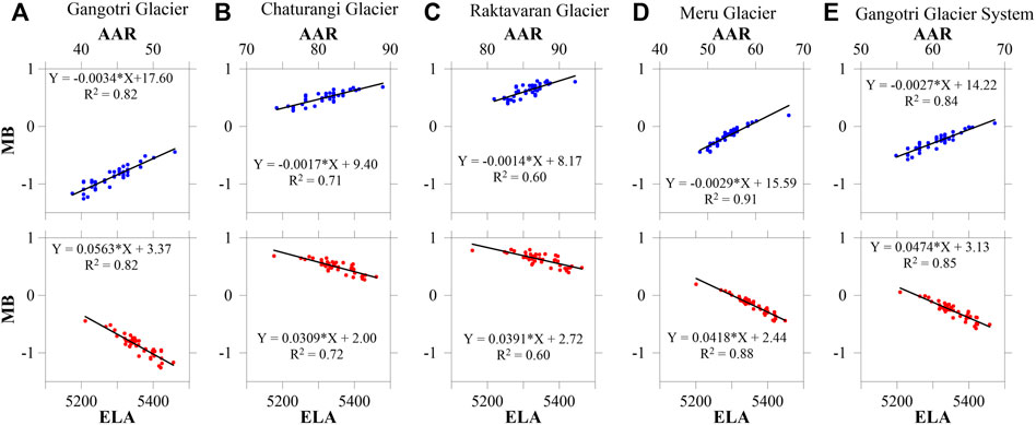
FIGURE 6. ELA (in m a.s.l.) and AAR (in %) relationship with the annual MBs for (A) Gangotri Glacier, (B) Chaturangi Glacier, (C) Raktavaran Glacier, (D) Meru Glacier and (E) Gangotri Glacier System.

5 Discussion

5.1 Positive MBs of fragmented tributary Chaturangi and Raktavaran glaciers

The modelled MBs of Chaturangi and Raktavaran glaciers were positive with mean values of 0.49 ± 0.17 and 0.62 ± 0.15 m w. e. a^‒ˡ, respectively over 1979–2020 (Figure 5). Further, their summer mean MBs were also positive with occasional negative summer MBs (Figure 5). This seems surprising when the Himalayan glaciers have been losing mass over the last 5–6 decades (Azam et al., 2018; Bolch et al., 2019). Chaturangi and Raktavaran are quite big (75 km² and 30 km², respectively) and high-altitude (4,450–6,900 m a.s.l., and 4,600–6,600 m a.s.l, respectively) glaciers. The area-elevation distribution is also very high on both the glaciers hence most of their glacierized area is above ELA (Chaturangi = 81% and Raktavaran = 86% accumulation area, respectively) —giving rise to a very small ablation area exposed to positive summer temperatures (Figures 7B,C). Further, ablation areas are covered by thick debris (∼15% area covering these glaciers from snouts to slightly above ELA) that protects these glaciers from higher melting. This exceptionally high area-elevation distribution coupled with debris-covered tongues resulted in very limited wastage, easily compensated by the large summer accumulation (Figures 7B, 5). Hence, Chaturangi and Raktavaran glaciers showed positive summer mean MBs that further produced positive annual mean MBs. Gangotri and Meru glaciers have significant ablation areas below ELA (45% and 54%, respectively; Figures 7A,D) hence their modelled mean annual MBs were negative. The whole Gangotri Glacier System also has a significant ablation area below ELA (39%, Figure 7E) that produced negative summer MBs resulting in the moderate annual mass loss (Section 4.1).

FIGURE 7

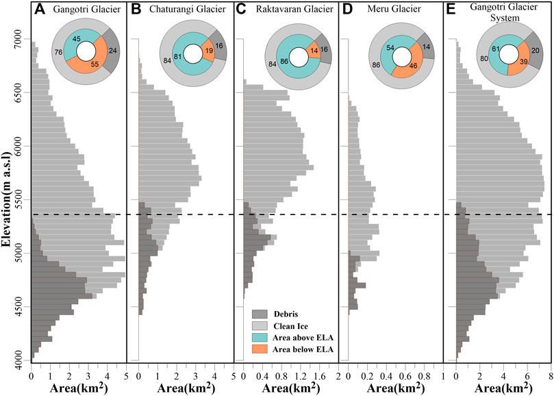
FIGURE 7. The 50-m hypsometry for four selected glaciers (A–D) and the Gangotri Glacier System (E). Light grey bars represent the glacier area, and the dark grey bars represent the debris-covered area on each glacier. The outer pie charts show the percentage of debris-covered and clean-ice glacier surface area, and the inner pie charts show the areas below and above the equilibrium line altitudes (ELAs). The black dashed line is the mean ELA of the Gangotri Glacier System.

The modelled cumulative MBs for the Chaturangi and Raktavaran glaciers were 20.2 ± 1.12 and 25.5 ± 0.94 m w. e, respectively over 1979–2020. These continued cumulative positive MBs must have resulted in terminus advancement through higher ice flux transfer to the terminus, and as a result, both the glaciers must have advanced and re-reconnected to the main Gangotri Glacier trunk, but these are still fragmented from the Gangotri Glacier (Figure 1). Previous literature suggests that Chaturangi, Raktavaran and Meru glaciers were connected to the main Gangotri Glacier in the past and got fragmented from the main glacier (GSI, 2004). Chaturangi Glacier was an independent glacier during the 1960s, then it advanced and attached to the Gangotri Glacier in 1971 (Srivastava, 2012), and then again detached sometime around the early 1990s (Bisht et al., 2020), while Raktavaran seems to be an independent glacier even during the last Little Ice Age (GSI, 2004). The information about the Meru Glacier detachment is not available in the literature. Chaturangi Glacier is having retreat and advance periods however our model—not involving glacier dynamics—cannot provide insights on this. During the field surveys in 2010 (Pottakkal et al., 2014), it was observed that the Chaturangi Glacier snout lies in a steep and deep gorge bounded by unstable steep valley walls. In such a situation, the continuous rockfalls and gushing water probably provide some mechanical ablation to the snout. However, detailed research about Chaturangi Glacier’s snout advance/retreat (Srivastava, 2012) is needed using some sophisticated models including the glacier dynamics and the local topography in the modelling scheme.

We hypothesize that the cumulative positive MBs on Chaturangi and Raktavaran glaciers lead to the glacier advancement and a possible reconnection to the main Gangotri Glacier trunk. Therefore, to determine the impact of the existing unglacierized area between these glaciers and the Gangotri Glacier trunk on modelled MBs, we re-ran the model to reconstruct the MBs assuming that both glaciers are linked with the Gangotri Glacier trunk. This assumption gives an additional ablation area of 0.41 km² on Chaturangi Glacier and 0.59 km² on Raktavaran Glacier. With these additional ablation areas, the modelled mean MBs of 0.47 and 0.55 m w. e. a^‒ˡ were obtained on Chaturangi and Raktavaran glaciers, respectively over 1979–2020. The minor differences of 0.02 m w. e. a^‒ˡ and 0.07 m w. e. a^‒ˡ on Chaturangi and Raktavaran glaciers, respectively show that the advancement has almost no effect on the modelled MBs on these glaciers.

5.2 Assumption of DDF for thick debris having ice cliffs and supra-glacial lakes and suitability of T-index model

Supra-glacial debris surface is ubiquitous on the Himalayan glaciers that strongly impacts glaciers’ response (Scherler et al., 2011; Banerjee and Shankar, 2013). While the thin debris cover of a few millimeters accelerates the melting, the thick debris cover of more than a few centimeters can protect the glacier from higher melting (Shah et al., 2019). It has also been observed that the thick debris-covered glaciers may have ice cliffs and supra-glacial lakes that result in enhanced, localized melting; hence ice cliffs and supra-glacial lakes are considered as the melting hotspots (Buri et al., 2016; Miles et al., 2016). Further, several studies focusing on large-scale glacierized regions have revealed that both debris-covered and clean glaciers experience similar mass wastage (Kääb et al., 2012; Brun et al., 2019), a phenomenon that has been coined as the “debris-cover anomaly” (Pellicciotti et al., 2015; Vincent et al., 2016). This is due to the presence of hotspots on the debris-covered area of some large glaciers that give rise to higher localized melting (Buri et al., 2016; Miles et al., 2016) that compensates for the lower melting on the debris-covered region; therefore, near-similar mass wastage on debris-covered and clean glaciers at regional scale (Kääb et al., 2012).

In Gangotri Glacier System, ice cliffs and supra-glacial lakes are evident only on the lower ablation area (4,000–4,750 m a.s.l.) of the Gangotri Glacier (Figure 1), while the lower ablation area on other glaciers (Meru, Chaturangi and Raktavaran) has debris cover with some occasional hotspots. The estimated area for ice cliffs and supra-glacial lakes on the Gangotri Glacier was 1.09% (with the maximum contribution of 3.9% from the altitude 4,200–4,250 m a.s.l) and 0.5% (with the maximum contribution of 1.6% from the altitude 4,350–4,400 m a.s.l) of total debris cover area (Figure 9), but these have been found to enhance the melting significantly (Buri et al., 2016; Miles et al., 2016; Brun et al., 2018). Therefore, we used DDF_D to compute the MBs of the debris-covered area on all glaciers except the Gangotri Glacier, where we applied DDF_I to compute the MB over the ablation area with prominent ice cliffs and supra-glacial lakes, assuming that the accelerated melt due to hotspots would compensate for the lower melt over the debris-covered area on Gangotri Glacier tongue (Kääb et al., 2012). DDF_I is applied over 4,000–4,750 m a.s.l. because this range has hotspots while the higher range 4,800–5350 m a.s.l. has only debris cover (hence DDF_D was applied).

To check our assumption of DDF_I application for melt generation over the lower debris-covered area on the Gangotri Glacier, we extracted the glacier thinning rates (dh/dt) from Shean et al. (2020) for all four glaciers of our study area as well as for some other glaciers (clean and debris cover) (Figure 8). The thinning patterns on Meru, Chaturangi and Raktavaran glaciers show that the thinning is subdued on these glaciers due to the presence of debris cover over the ablation area (Figure 8B). In agreement, Bhagirathi Kharak and Satopanth glaciers in the same region, which too originate from Chowkhamba Massif (flowing SE, opposite to Gangotri Glacier), also showed subdued thinning over the debris-covered ablation area (Figure 8B). On the other hand, Gangotri Glacier witnessed continued thinning over the lower debris-covered area (Figure 8A). We selected a random clean glacier (inset in Figure 8A) from the same region (60 km NW from Gangotri Glacier System) and a large clean glacier of Durung Drung (68 km²) from the Zanskar Range and compared their thinning patterns with that of Gangotri Glacier. The higher thinning over lower elevations on Gangotri Glacier is analogous to the thinning patterns of a randomly selected clean glacier and Durung Drung Glacier (Figure 8A). This reveals that the lower debris-covered ablation area (4,000–4,750 m a.s.l.) of Gangotri Glacier is wasting its mass like clean glaciers and supports the application of DDF_I for computation of melt over the debris-covered area with prominent melting hotspots. Another geodetic study also suggested that the lower ablation area of Gangotri Glacier showed considerable thickness loss despite thick debris cover on its surface, while other glaciers in the system showed subdued thickness losses over the debris-covered area (Bhattacharya et al., 2016).

FIGURE 8

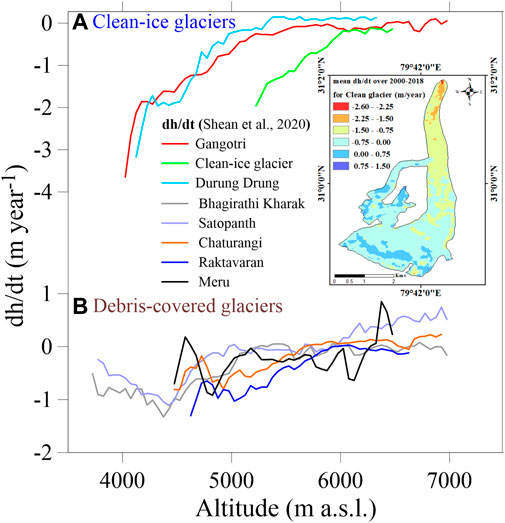
FIGURE 8. (A) Shows the patterns of thinning rate (dh/dt) for clean ice glaciers and (B) shows the patterns of thinning rate for debris-covered glaciers. Inset of panel A is the randomly selected clean glacier.

Though the comparison of thinning patterns (Figure 8A) supports the use of DDF_I for melt computation over the lower debris-covered area on Gangotri Glacier, it is an indirect support and can be questioned. Some studies directly compared the modelled altitudinal MBs with the in situ observations (Azam et al., 2014b; Azam et al., 2019), but such a direct comparison is not possible with geodetic thickness changes as later is the net result of glacier wastage and emergence velocity (Cuffey and Paterson, 2010), that is not accounted in our model. However, our analysis is qualitative, yet it supports the application of T-index model for the MB reconstruction on a large debris-covered glacier with supra-glacial lakes and ice cliffs.

To investigate the impact of our DDF_I application for melt generation over the debris-covered area of Gangotri Glacier, we also ran the model with DDF_D for melt computation over this area. The mean MB with DDF_D was computed as ‒0.60 m w. e. a^‒ˡ against the mean MB of ‒0.88 m w. e. a^‒ˡ with DDF_I for Gangotri Glacier over 1979–2020. The additional ablation contribution, according to our DDF_I assumption, is 32%, which is the combined effect of both ice cliffs and supra-glacial lakes. Our result is in good agreement with the Brun et al. (2018) study, which found a 23% ablation contribution from ice cliffs on Changri Nup Glacier, central Himalaya in Nepal.

5.3 Altitudinal mass balance and gradients

Figure 9 shows the modelled mean altitudinal MB distribution for Gangotri Glacier System over 1979–2020 along with the altitude-wise percentage areal coverage of ice cliffs as well as the supraglacial lakes on the Gangotri Glacier trunk. The altitudinal MB values vary from –8.22 to 1.21 m w. e. for Gangotri, –2.80 to 1.20 m w. e. for Chaturangi, –2.19 to 1.13 m w. e. for Raktavaran, and –3.38 to 1.11 m w. e. for Meru glaciers, and –8.22 to 1.21 m w. e. for Gangotri Glacier System. The highest altitudinal mass loss was observed over the lower ablation area of the main trunk of the Gangotri Glacier (Figure 9). Conversely, the fragmented tributary (Chaturangi, Raktavaran and Meru) glaciers showed relatively less altitudinal mass loss over their lower ablation areas (Figure 9). This is because the lower ablation areas of other glaciers are debris-covered and located at relatively higher altitudes that protect from higher melting on these glaciers (Section 5.1).

FIGURE 9

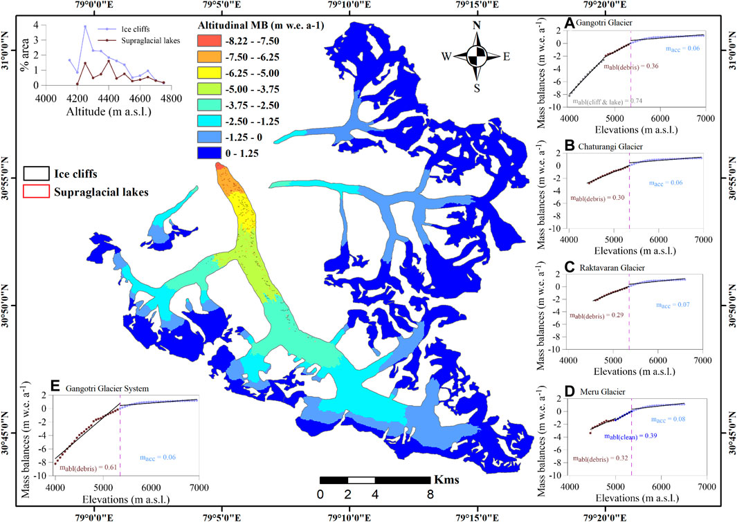
FIGURE 9. Altitudinal MBs and gradient values (in m w. e. per 100 m) in the ablation zone (m_{abl(cliff & lake)}, m_abl(debris) and m_abl(clean) for the thick debris ablation zone having hotspots, debris cover ablation zone and clean ablation zone, respectively) and accumulation zone (m_acc) for (A) Gangotri Glacier, (B) Chaturangi Glacier, (C) Raktavaran Glacier, (D) Meru Glacier and (E) Gangotri Glacier System. Vertical dashed line represents the ELA of each glacier.

We have also estimated MB gradients using the 50-m modelled altitudinal MBs by fitting linear regressions individually for each zone based on the glacier surface morphology (debris or clean ice) and location of ELA (as a demarcation for ablation and accumulation MB gradients) (Figure 9). The MB gradients were estimated as 0.74, 0.36, and 0.06 m w. e. per 100 m for the debris-covered ablation area having hotspots, debris-covered ablation area and accumulation area, respectively for Gangotri Glacier (Figure 9A). Despite considering debris-covered surface with hotspots as clean ice surface (detail in Section 5.2), the Gangotri Glacier MB gradient (0.74 m w. e. per 100 m) was slightly lower than the Dokriani Bamak Glacier MB gradient for the clean ablation [0.91 m w. e. per 100 m, (Azam and Srivastava, 2020)]. The debris cover ablation area of the Chaturangi and Raktavaran glaciers showed very low MB gradients of 0.30 and 0.29 m w. e. per 100 m, respectively because of the substantial debris cover and high altitudes that collectively give rise to less negative altitudinal MBs (Figures 9B,C). For Meru Glacier, MB gradients were calculated for debris-covered ablation area, clean ablation area and accumulation area, and found as 0.32, 0.39, and 0.08 m w. e. per 100 m, respectively (Figure 9D).

For the entire Gangotri Glacier System, the resulted MB gradient for the ablation surface was estimated to be 0.61 m w. e. per 100 m because of its high altitudinal range and high debris cover, which is slightly lower than the MB gradient value for the debris surface of nearby Dokriani Bamak Glacier (0.70 m w. e. per 100 m, Azam and Srivastava, 2020) (Figure 9E). Very low MB gradients in accumulation zones of all glaciers were found because of little or no melting there, and it is attributable solely to snow accumulation for all the glaciers, which is similar on all glaciers due to calibration process (Section 3.3).

5.4 Modelled mass balance sensitivity

The sensitivity of the modelled MB to each parameter was determined by rerunning the model with a uniform change in each model parameter (Oerlemans et al., 1998; Braithwaite and Zhang, 2000; Azam et al., 2014b), while remaining all other model parameters unaltered. These sensitivities were estimated by (Oerlemans et al., 1998):

$\frac{d{B}_a}{d\mu }=\frac{B_a\left({\mu }_H\right)-B_a\left({\mu }_L\right)}{2}(8)$

Where B_a is the average annual and seasonal MB for the period 1979–2020 and µ_H and µ_L are the highest and lowest values of parameters, respectively.

Table 2 provides the computed sensitivities for each model parameter. The sensitivity tests were carried out independently for each glacier. The sensitivity of MB to LR was determined by altering the monthly LR values with the standard deviation of monthly LRs. For the MB sensitivity tests, T_P, T_M and DDFs were modulated by 1°C, 1°C, and 1 mm d⁻¹°C⁻¹, respectively, and P_g was varied by 10%. In this analysis, sensitivity tests were also carried out for input precipitation and temperature, with variations of 10% and 1°C, respectively.

The MBs are most sensitive to T_M with sensitivities of 0.81, 0.25, 0.19, 0.55, and 0.56 m w. e. a^‒ˡ for Gangotri, Chaturangi, Raktavaran, Meru glaciers, and Gangotri Glacier System, respectively (Table 2). The similar sensitivities were also found on the other Himalayan glaciers: MB was most sensitive to T_M with the sensitivities of 0.44 m w. e. a^‒ˡ for the Chhota Shigri Glacier and 0.77 m w. e. a^‒ˡ for the Dokriani Bamak Glacier (Azam et al., 2019; Azam and Srivastava, 2020). Followed by T_M, the modelled MB was most sensitive to the LRs with sensitivities of 0.29, 0.17, 0.14, 0.28, and 0.23 m w. e. a^‒ˡ for Gangotri, Chaturangi, Raktavaran, Meru glaciers, and Gangotri Glacier System, respectively. That is in line with Heynen and others, (2013), which stated that the model is quite sensitive to the LR for the large altitudinal-ranged glaciers. The model was found to be less sensitive to other model parameters (Table 2).

Figures 10A–E shows the relative sensitivity of modelled MB for each model parameter compared to T_M sensitivity, kept as 100%. For the Gangotri Glacier and the whole Gangotri Glacier System, the modelled MBs were least sensitive to DDF_D due to the assumption of a debris surface with hotspots as clean ice (Section 5.2), whereas for the Chaturangi and Raktavaran glaciers, the modelled MBs were least sensitive to DDF_I due to the large coverage of debris cover on the ablation surfaces (Figure 10).

FIGURE 10

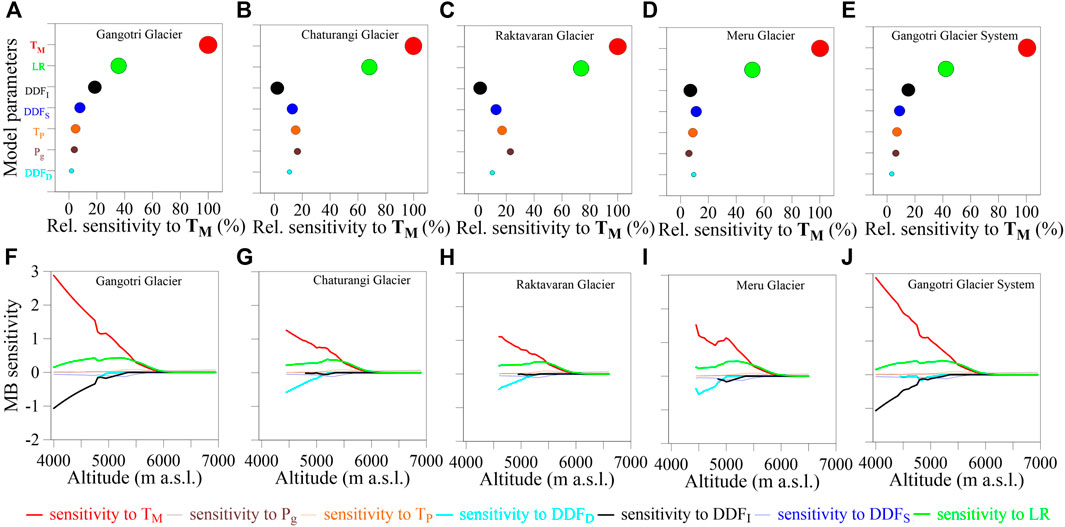
FIGURE 10. Panels (A–E): Bubble plots of relative MB sensitivities for all parameters corresponding to T_M as 100% for Gangotri, Chaturangi, Raktavaran, Meru and Gangotri Glacier System, respectively. Panels (F–J): Altitudinal MB sensitivities for all the parameters for Gangotri, Chaturangi, Raktavaran, Meru and Gangotri Glacier System, respectively.

We also plotted the altitudinal MB sensitivities to all the model parameters (Figures 10F–J). The MB sensitivity to the most sensitive parameter, T_M decreases with altitude, and becomes almost insensitive above 6,200 m a.s.l. for all the glaciers. This is because at lower altitudes the air temperature is usually higher than T_M and there are always some positive temperatures up to 6,200 m a.s.l. Model sensitivity to T_M changes abruptly around 4,800–5000 m a.s.l. on all glaciers because of sudden changes in surface conditions (debris-cover to clean ice or vice versa) (Figure 10I). All glaciers’ sensitivity to LR increases slightly with altitude in the ablation area and decreases with altitude in the accumulation area. The sensitivity to LR varies insignificantly in the debris-covered ablation area (Figures 10G–I) due to the debris cover’s protection (hence less melting and sensitivity); however, at higher altitudes debris-covered area percentage gradually decreases (Figure 7) and thus sensitivity to LR gradually increases (Figures 10F,J). Above this transition zone, where debris-covered and clean-ice areas coexist at the same elevation band, the LR sensitivity gradually decreases with air temperature and becomes zero at around 6,200 m a.s.l.

We assumed the lower debris-covered area with hotspots on Gangotri Glacier to be similar to clean ice (Section 5.2); therefore, the lower debris-covered area on Gangotri Glacier (as well as Gangotri Glacier System) shows high sensitivity to DDF_I instead of DDF_D, that show higher sensitivities on rest of the debris-covered glaciers (Figure 10). The altitudinal MB sensitivity to DDF_S and T_P on all glaciers is negligible. The altitudinal sensitivity analysis clearly indicates that practically all the model parameters become insensitive at higher altitudes (6,200 m a.s.l.), and there is no effect on glacier health.

We also ran the model with 10% and 1°C variation in input precipitation and temperature data, respectively to understand the relative control of precipitation and temperature on the studied glaciers. The MB sensitivities were 0.07, 0.09, 0.09, 0.07, and 0.08 m w. e. a^‒ˡ to a 10% increase in precipitation, while the sensitivities were computed to be ‒0.54, ‒0.23, ‒0.18, ‒0.43, and ‒0.40 m w. e. a^‒ˡ to 1°C increase in temperature for Gangotri, Chaturanga, Raktavaran, Meru glaciers, and Gangotri Glacier System, respectively. We ran the model numerous times to estimate the additional precipitation required to compensate for a 1°C increase in temperature. The results showed that 83%, 32%, 24%, 66%, and 59% increase in precipitation is required to compensate 1°C rise in temperature on the Gangotri, Chaturangi, Raktavaran, Meru glaciers, and Gangotri Glacier System, respectively. The amount of precipitation increase by 59% to compensate for a 1°C temperature rise on the Gangotri Glacier System is in good agreement with the nearby Dokriani Bamak Glacier, where a 49% increase in precipitation was suggested to compensate for a 1°C temperature rise (Azam and Srivastava, 2020). Our results for Chaturangi and Raktavaran glaciers showed good agreement with Braithwaite et al. (2003), who reported a 30–40% increase in precipitation to compensate for the effect of a 1°C temperature rise based on 61 glaciers and ice caps from different regions of the world. The significant precipitation requirements for the Gangotri and Meru glaciers were due to a considerable number of days with temperatures above the T_M, leading to more melting.

5.5 Comparison with other studies

A few studies estimated the MBs of the Gangotri Glacier or Gangotri Glacier System using geodetic and modelling approaches. Our modelled mean MB on the Gangotri Glacier System was ‒0.27 ± 0.25 m w. e. a^‒ˡ over 1979–2020 while Bhattacharya et al. (2016) estimated a mean mass wastage of ‒0.19 ± 0.12 m w. e. a^‒ˡ over 1968–2014 using the geodetic approach. Our model was calibrated using mean MB data from the same study over 2006–2014 (Section 3.3). The slightly higher mass wastage in our study may be attributed to different time periods; nevertheless, the modelled mean MB is in good agreement considering the uncertainty bounds in MBs in both the studies. Another geodetic study estimated a mean mass wastage of ‒0.55 ± 0.42 m w. e. a^‒ˡ on Gangotri Glacier over 1999–2014 (Bhushan et al., 2017). Over the same period, our model showed a higher mean mass wastage of ‒0.89 ± 0.31 m w. e. a^‒ˡ on Gangotri Glacier. However, our modelled MBs on Gangotri Glacier are in better agreement with (Agrawal et al., 2018) who estimated the mean MB of ‒0.98 m w. e. a^‒ˡ on Gangotri Glacier using a simplified energy balance model over 1985–2005 while our study estimated a mean wastage of ‒0.84 ± 0.30 m w. e. a^‒ˡ over the same period. The same study also estimated the mean MB as ‒0.92 m w. e. a^‒ˡ using an ice-flow velocity method over 2001–2014 that is in good agreement with the mean MB of ‒0.87 ± 0.30 m w. e. a^‒ˡ estimated in our study over the same period.

Previous studies estimated a much higher wastage when considering only Gangotri Glacier (Bhushan et al., 2017; Agrawal et al., 2018) compared to Gangotri Glacier System (Bhattacharya et al., 2016) and the same has been observed in our study, but no attention was paid to these significant differences. Our study, focusing on the overall Gangotri Glacier System as well as all individual glaciers explains these large differences. The higher mass wastage on Gangotri Glacier (–0.88 ± 0.31 m w. e. a^‒ˡ) is compensated by the slight mass loss on Meru Glacier (−0.17 ± 0.29 m w.e. a⁻¹) and positive mass budgets on fragmented high-altitude tributary Chaturangi and Raktavaran glaciers (0.49 ± 0.17 and 0.62 ± 0.15 m w. e. a^‒ˡ, respectively) hence the whole Gangotri Glacier System has been experiencing a moderate mass loss of ‒0.27 ± 0.25 m w. e. a^‒ˡ over 1979–2020. This mass wastage is similar to a nearby debris-covered (13% debris surface) Dokriani Bamak Glacier that witnessed a mean mass wastage of ‒0.25 ± 0.37 m w. e. a^‒ˡ over 1979–2018 (Azam and Srivastava, 2020). Further, the modelled mass wastage on Gangotri Glacier System is also in good agreement with the mean geodetic mass wastage of ‒0.37 m w. e. a^‒ˡ in the whole Himalaya over 1975–2010 (Azam et al., 2018).

The Himalayan glaciers have been in general wastage conditions, while the glaciers in the Karakoram Range (west to the Himalaya) are in a near-balanced state at least since 1970s (Azam et al., 2018; Bolch et al., 2019). The near-balanced condition of Karakoram glaciers is linked with the increasing snowfalls (hence more accumulation) due to increased local irrigation (Kumar et al., 2019; Farinotti et al., 2020). With increasing global warming, the Karakoram glaciers also started thinning post-2010, and they are expected to lose their mass in the coming decades (Hugonnet et al., 2021). The positive MBs on Chaturangi and Raktavaran glaciers should not be misunderstood as climate change deniers or compared with Karakoram glaciers. The positive MBs on these fragmented tributary glaciers are due to non-climatic topographic reasons: very high area-altitude distribution and the presence of thick debris cover.

6 Conclusion

The MBs of Gangotri Glacier, its fragmented tributary glaciers (Chaturangi, Raktavaran and Meru glaciers) and the Gangotri Glacier System were reconstructed using T-index model over 1979–2020. Most of the model parameters were taken from the nearby Dokriani Bamak Glacier except T_M and P_g, which were derived by calibrating the modelled MB of the Gangotri Glacier System with the available geodetic MB from Bhattacharya et al. (2016) over 2006–2014. The model was validated using the modelled SLAs against the manually delineated snow line altitudes (SLAs) derived from the Landsat satellite images.

The modelled mean annual MBs were found as –0.88 ± 0.31, 0.49 ± 0.17, 0.62 ± 0.15, ‒0.17 ± 0.29, and ‒0.27 ± 0.25 m w. e. a^‒ˡ for Gangotri, Chaturangi, Raktavaran, Meru glaciers and Gangotri Glacier System, respectively. The mean ELAs were approximately ∼5350 m a.s.l. for all glaciers. The AARs for Gangotri Glacier, Meru Glacier and Gangotri Glacier System were 45%, 54%, and 61%. Conversely, the higher AARs of 81% and 86% on Chaturangi and Raktavaran glaciers, respectively were because of the high-altitude range that resulted in very less area exposed to positive temperature.

The fragmented tributary Chaturangi and Raktavaran glaciers showed positive mean summer and annual MBs due to the high area-elevation distribution and debris-covered tongues. Literature suggests retreat and advance periods on Chaturangi Glacier. Further research, using some sophisticated models including the glacier dynamics and the local topography, is needed to better understand the dynamics of Chaturangi Glacier.

Because of the existence of melting hotspots (ice cliffs and supra-glacial lakes), the debris-covered tongue of the Gangotri Glacier was assumed as a clean-ice surface, and DDF_I was employed to compute the ablation. Our model computed an additional ablation contribution of 32% due to ice cliffs and supra-glacial lakes. The altitudinal MB gradients of our study region were determined to be slightly less than those of other Himalayan glaciers due to the debris-covered ablation surface and high altitudes. The modelled MBs are most sensitive to T_M followed by LR and other parameters (that have quite low sensitivities). The sensitivity analysis showed that the change in annual MBs due to 1°C rise in temperature can be compensated by increasing the precipitation by 83%, 32%, 24%, 66%, and 59% for Gangotri, Chaturangi, Raktavaran, Meru glaciers and Gangotri Glacier System, respectively.

Our study for the first time showed that there are high-altitude, heavily debris-covered fragmented tributary glaciers that might be facing balanced or positive mass budgets in the Himalaya. Further, we also showed that a simple T-index model, with some limitations, can be applied to simulate the MBs of a debris-covered glaciers having ice cliffs and supra-glacial lakes. We stress that the positive MBs on fragmented tributary Chaturangi and Raktavaran glaciers should not be considered as climate change deniers as these MBs are due to topographic settings, and with increasing global warming these glaciers are also expected to waste their ice mass.

Data availability statement

The original contributions presented in the study are included in the article/Supplementary Material, further inquiries can be directed to the corresponding author.

Author contributions

MFA conceived the study. MAH, MFA, and SS developed the model. MAH did the simulations and developed the analysis and figures with the help of MFA and SS. All authors contributed to writing the manuscript.

Acknowledgments

MFA acknowledges the research grants from Space Application Centre (India) and Department of Science and Technology India (CRG/2020/004877). SS is thankful to support from ISRO RESPOND project.

Conflict of insterest

The authors declare that the research was conducted in the absence of any commercial or financial relationships that could be construed as a potential conflict of interest.

Publisher’s note

All claims expressed in this article are solely those of the authors and do not necessarily represent those of their affiliated organizations, or those of the publisher, the editors and the reviewers. Any product that may be evaluated in this article, or claim that may be made by its manufacturer, is not guaranteed or endorsed by the publisher.

References

Agrawal, A., Thayyen, R. J., and Dimri, A. P. (2018). Mass-balance modelling of Gangotri glacier. Geol. Soc. Lond. Spec. Publ. 462 (1), 99–117. doi:10.1144/SP462.1

CrossRef Full Text | Google Scholar

Anslow, F. S., Hostetler, S., Bidlake, W. R., and Clark, P. U. (2008). Distributed energy balance modeling of South Cascade Glacier, Washington and assessment of model uncertainty. J. Geophys. Res. 113 (F2), F02019. doi:10.1029/2007JF000850

CrossRef Full Text | Google Scholar

Azam, M. F., Kargel, J. S., Shea, J. M., Nepal, S., Haritashya, U. K., Srivastava, S., et al. (2021). Glaciohydrology of the himalaya-karakoram. Science 373 (6557), eabf3668. doi:10.1126/science.abf3668

PubMed Abstract | CrossRef Full Text | Google Scholar

Azam, M. F., and Srivastava, S. (2020). Mass balance and runoff modelling of partially debris-covered Dokriani Glacier in monsoon-dominated Himalaya using ERA5 data since 1979. J. Hydrology 590, 125432. doi:10.1016/j.jhydrol.2020.125432

CrossRef Full Text | Google Scholar

Azam, M. F., Wagnon, P., Berthier, E., Vincent, C., Fujita, K., and Kargel, J. S. (2018). Review of the status and mass changes of Himalayan-Karakoram glaciers. J. Glaciol. 64 (243), 61–74. doi:10.1017/jog.2017.86

CrossRef Full Text | Google Scholar

Azam, M. F., Wagnon, P., Vincent, C., Ramanathan, A. L., Favier, V., Mandal, A., et al. (2014b). Processes governing the mass balance of Chhota Shigri Glacier (Western Himalaya, India) assessed by point-scale surface energy balance measurements. Cryosphere 8 (6), 2195–2217. doi:10.5194/tc-8-2195-2014

CrossRef Full Text | Google Scholar

Azam, M. F., Wagnon, P., Vincent, C., Ramanathan, A. L., Kumar, N., Srivastava, S., et al. (2019). Snow and ice melt contributions in a highly glacierized catchment of Chhota Shigri Glacier (India) over the last five decades. J. Hydrology 574, 760–773. doi:10.1016/j.jhydrol.2019.04.075

CrossRef Full Text | Google Scholar

Azam, M. F., Wagnon, P., Vincent, C., Ramanathan, A. L., Linda, A., and Singh, V. B. (2014a). Reconstruction of the annual mass balance of Chhota Shigri Glacier, western Himalaya, India, since 1969. Ann. Glaciol. 55 (66), 69–80. doi:10.3189/2014AoG66A104

CrossRef Full Text | Google Scholar

Banerjee, A., and Shankar, R. (2013). On the response of Himalayan glaciers to climate change. J. Glaciol. 59 (215), 480–490. doi:10.3189/2013JoG12J130

CrossRef Full Text | Google Scholar

Bhaskaran, B., Jones, R. G., Murphy, J. M., and Noguer, M. (1996). Simulations of the Indian summer monsoon using a nested regional climate model: Domain size experiments. Clim. Dyn. 12 (9), 573–587. doi:10.1007/BF00216267

CrossRef Full Text | Google Scholar

Bhattacharya, A., Bolch, T., Mukherjee, K., Pieczonka, T., Kropáček, J., and Buchroithner, M. F. (2016). Overall recession and mass budget of Gangotri Glacier, Garhwal Himalayas, from 1965 to 2015 using remote sensing data. J. Glaciol. 62 (236), 1115–1133. doi:10.1017/jog.2016.96

CrossRef Full Text | Google Scholar

Bhushan, S., Syed, T. H., Kulkarni, A. V., Gantayat, P., and Agarwal, V. (2017). Quantifying changes in the Gangotri Glacier of central Himalaya: Evidence for increasing mass loss and decreasing velocity. IEEE J. Sel. Top. Appl. Earth Obs. Remote Sens. 10 (12), 5295–5306. doi:10.1109/JSTARS.2017.2771215

CrossRef Full Text | Google Scholar

Bisht, H., Kotlia, B. S., Kumar, K., Joshi, L. M., Sah, S. K., and Kukreti, M. (2020). Estimation of the recession rate of Gangotri glacier, Garhwal Himalaya (India) through kinematic GPS survey and satellite data. Environ. Earth Sci. 79 (13), 329. doi:10.1007/s12665-020-09078-0

CrossRef Full Text | Google Scholar

Bolch, T., Shea, J. M., Liu, S., Azam, M. F., Gao, Y., Gruber, S., et al. (2019). in Status and change of the cryosphere in the extended hindu kush Himalaya region” in the hindu kush Himalaya assessment. Editors P. Wester, A. Mishra, A. Mukherji, and A. B. Shrestha (Cham: Springer International Publishing), 209–255. doi:10.1007/978-3-319-92288-1_7

CrossRef Full Text | Google Scholar

Braithwaite, R. J., Zhang, Y., and Raper, S. C. B. (2003). Temperature sensitivity of the mass balance of mountain glaciers and ice caps as a climatological characteristic. Z. für Gletscherkd. Glazialgeol. 38 (1), 35–61.

Google Scholar

Braithwaite, R. J., and Zhang, Y. (2000). Sensitivity of mass balance of five Swiss glaciers to temperature changes assessed by tuning a degree-day model. J. Glaciol. 46 (152), 7–14. doi:10.3189/172756500781833511

CrossRef Full Text | Google Scholar

Brun, F., Berthier, E., Wagnon, P., Kääb, A., and Treichler, D. (2017). A spatially resolved estimate of High Mountain Asia glacier mass balances from 2000 to 2016. Nat. Geosci. 10 (9), 668–673. doi:10.1038/ngeo2999

PubMed Abstract | CrossRef Full Text | Google Scholar

Brun, F., Wagnon, P., Berthier, E., Jomelli, V., Maharjan, S. B., Shrestha, F., et al. (2019). Heterogeneous influence of glacier morphology on the mass balance variability in high mountain Asia. J. Geophys. Res. Earth Surf. 124 (6), 1331–1345. doi:10.1029/2018JF004838

CrossRef Full Text | Google Scholar

Brun, F., Wagnon, P., Berthier, E., Shea, J. M., Berthier, W. W., Kraaijenbrink, P. D. A., et al. (2018). Ice cliff contribution to the tongue-wide ablation of Changri Nup Glacier, Nepal, central Himalaya. Cryosphere 12 (11), 3439–3457. doi:10.5194/tc-12-3439-2018

CrossRef Full Text | Google Scholar

Buri, P., Pellicciotti, F., Steiner, J. F., Miles, E. S., and Immerzeel, W. W. (2016). A grid-based model of backwasting of supraglacial ice cliffs on debris-covered glaciers. Ann. Glaciol. 57 (71), 199–211. doi:10.3189/2016AoG71A059

CrossRef Full Text | Google Scholar

Cuffey, K. M., and Paterson, W. S. B. (2010). The physics of glaciers. Cambridge, Massachusetts: Academic Press.

Google Scholar

Dimri, A. P., Yasunari, T., Kotlia, B. S., Mohanty, U. C., and Sikka, D. R. (2016). Indian winter monsoon: Present and past. Earth-Science Rev. 163, 297–322. doi:10.1016/j.earscirev.2016.10.008

CrossRef Full Text | Google Scholar

Dimri, A. P., Yasunari, T., Wiltshire, A., Kumar, P., Mathison, C., Ridley, J., et al. (2013). Application of regional climate models to the Indian winter monsoon over the Western Himalayas. Sci. Total Environ. 468, S36–S47. doi:10.1016/j.scitotenv.2013.01.040

PubMed Abstract | CrossRef Full Text | Google Scholar

Dobhal, D., Mehta, M., and Srivastava, D. (2013). Influence of debris cover on terminus retreat and mass changes of Chorabari Glacier, Garhwal region, central Himalaya, India. Journal of Glaciology 59 (217), 961–971. doi:10.3189/2013JoG12J180

CrossRef Full Text | Google Scholar

Engelhardt, M., Ramanathan, Al., Eidhammer, T., Kumar, P., Landgren, O., Mandal, A., et al. (2017). Modelling 60 years of glacier mass balance and runoff for Chhota Shigri Glacier, western Himalaya, northern India. J. Glaciol. 63 (240), 618–628. doi:10.1017/jog.2017.29

CrossRef Full Text | Google Scholar

Farinotti, D., Immerzeel, W. W., de Kok, R. J., Quincey, D. J., and Dehecq, A. (2020). Manifestations and mechanisms of the Karakoram glacier anomaly. Nat. Geosci. 13 (1), 8–16. doi:10.1038/s41561-019-0513-5

PubMed Abstract | CrossRef Full Text | Google Scholar

Gaddam, V. K., Kulkarni, A. V., and Gupta, A. K. (2017). Reconstruction of specific mass balance for glaciers in Western Himalaya using seasonal sensitivity characteristic(s). J. Earth Syst. Sci. 126 (4), 55. doi:10.1007/s12040-017-0839-6

CrossRef Full Text | Google Scholar

Gardelle, J., Berthier, E., Arnaud, Y., and Kääb, A. (2013). Region-wide glacier mass balances over the Pamir-Karakoram-Himalaya during 1999–2011. Cryosphere 7 (4), 1263–1286. doi:10.5194/tc-7-1263-2013

CrossRef Full Text | Google Scholar

GSI (Geological Survey of India) (2004) Special publication No. 80, 25. [ISSN 0254-0436, PGSI. 259, 550-2003 (DSK-II)].

Google Scholar

GSI (Geological Survey of India) (2009). Special publication No. 34, 44 [ISSN 0254-0436, PGSI. 308, 500-2009 (DSK-II)].

Google Scholar

Hewitt, K. (2005). The Karakoram anomaly? Glacier expansion and the ‘elevation effect, ’ Karakoram Himalaya. Mt. Res. Dev. 25 (4), 332–340. doi:10.1659/0276-4741(2005)025[0332:TKAGEA]2.0.CO;2

CrossRef Full Text | Google Scholar

Heynen, M., Pellicciotti, F., and Carenzo, M. (2013). Parameter sensitivity of a distributed enhanced temperature-index melt model. Ann. Glaciol. 54 (63), 311–321. doi:10.3189/2013AoG63A537

CrossRef Full Text | Google Scholar

Hock, R., and Holmgren, B. (2005). A distributed surface energy-balance model for complex topography and its application to Storglaciären, Sweden. J. Glaciol. 51 (172), 25–36. doi:10.3189/172756505781829566

CrossRef Full Text | Google Scholar

Hock, R. (2003). Temperature index melt modelling in mountain areas. J. Hydrology 282 (1–4), 104–115. doi:10.1016/S0022-1694(03)00257-9

CrossRef Full Text | Google Scholar

Hugonnet, R., McNabb, R., Berthier, E., Menounos, B., Nuth, C., Girod, L., et al. (2021). Accelerated global glacier mass loss in the early twenty-first century. Nature 592 (7856), 726–731. doi:10.1038/s41586-021-03436-z

PubMed Abstract | CrossRef Full Text | Google Scholar

Immerzeel, W. W., Wanders, N., Lutz, A. F., Shea, J. M., and Bierkens, M. F. P. (2015). Reconciling high-altitude precipitation in the upper Indus basin with glacier mass balances and runoff. Hydrol. Earth Syst. Sci. 19 (11), 4673–4687. doi:10.5194/hess-19-4673-2015

CrossRef Full Text | Google Scholar

Jennings, K. S., Winchell, T. S., Livneh, B., and Molotch, N. P. (2018). Spatial variation of the rain–snow temperature threshold across the Northern Hemisphere. Nat. Commun. 9 (1), 1148. doi:10.1038/s41467-018-03629-7

PubMed Abstract | CrossRef Full Text | Google Scholar

Kääb, A., Berthier, E., Nuth, C., Gardelle, J., and Arnaud, Y. (2012). Contrasting patterns of early twenty-first-century glacier mass change in the Himalayas. Nature 488 (7412), 495–498. doi:10.1038/nature11324

PubMed Abstract | CrossRef Full Text | Google Scholar

King, O., Bhattacharya, A., Bhambri, R., and Bolch, T. (2019). Glacial lakes exacerbate Himalayan glacier mass loss. Sci. Rep. 9 (1), 18145. doi:10.1038/s41598-019-53733-x

PubMed Abstract | CrossRef Full Text | Google Scholar

Kotlia, B. S., Singh, A. K., Joshi, L. M., and Bisht, K. (2018). Precipitation variability over Northwest Himalaya from ∼4.0 to 1.9 ka BP with likely impact on civilization in the foreland areas. J. Asian Earth Sci. 162, 148–159. doi:10.1016/j.jseaes.2017.11.025

CrossRef Full Text | Google Scholar

Kuhn, M. (1987). Micro-meteorological conditions for snow melt. J. Glaciol. 33 (113), 24–26. doi:10.3189/S002214300000530X

CrossRef Full Text | Google Scholar

Kumar, A., Negi, H. S., and Kumar, K. (2021). Long-term (∼40 years) mass balance appraisal and response of the Patsio glacier, in the Great Himalayan region towards climate change. J. Earth Syst. Sci. 130 (1), 50. doi:10.1007/s12040-021-01555-9

CrossRef Full Text | Google Scholar

Kumar, P., Saharwardi, M. S., Banerjee, A., Azam, M. F., Dubey, A. K., and Murtugudde, R. (2019). Snowfall variability dictates glacier mass balance variability in himalaya-karakoram. Sci. Rep. 9 (1), 18192. doi:10.1038/s41598-019-54553-9

PubMed Abstract | CrossRef Full Text | Google Scholar

Litt, M., Shea, J., Wagnon, P., Steiner, J., Koch, I., Stigter, E., et al. (2019). Glacier ablation and temperature indexed melt models in the Nepalese Himalaya. Sci. Rep. 9 (1), 5264. doi:10.1038/s41598-019-41657-5

PubMed Abstract | CrossRef Full Text | Google Scholar

Mandal, A., Angchuk, T., Azam, M. F., Ramanathan, Al., Wagnon, P., Soheb, M., et al. (2022). 11-year record of wintertime snow surface energy balance and sublimation at 4863 m a.s.l. on Chhota Shigri Glacier moraine (Western Himalaya, India). Snow/Energy Balance Obs/Modelling 16, 3775. doi:10.5194/tc-2021-386

CrossRef Full Text | Google Scholar

Mandal, A., Ramanathan, Al., Azam, M. F., Angchuk, T., Soheb, M., Kumar, N., et al. (2020). Understanding the interrelationships among mass balance, meteorology, discharge and surface velocity on Chhota Shigri Glacier over 2002–2019 using in situ measurements. J. Glaciol. 66 (259), 727–741. doi:10.1017/jog.2020.42

CrossRef Full Text | Google Scholar

Maurer, J. M., Schaefer, J. M., Rupper, S., and Corley, A. (2019). Acceleration of ice loss across the Himalayas over the past 40 years. Sci. Adv. 5 (6), eaav7266. doi:10.1126/sciadv.aav7266

PubMed Abstract | CrossRef Full Text | Google Scholar

Miles, E. S., Pellicciotti, F., Willis, I. C., Steiner, J. F., Buri, P., and Arnold, N. S. (2016). Refined energy-balance modelling of a supraglacial pond, Langtang Khola, Nepal. Ann. Glaciol. 57 (71), 29–40. doi:10.3189/2016AoG71A421

CrossRef Full Text | Google Scholar

Negi, H. S., Thakur, N. K., Ganju, A., and Snehmani, (2012). Monitoring of Gangotri glacier using remote sensing and ground observations. J. Earth Syst. Sci. 121 (4), 855–866. doi:10.1007/s12040-012-0199-1

CrossRef Full Text | Google Scholar

Nuimura, T., Sakai, A., Taniguchi, K., Nagai, H., Lamsal, D., Tsutaki, S., et al. (2015). The GAMDAM Glacier Inventory: A quality-controlled inventory of asian glaciers. Cryosphere 9 (3), 849–864. doi:10.5194/tc-9-849-2015

CrossRef Full Text | Google Scholar

Oerlemans, J., Anderson, B., Hubbard, A., Huybrechts, P., Jóhannesson, T., Knap, W. H., et al. (1998). Modelling the response of glaciers to climate warming. Clim. Dyn. 14 (4), 267–274. doi:10.1007/s003820050222

CrossRef Full Text | Google Scholar

Oerlemans, J. (2001). Glaciers and climate change. Boca Raton, Florida: CRC Press.

Google Scholar

Ohmura, A. (2001). Physical basis for the temperature-based melt-index method. J. Appl. Meteor. 40 (4), 753–761. doi:10.1175/1520-0450(2001)040<0753:pbfttb>2.0.co;2

CrossRef Full Text | Google Scholar

Oulkar, S. N., Thamban, M., Sharma, P., Pratap, B., Singh, A. T., Patel, L. K., et al. (2022). Energy fluxes, mass balance, and climate sensitivity of the Sutri Dhaka Glacier in the Western Himalaya. Front. Earth Sci. (Lausanne). 10, 949735. doi:10.3389/feart.2022.949735

CrossRef Full Text | Google Scholar

Pellicciotti, F., Brock, B., Strasser, U., Burlando, P., Funk, M., and Corripio, J. (2005). An enhanced temperature-index glacier melt model including the shortwave radiation balance: Development and testing for haut glacier d’arolla, Switzerland. J. Glaciol. 51 (175), 573–587. doi:10.3189/172756505781829124

CrossRef Full Text | Google Scholar

Pellicciotti, F., Stephan, C., Miles, E., Herreid, S., Immerzeel, W. W., and Bolch, T. (2015). Mass-balance changes of the debris-covered glaciers in the Langtang Himal, Nepal, from 1974 to 1999. J. Glaciol. 61 (226), 373–386. doi:10.3189/2015JoG13J237

CrossRef Full Text | Google Scholar

Pottakkal, J. G., Ramanathan, A., Singh, V. B., Sharma, P., Azam, M. F., and Linda, A. (2014). Characterization of subglacial pathways draining two tributary meltwater streams through the lower ablation zone of Gangotri glacier system, Garhwal Himalaya, India. Curr. Sci. 2014, 613–621.

Google Scholar

Pratap, B., Dobhal, D. P., Bhambri, R., Mehta, M., and Tewari, V. C. (2016). Four decades of glacier mass balance observations in the Indian Himalaya. Reg. Environ. Change 16 (3), 643–658. doi:10.1007/s10113-015-0791-4

CrossRef Full Text | Google Scholar

Pratap, B., Dobhal, D. P., Mehta, M., and Bhambri, R. (2015). Influence of debris cover and altitude on glacier surface melting: A case study on Dokriani glacier, central Himalaya, India. Ann. Glaciol. 56 (70), 9–16. doi:10.3189/2015AoG70A971

CrossRef Full Text | Google Scholar

Pratap, B., Sharma, P., Patel, L., Singh, A. T., Gaddam, V. K., Oulkar, S., et al. (2019). Reconciling high glacier surface melting in summer with air temperature in the semi-arid zone of western Himalaya. Water 11 (8), 1561. doi:10.3390/w11081561

CrossRef Full Text | Google Scholar

Racoviteanu, A. E., Rittger, K., and Armstrong, R. (2019). An automated approach for estimating snowline altitudes in the Karakoram and eastern Himalaya from remote sensing. Front. Earth Sci. (Lausanne). 7, 220. doi:10.3389/feart.2019.00220

CrossRef Full Text | Google Scholar

Ragettli, S., Pellicciotti, F., Bordoy, R., and Immerzeel, W. W. (2013). Sources of uncertainty in modeling the glaciohydrological response of a Karakoram watershed to climate change: Sources of uncertainty in glaciohydrological modeling. Water Resour. Res. 49 (9), 6048–6066. doi:10.1002/wrcr.20450

CrossRef Full Text | Google Scholar

Sakai, A., and Fujita, K. (2017). Contrasting glacier responses to recent climate change in high-mountain Asia. Sci. Rep. 7 (1), 13717–13718. doi:10.1038/s41598-017-14256-5

PubMed Abstract | CrossRef Full Text | Google Scholar

Scherler, D., Bookhagen, B., and Strecker, M. R. (2011). Spatially variable response of Himalayan glaciers to climate change affected by debris cover. Nat. Geosci. 4 (3), 156–159. doi:10.1038/ngeo1068

CrossRef Full Text | Google Scholar

Shah, S. S., Banerjee, A., Nainwal, H. C., and Shankar, R. (2019). Estimation of the total sub-debris ablation from point-scale ablation data on a debris-covered glacier. J. Glaciol. 65 (253), 759–769. doi:10.1017/jog.2019.48

CrossRef Full Text | Google Scholar

Shea, J. M., Immerzeel, W. W., Wagnon, P., Vincent, C., and Bajracharya, S. (2015). Modelling glacier change in the Everest region, Nepal Himalaya. Cryosphere 9 (3), 1105–1128. doi:10.5194/tc-9-1105-2015

CrossRef Full Text | Google Scholar

Shean, D. E., Bhushan, S., Montesano, P., Rounce, D. R., Arendt, A., and Osmanoglu, B. (2020). A systematic, regional assessment of high mountain Asia glacier mass balance. Front. Earth Sci. (Lausanne). 7, 363. doi:10.3389/feart.2019.00363

CrossRef Full Text | Google Scholar

Shugar, D. H., Burr, A., Haritashya, U. K., Kargel, J., Watson, C. S., Kennedy, M. C., et al. (2020). Rapid worldwide growth of glacial lakes since 1990. Nat. Clim. Chang. 10 (10), 939–945. doi:10.1038/s41558-020-0855-4

CrossRef Full Text | Google Scholar

Singh, M. K., Gupta, R. D., and Ganju, A. (2013). Extraction of high-resolution DEM from Cartosat-1 stereo imagery using rational math model and its accuracy assessment for a part of snow-covered NW-Himalaya. J Remote Sens GIS (JORSG) 4 (2), 22–34.

Google Scholar

Singh, P., Haritashya, U. K., Kumar, N., and Singh, Y. (2006). Hydrological characteristics of the Gangotri Glacier, central himalayas, India. J. Hydrology 327 (1–2), 55–67. doi:10.1016/j.jhydrol.2005.11.060

CrossRef Full Text | Google Scholar

Singh, P., Kumar, N., and Arora, M. (2000). Degree–day factors for snow and ice for Dokriani glacier, garhwal himalayas. J. Hydrology 235(1-2), pp.1–11. doi:10.1016/S0022-1694(00)00249-3

CrossRef Full Text | Google Scholar

Srivastava, D. (2012). Status report on Gangotri Glacier science and engineering research board, 3. New Delhi: Department of Science and TechnologyHimalayan Glaciology Technical Report, 21–25.

Google Scholar

Srivastava, S., and Azam, M. F. (2022a). Functioning of glacierized catchments in monsoon and alpine regimes of Himalaya. J. Hydrology 609, 127671. doi:10.1016/j.jhydrol.2022.127671

CrossRef Full Text | Google Scholar

Srivastava, S., and Azam, M. F. (2022b). Mass- and energy-balance modeling and sublimation losses on Dokriani Bamak and Chhota Shigri glaciers in Himalaya since 1979. Front. Water 4, 874240. doi:10.3389/frwa.2022.874240

CrossRef Full Text | Google Scholar

Srivastava, S., Garg, P. K., and Azam, M. F. (2022). Seven decades of dimensional and mass balance changes on Dokriani Bamak and Chhota Shigri glaciers, Indian Himalaya, using satellite data and modelling. J. Indian Soc. Remote Sens. 50, 37–54. doi:10.1007/s12524-021-01455-x

CrossRef Full Text | Google Scholar

Stumm, D., Joshi, S. P., Gurung, T. R., and Silwal, G. (2021). Mass balances of yala and rikha samba glaciers, Nepal, from 2000 to 2017. Earth Syst. Sci. Data 13 (8), 3791–3818. doi:10.5194/essd-13-3791-2021

CrossRef Full Text | Google Scholar

Tawde, S. A., Kulkarni, A. V., and Bala, G. (2016). Estimation of glacier mass balance on a Basin scale: An approach based on satellite-derived snowlines and a temperature index model. Curr. Sci. 111 (12), 1977–1989. doi:10.18520/cs/v111/i12/1977-1989

CrossRef Full Text | Google Scholar

Van den Broeke, M., Bus, C., Ettema, J., and Smeets, P. (2010). Temperature thresholds for degree-day modelling of Greenland ice sheet melt rates: Greenland melt factors. Geophys. Res. Lett. 37 (18). doi:10.1029/2010GL044123

CrossRef Full Text | Google Scholar

Vincent, C., Soruco, A., Azam, M. F., Basantes-Serrano, R., Jackson, M., Kjøllmoen, B., et al. (2018). A nonlinear statistical model for extracting a climatic signal from glacier mass balance measurements. J. Geophys. Res. Earth Surf. 123 (9), 2228–2242. doi:10.1029/2018JF004702

CrossRef Full Text | Google Scholar

Vincent, C., Wagnon, P., Shea, J. M., Immerzeel, W. W., Kraaijenbrink, P., Shrestha, D., et al. (2016). Reduced melt on debris-covered glaciers: Investigations from Changri Nup Glacier, Nepal. Cryosphere 10 (4), 1845–1858. doi:10.5194/tc-10-1845-2016

CrossRef Full Text | Google Scholar

Wagnon, P., Brun, F., Khadka, A., Berthier, E., Shrestha, D., Vincent, C., et al. (2021). Reanalysing the 2007–19 glaciological mass-balance series of Mera Glacier, Nepal, Central Himalaya, using geodetic mass balance. J. Glaciol. 67 (261), 117–125. doi:10.1017/jog.2020.88

CrossRef Full Text | Google Scholar

Wang, S., Yao, T., Tain, L., and Pu, J. (2017). Glacier mass variation and its effect on surface runoff in the Beida River catchment during 1957–2013. J. Glaciol. 63 (239), 523–534. doi:10.1017/jog.2017.13

CrossRef Full Text | Google Scholar

Zemp, M., Frey, H., Gärtner-Roer, I., Nussbaumer, S. U., Hoelzle, M., Paul, F., et al. (2015). Historically unprecedented global glacier decline in the early 21st century. J. Glaciol. 61 (228), 745–762. doi:10.3189/2015jog15j017

CrossRef Full Text | Google Scholar

Zhao, H., Yang, W., Yao, T., Tian, L., and Xu, B. (2016). Dramatic mass loss in extreme high-elevation areas of a Western Himalayan glacier: Observations and modeling. Sci. Rep. 6, 30706. doi:10.1038/srep30706

PubMed Abstract | CrossRef Full Text | Google Scholar