Railway traffic monitoring with trackside fiber-optic cable by distributed acoustic sensing Technology

Introduction

The growing freight volume conveyed by railway systems and the increase of high-speed trains demand more reliable train dynamics monitoring. Currently, railway traffic monitoring in use require the integration of both onboard and wayside measurement as well as data transfer in between them (Ulianov et al., 2018). Conventionally, in the aspect of large-scale railway position monitoring, onboard satellite-based positioning systems such as Global Positioning Satellite (GPS) play a fundamental role. However, when trains go through tunnels or mountains, GPS positioning could be less accurate, or even unreceivable (Sasani et al., 2015). For more stable and real-time monitoring purposes, on a small-scale aspect, magnetic beacons are deployed on railway sleepers as counters to determine if a train has passed (Bruni et al., 2007). Nonetheless, magnetic beacons may suffer from Electromagnetic Interference and lead to missed or wrong messages (Yüksel et al., 2018). Onboard speedometers or accelerometers can measure precise velocity information and need wireless transmission conditions, which could be disrupted due to wireless interference (Baldini et al., 2010).

Recently, Distributed Acoustic Sensing (DAS) technology has been extensively used in the seismological community (Dou et al., 2017; Zeng et al., 2017; Martin et al., 2018; Ajo-Franklin et al., 2019; Zhan, 2019; Lindsey et al., 2017; Spica et al., 2020). When a DAS interrogator is connected to a fiber-optic cable, laser pulses are sent. Subsequently, Rayleigh back-scattered phase shifts are measured and converted to axle strain or strain rate, thereby, the sensing cable becomes a dense array with meter-scale spatial resolutions (Parker et al., 2014). With the use of the dense array features, DAS records high-fidelity seismic wavefields and can be applied in event monitoring, such as aftershock detection (Li et al., 2021; Lv et al., 2022), icequake detection (Walter et al., 2020; Hudson et al., 2021), and urban traffic monitoring (Lindsey et al., 2020). Another advantage of DAS is in its convenient mode of deployment, whereby, widespread existing telecommunication cables can be utilized as dense array sensors, especially in highly-built cities (Lindsey et al., 2020; Song et al., 2021). It is worth noting that urban-scale DAS applications are not limited to vehicle traffic monitoring (Chambers, 2020; van den Ende et al., 2021) and interferometry studies (Dou et al., 2017; Song et al., 2021), but other moving sources like subways (Ferguson et al., 2020) and railway trains (Cedilnik et al., 2018; Wiesmeyr et al., 2020). The trackside cables connected to an interrogator can provide researchers with the opportunity to record train-induced signals, and monitor the location and speed of trains, towards enhancing the train control system.

In previous seismological studies on train-induced signals, the characteristics of the signal itself have attracted extensive attention (Fuchs and Bokelmann, 2017; Lavoué et al., 2020; Jiang et al., 2022). Another idea is to utilize train-induced signals as strong noise source in ambient noise tomography (Quiros et al., 2016; Brenguier et al., 2019; Liu et al., 2021; Sager et al., 2022). Compared to the aforementioned, railway traffic monitoring (i.e., train detection and speed estimation) using DAS could help select proper noise windows for seismic interferometry applications using noise generated from moving trains as source. Trackside DAS recordings require a lot of man-hour inspection/observation to extract the locations of moving trains; this necessitates the need to develop automatic methods for monitoring railway traffic using the high-volume original waveform data. Given that the train-induced signals are spatially continuous, and leave data “footprints” as linear features in the DAS recordings, the Kalman filter has been suggested to be an effective approach to extracting the tracks of individual trains (Wiesmeyr et al., 2020), yet the method may not achieve stable track predictions when it comes to significant speed variant cases. In addition, the method may not accurately extract/predict the locations from cross superimposed signals (Iswanto and Li, 2017), which could be the case when two trains from opposite directions move and pass each other. Train-induced signals in the “waterfall diagram” can be cut out and the signal front over time can be aligned, thereby the speed change could be extracted using spectral shifts (Cedilnik et al., 2018), yet the method requires accurate alignment of the train-induced signal fronts and the calculation of speeds are not in an automatic manner. Similar issues also apply to vehicle monitoring studies where array beamforming technique has been tested and proven to be effective in investigating traffic patterns, and dealing with heavy traffic scenarios (Chambers, 2020; Ende, 2021; van den Ende and Ampuero, 2021).

In this study, we use time-domain beamforming procedure to estimate the short-term average over long-term average traces (STA/LTA; Allen, 1978) of DAS waveform data, to extract the location and speed of individual trains, and demonstrate the effectiveness and stability of our method. In addition, our method can extract the footprint of speed variant trains by constantly moving the subarrays with acceptable real-time performance. Therefore, we first introduce the observation system and further show several typical signals induced by different kinds of trains. Thereafter, the detection and speed estimation are done by the beamforming method. In a bid to demonstrate the reliability of our method, we compare the detection results with the train schedules. Finally, we test the impacts of different signal-to-noise ratio levels and array apertures on beamforming performance, and discuss the applicability of our method.

Data

The experimental site for our study is located ∼5 km north of Hangzhou Railway Station, Hangzhou, Eastern China. Towards the North, the rail tracks run directly underneath NE-SW trending Desheng expressway, while in the south lies the maintenance Depot for Electric Multiple Unit (EMU) trains (Figure 1). We connect the interrogator (HiFi-DAS provided by Puniutech) with an existing trackside telecommunication cable set at a 2-m channel spacing, and calibrate the cable into 1001 sensors. The cable is protected by polyvinyl chloride conduits underground. The data is acquired at a sampling rate of 50 Hz and the gauge length is 10 m. Strain data are continuously recorded over a period of 6 days in 2 different stages, starting from 23rd to 26th in August 2021 and 2nd to 3rd in September 2021, respectively.

FIGURE 1

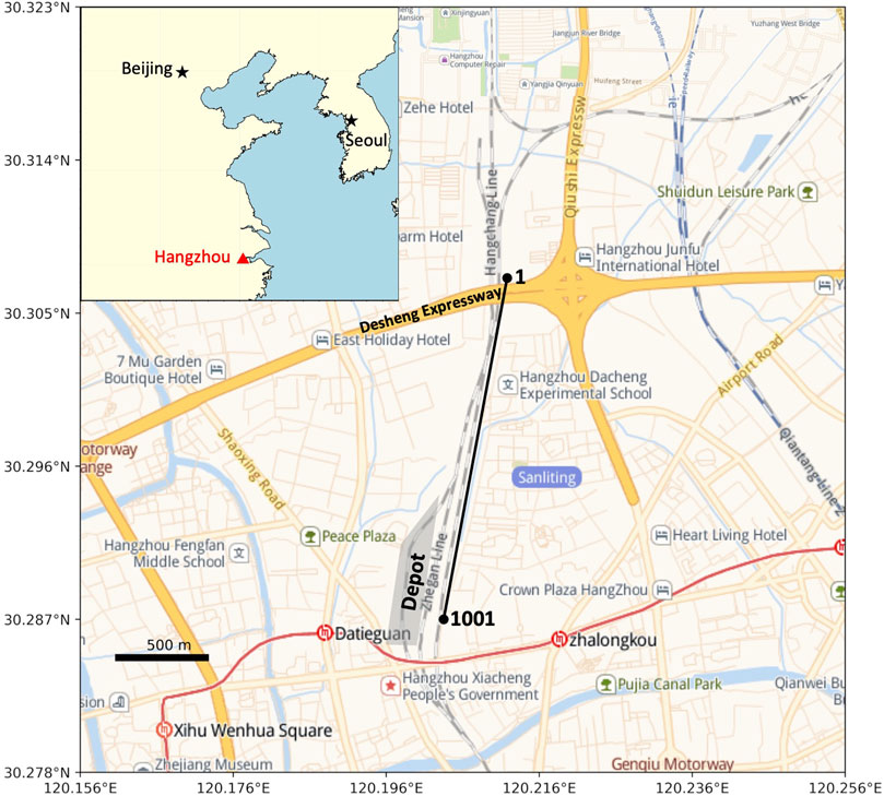
FIGURE 1. Map showing the location of the fiber-optic cable (black line) 5 km north of Hangzhou station (https://lbs.amap.com/demo/javascript-api/example/map/map-english/). Grey shade denotes the Depot. The numbers in black are the start and end channel numbers. The alternating grey and white lines are railway roads (Hanghang Line, Zhegan Line). The blue arrow indicates the direction of the train station. The yellow solid lines denote expressways, and Desheng Expressway is marked where the cable segment from channel 1 to channel 200 lies. Hangzhou (red triangle) and other major cities (black star) are also marked on the inset map.

A 1-h DAS record for a heavy-traffic period is shown in Figure 2. We could easily identify the train-induced, quasi-static deformation signals, leaving the “footprint” of passing trains across the array. The slope of the track can be considered as the speed of individual trains, and in total, there are 13 identical slant lines which demonstrate that the trains pass our array at near constant speeds. From ∼ Ch1-130, there are persistent noises that could have been generated by high-frequency vehicle traffic on Desheng expressway, yet the train-induced signals are still visible. At 11:30, there is an indication that a train moves at low-speed comes from north to south at ∼5 km/h, and fades away at ∼ Ch400. This is conceived to be an EMU parking event for maintenance to the Depot in the south.

FIGURE 2

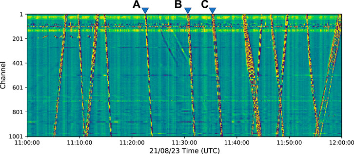
FIGURE 2. One-hour DAS data records under a heavy railway traffic scenario. The reverse blue triangles mark three typical train events shown in Figure 3 (corresponding to (A–C) from left to right).

Trains passing through the site include 8 or 16-wagon EMUs which is powered by each unit (∼26 m in length), and the conventional or locomotive-hauled trains which typically consist of −18—21 wagons powered by the locomotive, individually. Figures 3A–C show raw waveforms recorded at Ch500 due to wagon 8, wagon 16 (from the EMU), and a conventional train, respectively. We then compute their spectrograms (Figures 3D–F) and observe that the signals cover the entire frequency band. In all the 3 cases earlier mentioned (Figure 3), no main frequency is identical and the equal-distance spectral lines observed using seismometers (in the work of Fuchs and Bokelmann, 2017) are also clear in our DAS observations. The distance in-between the spectral lines was suggested to be related to the train speed and the length of bogies (Lavoué et al., 2020). Previous studies have shown that the peaks of train-induced signals correspond to the number of bogies, usually the number of wagons plus 1 (Kowarik et al., 2020; Lavoué et al., 2020). To reduce the influence of high-frequency noise, we apply a 5 Hz lowpass filter on the three waveform signals, thereby enhancing the relatively long-period train-induced signals. After filtering, we could observe clearer periodic signals and peaks (Figures 3G–I), where the peaks correspond to the 9th (8-wangon EMU), 17th (16-wagon EMU), and 21st (20-wagon conventional train) bogies.

FIGURE 3

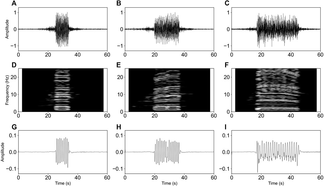
FIGURE 3. Typical train-induced signals of CH500 (A–C), their spectrograms (D–F), and lowpass filtered signals (G–I). The blue circles denote peaks.

Materials and method

Though we could manually identify trains “footprints” from raw waveform DAS data, however, it is still a challenge to detect train-induced events and estimate their speeds automatically. In our experiment, trackside cables are linearly distributed, and as an ultra-dense array, so it is suitable to use the beamforming approach to transfer the raw data to the time-velocity domain whose results are known as vespagram (eg., Rost and Thomas, 2002). The method shifts the phase of each waveform with respect to a range of velocities and then stack the time-shifted waveforms as a beam, whereby the vespagram is the result of all beams calculated all over the speed range (Meng and Ben-Zion, 2018; Nayak and Ajo-Franklin, 2021; van den Ende and Ampuero, 2021). Among the beams, the maximum value of the beampower corresponds to the apparent velocity and event detection time. The beamforming approach has been applied in the vehicle traffic monitoring fields (Chambers, 2020; van den Ende and Ampuero, 2021).

The waveforms are relatively not coherent in the DAS recordings (Figure 4A). Researchers would like to do some pre-processing on the raw data, such as median filter (Chambers, 2021; Nayak and Ajo-Franklin, 2021), or some kind of normalization and smoothing like what Chambers (2020) did by measuring the signal envelopes. Instead of that, we use STA/LTA traces to squeeze signal phases and enhance/equalize the amplitude. The time-domain beamforming technique stacks all the channel data, because the amplitude of the train-induced signals is so high that even the recordings with large noise levels still can help. We didn’t find the data suffer from non-linear behaviors or spiking. Furthermore, we have tested a 7-channel time-domain median filter on our data (Nayak and Ajo-Franklin, 2021), and we didn’t find differences on the results. Compared to signals generated by vehicle, train-induced signals are relatively more complex, which is mainly due to longer periods (vehicle signals with 1 period, trains at least more than 8 periods) and duration of the signal (vehicle less than 1 s, trains longer than 10 s in our study). We use the whole array data to beamform the signals generated from the EMU, having a speed ranging from 10 to 150 km/h, with speed interval of 1 km/h. Typical vespagrams generated from a set of raw and processed signals are shown in Figures 4C,D. A long duration of the train-induced signals could lead to low resolution on the vespagram. While after exploiting the STA/LTA algorithm on the raw data, the resolution on the vespagram is improved. To increase the sensitivity of arrivals, the STA is set as 0.1 s, while the LTA is set as 50 s, longer than the duration of the slowest train. After the processing, the signals are better enhanced and centered at arrivals, while the phases are squeezed. Next, we beamform the STA/LTA traces and the vespagram results show a better temporal resolution. The detection time is around the estimated maximum beampower at the centre of the array. We further extract the maximum value along the time axis and build the time-beampower curve (Figures 4E,F). We could observe that the curve becomes smoother and the peak becomes more prominent after the STA/LTA calculation. We select two threshold parameters namely, prominence and distance, to constrain the find-peak algorithm to estimate the maximum beampower (Virtanen et al., 2020). The prominence is used to constrain the maximum difference between the peaks and saddles, and the distance is the time difference to constrain the corresponding time of the peaks and saddles within the time distance (van den Ende and Ampuero, 2021; Virtanen et al., 2020). When we select a small time-distance parameter, three detection results appear in the time-beampower curve of computed from the raw data (Figure 4E). Meanwhile, after calculating the STA/LTA, the signals are squeezed as sharp impulses like generated by point sources, we then obtain a more stable detection performance result from the time-beampower curve (Figure 4F).

FIGURE 4

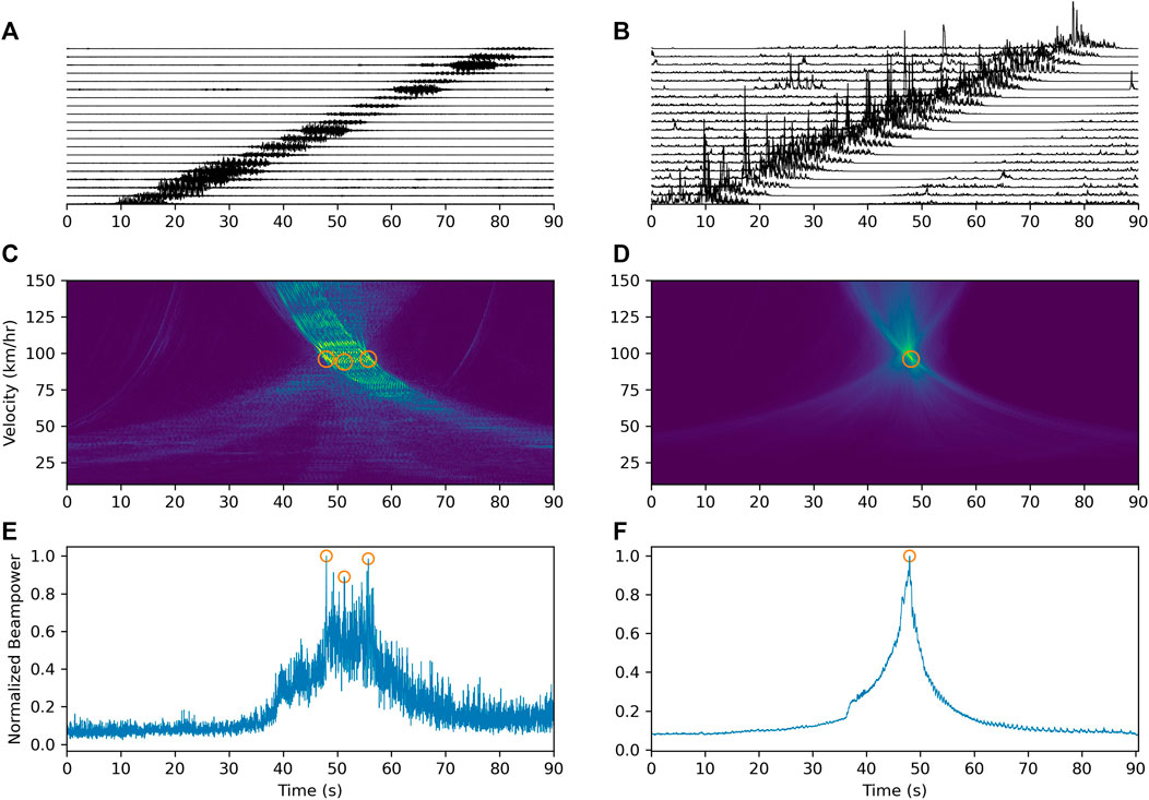
FIGURE 4. Comparison of beamforming results derived from raw signals and STA/LTA traces. (A) Signals extracted from the entire array every 50 channels; (B) STA/LTA traces of the signals shown in (A); (C) Vespagram calculated with the whole-array raw data; (D) Same as (C) but derived from STA/LTA traces; (E,F) Time-beampower curves of (C,D).

To avoid missed detection while processing long continuous data, we choose to select a small prominence parameter (usually could be 3 times the average of the noise amplitude). Similarly, to avoid false detection, we select a time-distance parameter that is larger than the signal duration of a slow train (set as 40 s). Figure 5 shows the detection and speed estimation results of the 1-h data earlier shown in Figure 2. From the observations, the train events are localized on the vespagrams and are successfully detected from the time-beampower curve. Also, we extract the speed after obtaining the corresponding local maximum beampower. In general, the higher the speed, the higher the beampower is and the better the automatic detection process performs. For the crossing and superimposed signals, our method also retrieves reliable results which demonstrates that our method can suitably be applied to heavy railway traffic monitoring.

FIGURE 5

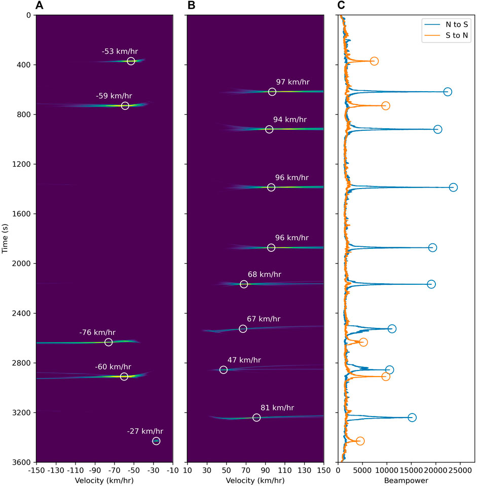
FIGURE 5. Beamforming results for a 1-h data (shown in Figure 2.). (A,B) Vespagrams for S-N and N-S trains and local power maximums detected from (C); (C) Time-beampower curve derived from (A,B), detected peaks denoted as circles.

Result

In Figure 6, we show the data detection result over a 6-day period, where it is observed that each detection time corresponds to the time the train passes the array center at Ch500. We qualitatively verify the detection results by visually inspecting the “footprints”, and categorize the types of trains by counting the number of peaks of the lowpass filtered waveforms (typical examples are shown in Figure 3). Due to the proprietary and sensitive nature of train itinerary records, we could not determine the exact train registration number of each passing/transiting train but constrained the type of trains by observing each passing train using their scheduled departure or arrival time (https://kyfw.12306.cn/otn/queryTrainInfo/init). From these records, we observe that the activity of railway traffic is somewhat irregular throughout the 6 days. Considering that the observation site is 5 km north of the railway station, the traffic pattern may not be an exact reflection of the exact time the train departed or arrived at the station. We also find out that some detected trains do not match the schedule, which could be either temporary or emergency scheduled trains or the trains that transits through the station without stopping. These scenarios are especially observed during between 23:00 to 7:00 (UTC+8), typical of the duration when non-scheduled trains operate. More so, we observe some signals with only one period which are believed to be generated by a single locomotive.

FIGURE 6

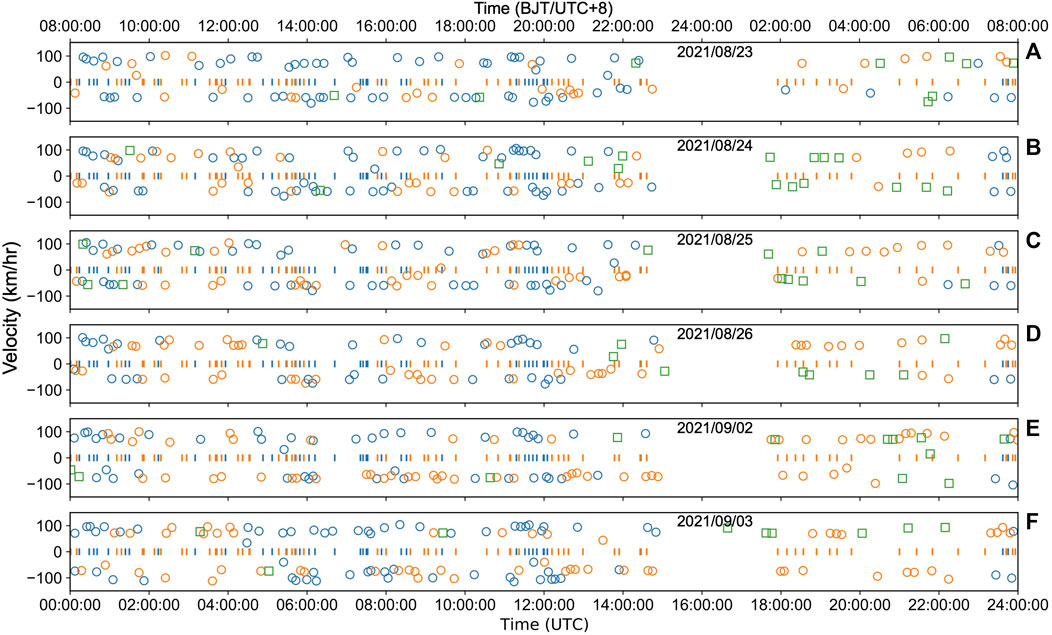
FIGURE 6. Detections, train speeds, and train types extracted from 6-days data. Negative and positive speed values correspond to N-S and S-N, respectively. Orange, blue vertical lines mark the time on the train timetable (the arrival time for N-S cases, and departure time for S-N). Orange and blue circles represent detected conventional trains and EMU trains, respectively; the hollow squares denote non-scheduled trains.

We count the detections based on the direction, speed, and type of trains (Figures 7A,B). Generally, we observe that the average speed of the trains from the north to the south is higher than those from the south to the north. This implies that at a distance of ∼5 km to the station, the deceleration time from the North to the South is shorter than the acceleration time from the South to the North. The speed is limited from block to block by the train control system (Ouyang et al., 2010; Zhang, 2008), which in practice, the train drivers adjust the speed while approaching or moving out of the train stations according to actual situations (CRC, 2004). Hence, there is no statistically significant difference in the speed of different types of trains in this case. The hourly detection histograms (Figures 7C,D) show similar railway traffic patterns on the both directions. The railway traffic becomes heavy during the morning and evening as similarly suggested in Figure 6, while turns out to be silent during the midnight.

FIGURE 7

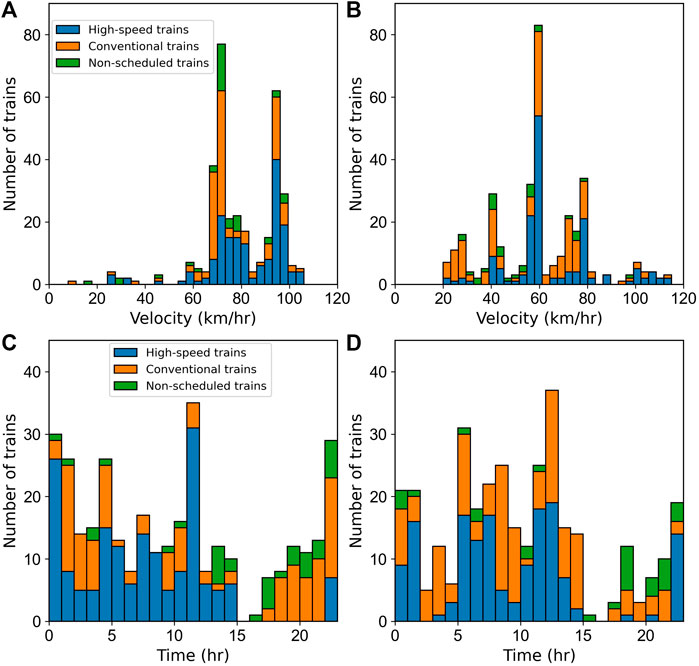
FIGURE 7. Histograms of speed distribution and hourly detections from N-S and S-N. (A,B) Speed distribution of all detected trains; (C,D) Hourly detections derived from the results shown in Figure 6.

Discussion

The cable is 2 km in length, as the cable cannot be perfectly straightened up, the real spatial distribution is theoretically shorter than the length of the cable. The estimated speed of our beamforming method is the apparent velocity along the cable, so we wish we could have the exact locations of each channel or some of them to correct this effect, however, we were not allowed to do it in the field work due to safety regulations of railways. Nevertheless, we observe that the trains pass our experimental site as constant speeds, which could be inferred from that the slope of the “footprints” is relatively constant. If the spatial distribution of the cable is complex, we could have seen twisted footprints and the beamforming results could be biased. From this point of view, we accept the shape of the cable causes minor effect in our study. In fact, the estimated speeds depend on the tolerance towards requirements if in real use, and we could correct the location of every channel by multiplying coefficients for the cable, thus we could exact more accurate speed of the trains passing our experimental site.

For an event generated by an individual train, an efficient way to evaluate its speed is to calculate the slope of the “footprint”, which implies, fitting linear regression on the arrival time of all the traces to verify the accuracy of the estimated speed retrieved through the beamforming method. Influenced by uneven coupling and possible orientation variations of the cable, simply utilizing STA/LTA algorithm across a dataset with equal threshold may not efficiently pick the arrival time. Considering the consistent duration of train-induced signals, we construct signal envelopes to reduce the complexity of waveforms (i.e., high-frequency noise, polarity reversals etc.), and calculate relative arrivals by conducting cross-correlation on Ch1 and the rest of the 1000 channels signal envelopes. We then apply the bootstrapping method (10,000 times) to quantify the variability of the linearly regressed velocities from the arrival times (Tichelaar and Ruff, 1989). To reduce the impact of the outliers on the regression calculation, we use the random sampling consensus algorithm (RANSAC; Fischler and Bolles, 1981; Yoo et al., 2020) to automatically exclude the outliers during each regression. Figure 8 shows the results from the linear regression of an EMU and a conventional train, respectively, as well as their bootstrapping histograms. The arrival times derived from the former have better convergence along with the signals than in the latter, thus indicating that the signals due to the EMU train are relatively more coherent. The outliers are identified and isolated by the RANSAC regressor (Figures 8B,E). The mean speed of the EMU and the conventional train are 96.18 and −25.69 km/h, respectively, whereas the standard deviations (STD) are 1.52 and 0.43 km/h, showing that the robust regression results are close to the beamforming estimations (96 and −26 km/h). Based on the STD of the speeds, the uncertainty of the EMU scenario is larger than that of the conventional train, which implies that the former has a larger speed variance. In general, the mean speeds of the two regression estimates are both within 1 km/h of the beamforming results, demonstrating that our method could achieve stable and accurate speed estimations with the DAS data.

FIGURE 8

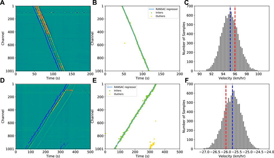
FIGURE 8. Examples of RANSAC linear regression on the relative travel times for EMU train and conventional train cases. (A) EMU train case and relative travel times (blue dots) picked by cross-correlation of signal envelopes; (B) RASAC regressor fitting the inliers, outliers excluded automatically; (C) Histogram of bootstrapped speeds, the red and blue dotted lines denote the beamformed speed obtained by our method and mean speed, respectively; (D–F) Same as (A–C), but for a conventional train case.

In actual situations, the length and coupling of the cable make the recorded DAS data impacted by different level of noise (Song et al., 2021). Therefore, we test the performance of our method on two typical train-event signals (Figure 8) with different noise levels. Before the start time of the signal window (40 and 50 s shown in Figures 8A,D; as zoomed in section in Figure9A,C), we slice the noise window into equal size with the signal window, and multiply the noise with factors ranging from 0 to 30. Thereafter, we impose the noise windows on the signal windows to obtain synthetic datasets with different noise levels and define the average signal-to-noise ratio (SNR) as the array energy (sum of the squared amplitude of all samples) ratio of the signal and noise windows (Lv et al., 2022). The initial SNR of the EMU and conventional train are 34.90 and 6.94 dB, respectively. As the SNRs decrease, the beampower values also decrease, and the false detections are not triggered until the SNRs fall as low as 0.81 dB for the EMU and 0.43 dB for the conventional train, corresponding to false peaks or multiple same-level peaks in the time-beampower curve (Figures 9B,D). In addition, we note that the least SNR required by the conventional train is less than that of the EMU, which could be due to its speed distribution that is assumed to be relatively more stable (Figures 8C,F).

FIGURE 9

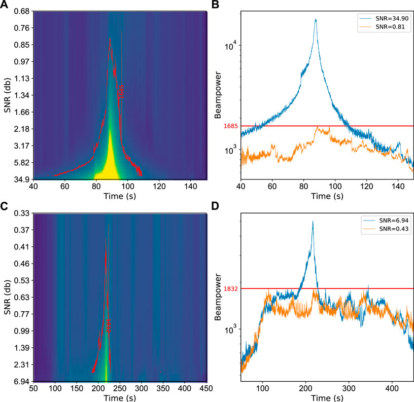
FIGURE 9. Examples of the beamforming performance influenced by different SNR levels. (A) Collection of time-beampower curves with different SNRs for an EMU train (sliced from the segment shown in Figure 8A), the red contour line marks the lowest beampower value leading to false detection. (B) Time-beampower curves under high SNR (blue line) and low SNR (red line), the latter leads to false detection. (C) Same as (A), but sliced from the segment shown in Figure 8D; (D) Same as (B), but extracted from (C).

For trains running at constant speed, the larger the array, the higher the beampower is and the more prominent the peak stands in the time-beampower curve. To ensure the reliability of results for actual railway traffic monitoring, using a smaller aperture will better enhance real-time monitoring. Moving small-aperture subarrays contribute to effectively monitor the change in speed of trains and update the track as the trains pass. However, smaller aperture will reduce the speed resolution on the vespagram (Nayak and Ajo-Franklin, 2021; Schweitzer et al., 2012). Moreover, the amplitude and duration of train-induced signals distinctively vary according to the type and speed of trains. Meanwhile, telecommunication cables suffer from coupling issues and varying noise levels or distributions (Song et al., 2021), so it is necessary to make adjustments on array aperture in compliance with real-time requirements and speed resolution. Figure 10 shows the beamforming results of an EMU train and a conventional train (same cases as shown in Figure 9) at different array apertures for the fiber-optic cable used in our experiment. We estimate the uncertainty by measuring 70% of the width of the detected peak amplitude in the time-beampower curve. With the increase of the array aperture, the results become more stable with less uncertainty (Figures 10B,E). To test the suitability of a certain aperture for the entire cable, we modify the aperture, move the array sequences every 50 channels, and beamform the data. Thus, we obtain detection results and velocity distributions as a function of array position along the cable (Figures 10C,F). For the EMU train, the speeds estimated from moving subarrays with a 60-channel aperture are sparser distribution than that of a 100-channel aperture. In the case of the conventional train, arrays with 150-channel aperture still lead to discrete speed estimations, while the 175-channel aperture produces more stable results. It is interesting to note that the edges of the train heads shown in Figure 10D are more identical than the rest wagons, which is often the case of low-speed conventional trains. We believe this is caused by the locomotive pulling the rest wagons. In practical or field situations, depending on the coupling and noise level, varying apertures can be used for different segments depending on the increase in the overlap of subarrays to obtain a denser velocity curve. Also, for seismological studies that utilize train-induced signals as noise sources, the real-time requirement is not urgent, in which case we could select a large array aperture.

FIGURE 10

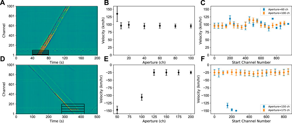
FIGURE 10. Array aperture test for an EMU train and conventional train. (A) EMU train case with different apertures/channels sliced as denoted by black squares; (B) Detection results with different apertures as shown in (A); (C) Detection results of moving arrays with 60 and 100-channel aperture; (D–F) Same as (A–C), but for a conventional train case.

Though most of the trains pass our experiment site at constant speeds, there are still individual cases where the speed changes significantly. Figure 11 shows the detection results of such a case with 150-channel moving subarrays from which the acceleration process of the train can be identified. From ∼ Ch1—Ch200, the time duration of signals covers ∼70 s. From–Ch200—Ch600, the duration decreases gradually to ∼20 s and thereafter remain constant till the end. We obtain the speed curve/motion track by smoothening the speed values, and the change in speed shown in the curve is consistent with the observation-based analysis shown above. Both 149 and 100-channel overlapping subarrays detect results with smooth and consistent velocity curves, which show that our methods also have good applicability in detecting trains moving at varying speed. In an extreme case, a high-speed train moving at a design speed of 350 km/h would take 3.09 s to cover a 150-channel array with 2 m channel spacing. In terms of computational efficiency, a NumPy 2D array npz file with a size of 1001 × 150000 (2 km and 300 s) can be loaded on an 8 G ram M1 chip MacBook Air within 0.2 s, and computation can be completed for a 150-channel aperture subarray matrix within 0.88 s. Such computational performance implies that our method is suitable for near real-time railway traffic monitoring. In addition, the Kalman filter is another approach to smooth the train trajectories (Ferguson et al., 2020; Wiesmeyr et al., 2020), and it would be interesting to test extended and adaptive Kalman filters (Terejanu, 2008; Vullings et al., 2010) on arrival picks and the detection results beamformed by subarrays. We could delve deeper into this in the future work.

FIGURE 11

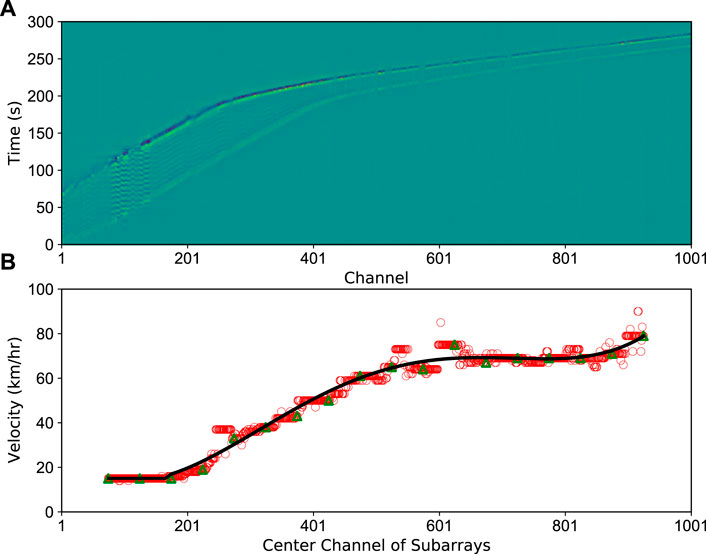
FIGURE 11. Speed and motion track estimation for a variable-speed train case. (A) Train-induced signals; (B) Detection results and speed distribution. Red circles denote the speed results estimated by moving subarrays with 149-channel overlapping, while green triangles denote the results with 100-channel overlapping. The black curve is the smoothed result of the green triangles.

Conclusion

In this study, we conduct an investigation on railway traffic monitoring using DAS data acquired by a 2-km trackside telecommunication fiber-optic cable. We utilize the beamforming technique on STA/LTA traces to automatically detect the train induced events, to extract their speed and direction. From the results, we identify the type of trains by counting the number of peaks from the lowpass filtered signal. Using beamforming technique, we process the 6-days continuous data to quantify and characterize the results using the speed, direction, and types of trains. By reducing the aperture of the array and moving subsequent subarrays, we obtain the train speed curve/motion track. The method we propose can provide a supplementary approach and play a synergetic role with other existing railway traffic monitoring systems. Moreover, our method can be used to conduct seismic interferometry investigation along the railroad using train-induced ground motions, whereby the noise windows containing or excluding train-induced signals can be automatically determined.

Data availability statement

The raw data supporting the conclusions of this article will be made available by the authors, without undue reservation.

Author contributions

GZ, ZS, and BC contributed to conception and design of the study. RL organized the database. AO revised English manuscript. GZ wrote the first draft of the manuscript. All authors contributed to manuscript revision, read, and approved the submitted version.

Funding

National Key R&D Program of China (2021YFA0716802), Knowledge Innovation Program of Wuhan‐Basic Research (S22H640301), National Natural Science Foundation of China (41974067).

Conflict of interest

The authors declare that the research was conducted in the absence of any commercial or financial relationships that could be construed as a potential conflict of interest.

Publisher’s note

All claims expressed in this article are solely those of the authors and do not necessarily represent those of their affiliated organizations, or those of the publisher, the editors and the reviewers. Any product that may be evaluated in this article, or claim that may be made by its manufacturer, is not guaranteed or endorsed by the publisher.

References

Ajo-Franklin, J. B., Dou, S., Lindsey, N. J., Monga, I., Tracy, C., Robertson, M., et al. (2019). Distributed acoustic sensing using dark fiber for near-sur- face characterization and broadband seismic event detection. Sci. Rep. 9, 1328. doi:10.1038/s41598-018-36675-8

PubMed Abstract | CrossRef Full Text | Google Scholar

Allen, R. (1978). Automatic earthquake recognition and timing from single traces. Bull. Seismol. Soc. Am. 68, 1521–1532. doi:10.1785/BSSA0680051521

CrossRef Full Text | Google Scholar

Baldini, G., Fovino, I. N., Masera, M., Luise, M., Pellegrini, V., Bagagli, E., et al. (2010). An early warning system for detecting GSM-R wireless interference in the high-speed railway infrastructure. Int. J. Crit. Infrastructure Prot. 3 (3-4), 140–156. doi:10.1016/j.ijcip.2010.10.003

CrossRef Full Text | Google Scholar

Brenguier, F., Boue, P., Ben-Zion, Y., Vernon, F., Johnson, C. W., Mordret, A., et al. (2019). Train traffic as a powerful noise source for monitoring active faults with seismic interferometry. Geophys. Res. Lett. 46 (16), 9529–9536. doi:10.1029/2019GL083438

PubMed Abstract | CrossRef Full Text | Google Scholar

Bruni, S., Goodall, R., Mei, T., and Tsunashima, H. (2007). Control and monitoring for railway vehicle dynamics. Veh. Syst. Dyn. 45 (7-8), 743–779. doi:10.1080/00423110701426690

CrossRef Full Text | Google Scholar

Cedilnik, G., Hunt, R., and Lees, G. (2018). “Advances in train and rail monitoring with DAS,” in 26th International Conference on Optical Fiber Sensors, Lausanne, Switzerland, September 24–28, 2018 (Optical Society of America). Paper ThE35. doi:10.1364/OFS.2018.ThE35

CrossRef Full Text | Google Scholar

Chambers, K. (2020). Using DAS to investigate traffic patterns at brady hot springs, Nevada, USA. Lead. Edge 39 (11), 819–827. doi:10.1190/tle39110819.1

CrossRef Full Text | Google Scholar

CRC (China Railway Corporation) (2004). Railway Technical Management Rules (normal speed railway section). Beijing: China Railway Press.

Google Scholar

Dou, S., Lindsey, N., Wagner, A. M., Daley, T. M., Freifeld, B., Robertson, M., et al. (2017). Distributed acoustic sensing for seismic monitoring of the near surface: A traffic-noise interferometry case study. Sci. Rep. 7 (1), 11620–11712. doi:10.1038/s41598-017-11986-4

PubMed Abstract | CrossRef Full Text | Google Scholar

Ferguson, R. J., McDonald, M. A. D., and Basto, D. J. (2020). Take the eh? train: Distributed acoustic sensing (DAS) of commuter trains in a Canadian city. J. Appl. Geophy. 183, 104201. doi:10.1016/j.jappgeo.2020.104201

CrossRef Full Text | Google Scholar

Fischler, M. A., and Bolles, R. C. (1981). Random sample consensus: A paradigm for model fitting with applications to image analysis and automated cartography. Commun. ACM 24 (6), 381–395. doi:10.1145/358669.358692

CrossRef Full Text | Google Scholar

Fuchs, F., and Bokelmann, G. (2017). Equidistant spectral lines in train vibrations. Seismol. Res. Lett. 89 (1), 56–66. doi:10.1785/0220170092

CrossRef Full Text | Google Scholar

Hudson, T. S., Baird, A. F., Kendall, J.-M., Kufner, S.-K., Brisbourne, A. M., Smith, A. M., et al. (2021). Distributed acoustic sensing (DAS) for natural microseismicity studies: A case study from Antarctica. JGR. Solid Earth 126 (7), e2020JB021493. doi:10.1029/2020JB021493

CrossRef Full Text | Google Scholar

Iswanto, I. A., and Li, B. (2017). Visual object tracking based on mean-shift and particle-Kalman filter. Procedia Comput. Sci. 116, 587–595. doi:10.1016/j.procs.2017.10.010

CrossRef Full Text | Google Scholar

Jiang, Y., Ning, J., Wen, J., and Shi, Y. (2022). Doppler effect in high-speed rail seismic wavefield and its application. Sci. China Earth Sci. 65 (3), 414–425. doi:10.1007/s11430-021-9843-0

CrossRef Full Text | Google Scholar

Kowarik, S., Hussels, M. T., Chruscicki, S., Munzenberger, S., Lammerhirt, A., Pohl, P., et al. (2020). Fiber optic train monitoring with distributed acoustic sensing: Conventional and neural network data analysis. Sensors (Basel). 20 (2), 450. doi:10.3390/s20020450

PubMed Abstract | CrossRef Full Text | Google Scholar

Lavoué, F., Coutant, O., Boué, P., Pinzon-Rincon, L., Brenguier, F., Brossier, R., et al. (2020). Understanding seismic waves generated by train traffic via modeling: Implications for seismic imaging and monitoring. Seismol. Res. Lett. 92 (1), 287–300. doi:10.1785/0220200133

CrossRef Full Text | Google Scholar

Li, Z., Shen, Z., Yang, Y., Williams, E., Wang, X., and Zhan, Z. (2021). Rapid response to the 2019 ridgecrest earthquake with distributed acoustic sensing. AGU Adv. 2 (2). doi:10.1029/2021av000395

CrossRef Full Text | Google Scholar

Lindsey, N. J., Martin, E. R., Dreger, D. S., Freifeld, B., Cole, S., James, S. R., et al. (2017). Fiber‐optic network observations of earthquake wavefields. Geophys. Res. Lett. 44 (23), 11–792. doi:10.1002/2017GL075722

CrossRef Full Text | Google Scholar

Lindsey, N. J., Yuan, S., Lellouch, A., Gualtieri, L., Lecocq, T., and Biondi, B. (2020). City-scale dark fiber DAS measurements of infrastructure use during the COVID-19 pandemic. Geophys. Res. Lett. 47 (16), e2020GL089931. doi:10.1029/2020GL089931

PubMed Abstract | CrossRef Full Text | Google Scholar

Liu, Y., Yue, Y., Luo, Y., and Li, Y. (2021). Effects of high-speed train traffic characteristics on seismic interferometry. Geophys. J. Int. 227 (1), 16–32. doi:10.1093/gji/ggab205

CrossRef Full Text | Google Scholar

Lv, H., Zeng, X., Bao, F., Xie, J., Lin, R., Song, Z., et al. (2022). ADE-net: A deep neural network for DAS earthquake detection trained with a limited number of positive samples. IEEE Trans. Geosci. Remote Sens. 60, 1–11. doi:10.1109/tgrs.2022.3143120

CrossRef Full Text | Google Scholar

Martin, E. R., Huot, F., Ma, Y., Cieplicki, R., Cole, S., Karrenbach, M., et al. (2018). A seismic shift in scalable acquisition demands new processing: Fiber-optic seismic signal retrieval in urban areas with unsupervised learning for coherent noise removal. IEEE Signal Process. Mag. 35 (2), 31–40. doi:10.1109/MSP.2017.2783381

CrossRef Full Text | Google Scholar

Meng, H., and Ben-Zion, Y. (2018). Detection of small earthquakes with dense array data: Example from the san jacinto fault zone, southern California. Geophys. J. Int. 212 (1), 442–457. doi:10.1093/gji/ggx404

CrossRef Full Text | Google Scholar

Nayak, A., and Ajo-Franklin, J. (2021). Distributed acoustic sensing using dark fiber for array detection of regional earthquakes. Seismol. Res. Lett. 92 (4), 2441–2452. doi:10.1785/0220200416

CrossRef Full Text | Google Scholar

Ouyang, M., Hong, L., Yu, M.-H., and Fei, Q. (2010). STAMP-based analysis on the railway accident and accident spreading: Taking the China–Jiaoji railway accident for example. Saf. Sci. 48 (5), 544–555. doi:10.1016/j.ssci.2010.01.002

CrossRef Full Text | Google Scholar

Parker, T., Shatalin, S., and Farhadiroushan, M. (2014). Distributed Acoustic Sensing–a new tool for seismic applications. First Break 32 (2). doi:10.3997/1365-2397.2013034

CrossRef Full Text | Google Scholar

Quiros, D. A., Brown, L. D., and Kim, D. (2016). Seismic interferometry of railroad induced ground motions: Body and surface wave imaging. Geophys. J. Int. 205 (1), 301–313. doi:10.1093/gji/ggw033

CrossRef Full Text | Google Scholar

Rost, S., and Thomas, C. (2002). Array seismology: Methods and applications. Rev. Geophys. 40 (3), 2-1–2-27227. doi:10.1029/2000rg000100

CrossRef Full Text | Google Scholar

Sager, K., Tsai, V. C., Sheng, Y., Brenguier, F., Boué, P., Mordret, A., et al. (2022). Modelling P waves in seismic noise correlations: Advancing fault monitoring using train traffic sources. Geophys. J. Int. 228 (3), 1556–1567. doi:10.1093/gji/ggab389

CrossRef Full Text | Google Scholar

Sasani, S., Asgari, J., and Amiri-Simkooei, A. R. (2015). Improving MEMS-IMU/GPS integrated systems for land vehicle navigation applications. GPS Solut. 20 (1), 89–100. doi:10.1007/s10291-015-0471-3

CrossRef Full Text | Google Scholar

Schweitzer, J., Fyen, J., Mykkeltveit, S., Gibbons, S. J., Pirli, M., Kühn, D., et al. (2012). Chapter 9 seismic arrays, in New manual of seismological observatory practice 2 (NMSOP-2). Dtsch. Geoforsch. GFZ, 22–25. doi:10.2312/GFZ.NMSOP-2

CrossRef Full Text | Google Scholar

Song, Z., Zeng, X., Xie, J., Bao, F., and Zhang, G. (2021). Sensing shallow structure and traffic noise with fiber-optic internet cables in an urban area. Surv. Geophys. 42, 1401–1423. doi:10.1007/s10712-021-09678-w

PubMed Abstract | CrossRef Full Text | Google Scholar

Spica, Z. J., Perton, M., Martin, E. R., Beroza, G. C., and Biondi, B. (2020). Urban seismic site characterization by fiber‐optic seismology. J. Geophys. Res. Solid Earth 125 (3), e2019JB018656. doi:10.1029/2019JB018656

CrossRef Full Text | Google Scholar

Tichelaar, B. W., and Ruff, L. J. (1989). How good are our best models? Jackknifing, bootstrapping, and earthquake depth. Eos Trans. AGU. 70 (20), 593–606. doi:10.1029/89EO00156

CrossRef Full Text | Google Scholar

Ulianov, C., Hyde, P., and Shaltout, R. (2018). Railway applications for monitoring and tracking systems. Sustainable Rail Transport. Cham: Springer, 77–91. doi:10.1007/978-3-319-58643-4_6

CrossRef Full Text | Google Scholar

van den Ende, M., and Ampuero, J. P. (2021). Evaluating seismic beamforming capabilities of distributed acoustic sensing arrays. Pacific Grove, CA: Solid earth 12 (4), 915–934. doi:10.5194/se-12-915-2021

CrossRef Full Text | Google Scholar

van den Ende, M., Ferrari, A., Sladen, A., and Richard, C. (2021). “Next-generation traffic monitoring with distributed acoustic sensing arrays and optimum array processing,” in 2021 55th Asilomar Conference on Signals, Systems, and Computers. doi:10.1109/IEEECONF53345.2021.9723373

CrossRef Full Text | Google Scholar

Virtanen, P., Gommers, R., Oliphant, T. E., Haberland, M., Reddy, T., Cournapeau, D., et al. (2020). Author correction: SciPy 1.0: Fundamental algorithms for scientific computing in Python. Nat. Methods 17 (3), 352–272. doi:10.1038/s41592-020-0772-5

PubMed Abstract | CrossRef Full Text | Google Scholar

Walter, F., Gräff, D., Lindner, F., Paitz, P., Köpfli, M., Chmiel, M., et al. (2020). Distributed acoustic sensing of microseismic sources and wave propagation in glaciated terrain. Nat. Commun. 11 (1), 2436–2510. doi:10.1038/s41467-020-15824-6

PubMed Abstract | CrossRef Full Text | Google Scholar

Wiesmeyr, C., Litzenberger, M., Waser, M., Papp, A., Garn, H., Neunteufel, G., et al. (2020). Real-time train tracking from distributed acoustic sensing data. Appl. Sci. (Basel). 10 (2), 448. doi:10.3390/app10020448

CrossRef Full Text | Google Scholar

Yoo, J., Mubarak, M. S., van Borselen, R., and Tsingas, C. (2020). “Line-guided first break picking via random sample consensus (RANSAC),” in SEG technical program expanded abstracts 2020 (Society of Exploration Geophysicists), 2044–2048. doi:10.1190/segam2020-3422645.1

CrossRef Full Text | Google Scholar

Yüksel, K., Kinet, D., Moeyaert, V., Kouroussis, G., and Caucheteur, C. (2018). Railway monitoring system using optical fiber grating accelerometers. Smart Mat. Struct. 27 (10), 105033. doi:10.1088/1361-665X/aadb62

CrossRef Full Text | Google Scholar

Zeng, X., Lancelle, C., Thurber, C., Fratta, D., Wang, H., Lord, N., et al. (2017). Properties of noise cross-correlation functions obtained from a distributed acoustic sensing array at Garner Valley, California. Bull. Seismol. Soc. Am. 107 (2), 603–610. doi:10.1785/0120160168

CrossRef Full Text | Google Scholar

Zhan, Z. (2019). Distributed acoustic sensing turns fiber‐optic cables into sensitive seismic antennas. Seismol. Res. Lett. 91 (1), 1–15. doi:10.1785/0220190112

CrossRef Full Text | Google Scholar